| Issue |
A&A
Volume 663, July 2022
|
|
|---|---|---|
| Article Number | A180 | |
| Number of page(s) | 10 | |
| Section | Stellar structure and evolution | |
| DOI | https://doi.org/10.1051/0004-6361/202243389 | |
| Published online | 28 July 2022 | |
Asteroseismology of evolved stars to constrain the internal transport of angular momentum
V. Efficiency of the transport on the red giant branch and in the red clump
1
Observatoire de Genève, Université de Genève, 51 Ch. Pegasi, 1290 Versoix, Suisse
e-mail: This email address is being protected from spambots. You need JavaScript enabled to view it.
2
Max Planck Institut für Sonnensystemforschung, Justus-von-Liebig-Weg 3, 37077 Göttingen, Germany
3
Instituto de Astrofísica e Ciências do Espaço, Universidade do Porto, CAUP, Rua das Estrelas, 4150-762 Porto, Portugal
4
LESIA, Observatoire de Paris, Université PSL, CNRS, Sorbonne Université, Université de Paris, 92195 Meudon, France
Received:
21
February
2022
Accepted:
4
May
2022
Abstract
Context. Asteroseismology provides constraints on the core rotation rate for hundreds of low- and intermediate-mass stars in evolved phases. Current physical processes tested in stellar evolution models cannot reproduce the evolution of these core rotation rates.
Aims. We investigate the efficiency of the internal angular momentum redistribution in red giants during the hydrogen-shell and core-helium burning phases based on the asteroseismic determinations of their core rotation rates.
Methods. We computed stellar evolution models with rotation and model the transport of angular momentum by the action of a sole dominant diffusive process parameterised by an additional viscosity in the equation of angular momentum transport. We constrained the values of this viscosity to match the mean core rotation rates of red giants and their behaviour with mass and evolution using asteroseismic indicators along the red giant branch and in the red clump.
Results. For red giants in the hydrogen-shell burning phase, the transport of angular momentum must be more efficient in more massive stars. The additional viscosity is found to vary by approximately two orders of magnitude in the mass range M ∼ 1–2.5 M⊙. As stars evolve along the red giant branch, the efficiency of the internal transport of angular momentum must increase for low-mass stars (M ≲ 2 M⊙) and remain approximately constant for slightly higher masses (2.0 M⊙ ≲ M ≲ 2.5 M⊙). In red clump stars, the additional viscosities must be an order of magnitude higher than in younger red giants of similar mass during the hydrogen-shell burning phase.
Conclusions. In combination with previous efforts, we obtain a clear picture of how the physical processes acting in stellar interiors should redistribute angular momentum from the end of the main sequence until the core-helium burning phase for low- and intermediate-mass stars to satisfy the asteroseismic constraints.
Key words: stars: rotation / stars: interiors / stars: evolution / methods: numerical
© F. D. Moyano et al. 2022
 Open Access article, published by EDP Sciences, under the terms of the Creative Commons Attribution License (https://creativecommons.org/licenses/by/4.0), which permits unrestricted use, distribution, and reproduction in any medium, provided the original work is properly cited.
This article is published in open access under the Subscribe-to-Open model. This email address is being protected from spambots. You need JavaScript enabled to view it. to support open access publication.
1. Introduction
The impact of rotation on the structure of stars and their evolution has been addressed since the early time of stellar physics (see e.g., von Zeipel 1924; Eddington 1929; Sweet 1950; Öpik 1951; Mestel et al. 1988). Grids of evolutionary rotating models have then been computed (see e.g., Endal & Sofia 1978; Pinsonneault et al. 1989; Deupree 1990; Fliegner et al. 1996; Heger et al. 2000; Meynet & Maeder 2000; Palacios et al. 2006; Ekström et al. 2012; Choi et al. 2017; Limongi & Chieffi 2018) based on the above first results and also based on more recent developments (e.g., Zahn 1992; Spruit 2002). Despite these long-term efforts, the transport of angular momentum (AM) in stellar interiors remains an open question. Our current picture of hydrodynamical transport of AM is insufficient to explain the rotation periods of compact objects (Suijs et al. 2008) and does not reproduce the internal angular velocity distribution deduced from helio- and asteroseismic analyses (see the discussion in Eggenberger et al. 2019c, and the next paragraph).
The long and continuous data sets obtained by space-borne missions, such as CoRoT (Baglin et al. 2009), Kepler (Borucki et al. 2010), TESS (Ricker et al. 2015), and in the future, PLATO (Rauer et al. 2014), led to the detection of mixed oscillation modes in evolved stars, which enabled to reveal their internal rotation. Interestingly, mixed oscillation modes are simultaneously sensitive to the physical properties in the central and external layers of a star. In particular, it was possible to gain information about the core rotation rates of subgiant and red giant stars at different evolutionary stages (Beck et al. 2012; Deheuvels et al. 2012, 2014, 2020, 2015; Mosser et al. 2012; Di Mauro et al. 2016, 2018; Triana et al. 2017; Gehan et al. 2018; Tayar et al. 2019). These data sets allow one to investigate in a statistical way the behaviour of AM redistribution in stellar interiors during their evolution in the subgiant and red giant phases. We know today that stellar models including only hydrodynamical processes fail to reproduce the angular velocity of stellar cores in different evolutionary phases (e.g., Eggenberger et al. 2012; Marques et al. 2013; Ceillier et al. 2013). In particular, the cores of stars on the lower red giant branch (RGB) rotate too fast by up to three orders of magnitude compared to expectations based on asteroseismic constraints. This indicates that at least one efficient additional AM transport process must be at work in the interior of evolved stars, similarly to what is found for the Sun (Eggenberger et al. 2005, 2019a) or for the rotation rates of compact objects (Suijs et al. 2008).
Several physical processes are candidates for this missing AM transport mechanism. Internal magnetic fields can transport AM efficiently in radiative regions and slow the stellar cores down. A first possibility relies on fossil magnetic fields to ensure uniform rotation in stellar radiative zones and on the assumption of radial differential rotation in the convective envelopes of evolved stars to account for the core rotation rates observed for these stars (Kissin & Thompson 2015; Takahashi & Langer 2021). This hypothesis is disfavoured by asteroseismic measurements of red giants, however, which are not compatible with a uniform rotation in the radiative interior of these stars (Klion & Quataert 2017; Fellay et al. 2021). Magnetic instabilities can also lead to an efficient AM transport in stellar radiative zones (Spruit 1999, 2002). Although they may be easily triggered above a certain degree of differential rotation, they are strongly inhibited by chemical gradients. Consequently, rotating models based on the Tayler-Spruit dynamo (Spruit 2002) are found to predict an internal coupling for red giants that is not efficient enough to reproduce their observed core rotation rates (Cantiello et al. 2014; den Hartogh et al. 2019). A revised formulation for this process leading to a more efficient AM transport than the Tayler-Spruit dynamo has then been proposed (Fuller et al. 2019). Lower core rotation rates are then obtained for evolved stars, which are in better global agreement with observed values, but asteroseismic measurements of subgiant, red giant, and secondary clump stars cannot be correctly reproduced (Eggenberger et al. 2019c; den Hartogh et al. 2020). Internal gravity waves may also transport AM in an efficient way. These waves can be excited by turbulent motions in convective zones (e.g., Press 1981), as well as by penetration of convective plumes (e.g., Pinçon et al. 2016, 2017). Gravity waves (especially those excited by penetrative convection) could play a role in shaping the rotation profile during the subgiant phase, but seem to be unable to influence the rotation in the central layers of red giant stars (Pinçon et al. 2017). Finally, AM transport by mixed oscillation modes could be a promising candidate for the upper part of the RGB (Belkacem et al. 2015). We highlight, however, that neither internal gravity waves nor mixed modes can extract AM efficiently from the cores of stars close to the RGB base, where they might spin up considerably. The physical process responsible for the AM transport in this rapid phase is still unknown.
We thus see that we are still far from having a physical explanation to the internal rotation observed in evolved stars. It is then valuable to use asteroseismic measurements to characterise at best the properties of this unknown transport process to try to reveal its physical nature.
We do this in a similar way as in previous works (see Eggenberger et al. 2012, 2019b, 2017; Spada et al. 2016; den Hartogh et al. 2019), although in this paper we focus solely on the evolution of the core rotation rate and take advantage of a larger number of stars with well-characterised asteroseismic properties (see Sect. 2.3). This in turn allows us to draw conclusions about the role of the stellar mass and evolution along the red giant phase. We also compute low-mass stellar models in the core-helium burning phase, hence complementing the efforts done for the more massive secondary-clump stars (e.g., Tayar & Pinsonneault 2013, 2018; Tayar et al. 2019; den Hartogh et al. 2019). We parametrise the efficiency of the unknown transport process by a constant additional viscosity (νadd) in the equation of AM transport. We do not expect the undetermined AM transport process(es) to be effectively described by this simple assumption of a constant viscosity in stellar radiative zones, but this approach enables us to quantify the efficiency with which they must operate to satisfy the empirical constraints. More precisely, it enables us to probe how the efficiency of this additional transport process has to vary with mass and time in different evolutionary phases. This can place constraints on the nature of the physical processes acting in stable stratified regions. The mean viscosities derived in this work may also serve as benchmark values for ongoing theoretical developments and numerical multi-dimensional simulations, for instance the AM transport by the azimuthal magnetorotational instability (AMRI; Rüdiger et al. 2014) or by the Goldreich-Schubert-Fricke instability (GSF; Barker et al. 2019, 2020).
Asteroseismic constraints indicate that in subgiants, the AM redistribution must occur very efficiently just after the main sequence (MS) and then gradually weaken towards the RGB (Eggenberger et al. 2019a; Deheuvels et al. 2020). AM redistribution has also been found to be more efficient as stars ascend the RGB with an efficiency that increases with stellar mass (Eggenberger et al. 2017). The change in efficiency with evolution between the subgiant and the red giant phase might indicate that different physical processes act in these two phases, or if the processes are the same, to significantly different consequences due to different physical conditions in stellar interiors. For instance, the timescale for the crossing of the Hertzsprung gap and the ascent of the RGB are governed by different processes. While this crossing is linked to the contraction of the core and the expansion of the envelope on a rapid timescale, the ascent of the RGB occurs on a longer nuclear timescale. In this last case, the evolution is due to the growing helium core resulting from the activity of the H-burning shell. The transition between these two phases is thus a key point to understand.
The previously mentioned study of Eggenberger et al. (2017) was based on two well-characterised targets so that a confirmation of these trends with larger samples is still lacking. Here we aim to fill this gap using a sample of hundreds of red giants obtained by Gehan et al. (2018) with determined rotational splittings of dipole mixed modes and asteroseismic quantities. This enables us to better characterise their evolutionary stage. We finally complement our study with data of red clump stars using the sample of Mosser et al. (2012).
In Sect. 2 we describe the tools we used and the input physics of the stellar models. In Sect. 3 we present the models we computed and the additional viscosities we inferred to discuss their implications and global behaviour during the evolution in Sect. 4. We summarise our main results in Sect. 5.
2. Stellar models and data
2.1. Input physics: Red giants
We computed stellar evolution models of red giants, starting from the zero-age main sequence (ZAMS), with the Geneva stellar evolution code (qcrGENEC; Eggenberger et al. 2008). We refer to the mentioned work for details on the input physics and numerical treatment. We briefly explain the most relevant parameters we used to compute the models presented in this work, and in particular for the modelling of AM transport in stellar interiors. Rotation is treated assuming shellular rotation (Zahn 1992). The equation to follow the evolution of the AM is treated in an advecto-diffusive way (see Eq. (1)). In convective zones we assumed solid-body rotation. For radiative zones, the equation
 (1)
(1)
is solved, where r and ρ stand for radius and mean density on an isobar, Ω is the horizontally averaged angular velocity, U(r) expresses the radial dependence of the vertical component of the meridional circulation velocity, and D is the diffusion coefficient. The diffusive term of this equation (second on the right side) is responsible for decreasing the differential rotation in radiative regions as it acts on the shear, denoted here by ∂Ω/∂r. The diffusion coefficient D takes the diffusive processes as a linear sum of each of them into account. For the diffusion of AM, we include the shear instability (Dshear; Maeder 1997) and a constant additional viscosity (νadd), hence D = Dshear + νadd.
In all of our models we adopt solar metallicity with the solar chemical mixture given by Asplund et al. (2009). We also use a value calibrated on the Sun for the mixing-length parameter. The remaining physical ingredients, such as overshooting and mass loss, are the same as in Ekström et al. (2012).
2.2. Input physics: Core-helium burning stars
To explore the transition towards the core-helium burning phase of low-mass stars, we used the qcrMESA stellar evolution code (Paxton et al. 2011, 2013, 2015, 2019), version 151401. The use of the qcrMESA code enables us to study the internal rotation of red clump stars (low-mass stars in the core-helium burning phase), since the qcrGENEC code does not routinely follow the rotational evolution of stars after the helium flash. Moreover, using two evolutionary codes with different implementations of rotational effects enables us to verify that the results obtained about the AM transport efficiency in stars ascending the RGB are not too sensitive to the specific code that is used.
Rotation in qcrMESA was treated following Heger et al. (2000), and we refer to that work for further details. Although the treatment of rotation in qcrMESA is purely diffusive, while it is an advecto-diffusive process as treated in qcrGENEC, we verified that the results and conclusions derived in this work are independent of the code used. This is due to the fact that AM transport by meridional currents and the shear instability is negligible in the type of evolved stars that we study in this work. The equation used in qcrMESA to follow the evolution of the AM transport is
![Mathematical equation: $$ \begin{aligned} \left( \frac{\partial \Omega }{\partial t}\right)_m=\frac{1}{j}\left( \frac{\partial }{\partial m}\right)_t \!\left[ (4\pi r^2 \rho )^2jD \left( \frac{\partial \Omega }{\partial m}\right) \right]-\frac{2\Omega }{r}\!\left(\frac{\partial r}{\partial t}\right)_m\left( \frac{1}{2}\frac{\mathrm{d ln}\,j}{\mathrm{d ln}\,r}\right) , \end{aligned} $$](/articles/aa/full_html/2022/07/aa43389-22/aa43389-22-eq2.gif) (2)
(2)
where j is the specific angular momentum. The remaining variables are defined as in Eq. (1). The additional viscosity νadd is added linearly in the diffusion coefficient D in the first term. For consistency with our qcrGENEC models, we only account for transport of AM by the shear instability and meridional circulation (in addition to νadd) in radiative regions.
2.3. Asteroseismic constraints
To study the redistribution of AM at different evolutionary phases and for different mass ranges, we compiled a data set with constraints on the core rotation rate for low- and intermediate-mass stars. The core and surface rotation rate of eight subgiants was obtained by Deheuvels et al. (2014, 2020). Gehan et al. (2018) obtained the rotational splittings of 875 stars in the RGB in a systematic way. The mass of these stars, as estimated by asteroseismic scaling relations (e.g., Kallinger et al. 2010), is in the range M ∼ 1–2.5 M⊙.
We also benefit from the asteroseismic quantities derived in the mentioned work, namely the large frequency separation (Δν), the period spacing (ΔΠ1), and the frequency of the maximum oscillation signal (νmax). We used the rotational splittings of the most strongly g-dominated modes, as given by Gehan et al. (2018), to estimate the core rotation rate of all stars in the sample. This can be done under the assumption that gravity-dominated dipole mixed modes are mainly sensitive to the core. However, the rotational splittings in the lower part of the RGB (before the bump) could be affected by the envelope. To account for this contamination, a correction factor can be introduced with the help of the asteroseismic quantities mentioned above (Mosser et al. 2012). In this way, the mean core rotation rate can be obtained from the rotational splittings as (Goupil et al. 2013)
 (3)
(3)
where δνrot, core is the measured core rotational splitting, and η is the correction factor mentioned above. This correction factor can be computed as
 (4)
(4)
where γ ≃ 0.65 (Mosser et al. 2012) and 𝒩 is the mixed-mode density (see Eq. (5) below). This correction factor η is slightly larger than unity for stars close to the RGB base and decreases towards unity as they ascend it. Using this correction factor decreases the margin of error on the mean core rotation rate obtained from g-dominated mixed modes instead of pure gravity ones. Quantifying the difference in the retrieved mean core rotation rate when using g-dominated mixed modes instead of pure gravity modes would require the use of rotational kernels derived from stellar structure models and the assumption of a rotation profile. This is beyond the scope of this work. Nevertheless, the envelope contribution to the splitting of g-dominated modes is negligible (Mosser et al. 2012), hence we do not expect important differences. Additionally, the uncertainties from Gehan et al. (2018) on the measured rotational splittings can be translated into uncertainties on the estimated core rotation rate. However, they are ∼10 nHz, which leads to a maximum uncertainty of ∼30 nHz on the mean core rotation rate for our hydrogen-shell burning stars. Thus, for clarity, we decided not to include the associated error bars in any of our figures since in many cases, they would be even smaller than the symbol size.
The resulting distribution of core rotation rates for different mass ranges is shown in Fig. 1. We do not intend to re-analyse the distribution seen for these stars because this was reported by Gehan et al. (2018). Nevertheless, it is worth recalling that most of these stars have core rotation rates in the range ⟨Ωcore⟩/2π ∈ [600, 800] nHz, a mean mass of ∼1.5 M⊙, and their core rotation rates do not show any dependence on mass or evolution (see Figs. 10 and 11 from Gehan et al. 2018).
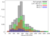 |
Fig. 1. Fraction of stars as a function of the mean core rotation rate for the full sample of hydrogen-shell burning stars from Gehan et al. (2018), and for different stellar mass ranges as indicated in the figure in units of solar masses. |
As suggested by Gehan et al. (2018), we used the mixed-mode density (𝒩) as a proxy for the specific evolutionary phase along the RGB. This physical quantity is equal to the number of gravity modes within a frequency range whose width is equal to the large frequency separation. It is defined as
 (5)
(5)
To compare it with our model results, we computed the asymptotic large frequency separation. The νmax frequency was obtained using global asteroseismic scaling relations (see e.g., Kjeldsen & Bedding 1995; Kallinger et al. 2010). We computed the asymptotic estimate of the period spacing from the structure of each model as
 (6)
(6)
where NBV is the Brunt-Väisälä frequency, and r is the radial coordinate. The integral was done over the g-mode cavity, with rg the radius of the upper limit of the cavity.
The core rotation rate inferred with asteroseismic techniques is an average value of the angular velocity near the core, because it is related to the regions tested by gravity modes; it is not the angular velocity of the centre. Hence, to compare directly our results with the constraints available from asteroseismic techniques, we computed the mean core rotation rate ⟨Ωcore⟩ from our models as (Goupil et al. 2013)
 (7)
(7)
where Ω is the angular velocity, and r is the radial coordinate. This integral is computed over the g-mode cavity, and represents the angular velocity in the near-core region as sensed by gravity modes.
Finally, for low-mass stars in the core-helium burning phase, we used the constraints on the mean core rotation rate given by Mosser et al. (2012). In this case, we only used the mean core rotation rate, and we used the mass and radius estimated via scaling relations. We did not use the mixed-mode density as an evolution indicator for core-helium burning stars in this work.
3. Efficiency of the angular momentum redistribution
In this section we present the results for the efficiency needed for the AM transport to satisfy the asteroseismic constraints presented in Sect. 2.3. We first present the role of the stellar mass on the efficiency of the angular momentum redistribution for red giants in the hydrogen-shell burning phase (Sect. 3.1). Then we show how this efficiency should vary with evolution along the lower RGB (Sect. 3.2). We finally present a similar analysis for low-mass (M ≲ 2 M⊙) core-helium burning stars (Sect. 3.3).
3.1. Mass dependence of red giants
To investigate the mass dependence of the additional viscosity needed to satisfy the asteroseismic constraints, we computed a grid of models with different initial masses and additional viscosities. We computed models in the mass range of 1.1–2.5 M⊙, which covers the whole mass range in the data set presented in Sect. 2.3, according to the scaling relations. In this series of models, we started the models from the ZAMS and adopted an initial period of P = 10 days (see Sect. 4.1 for a discussion of the impact of this choice). We chose this initial period since it roughly reproduces the surface rotation rates of subgiants, for which a detailed asterosesimic characterisation of their internal rotation was obtained by Deheuvels et al. (2014). For each model with a different initial mass, we adopted a range of values for νadd suitable to reproduce the bulk of the data. To refine the estimates on νadd for each mass value, we ultimately interpolated between tracks with the same initial mass and different νadd when the difference in νadd between adjacent models was small enough, typically smaller than 10%.
In Fig. 2 we show a subset of our models with a constant additional viscosity of νadd = 8 × 103 cm2 s−1 and the data set of red giants in the hydrogen-shell burning phase from Gehan et al. (2018). We chose this value of νadd because it can reproduce the core rotation rate of most of the red giants for a stellar model with an initial mass of M = 1.1 M⊙. The curves show the evolution of the mean core rotation rate for different initial masses, starting from the ZAMS and ending just above the RGB bump. This is seen at log g ∼ 2.5 for stars with a mass lower than M ∼ 2 M⊙. This figure illustrates two important points of this study: (i) the majority of stars are grouped in a narrow band with ⟨Ωcore/2π⟩ = 700 ± 100 nHz and surface gravity in the range log g ∼ 2.9–3.3 (we refer to this band as the bulk of the data), and (ii) to correctly reproduce the bulk of the data, AM redistribution needs to increase its efficiency as mass increases in red giants close to the base of the RGB.
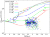 |
Fig. 2. Evolution of the core rotation rate as a function of the surface gravity. The data points correspond to the red giants in the hydrogen-shell burning phase analysed by Gehan et al. (2018) and are colour-coded by their mass as for the models. Each model has a different initial mass, as indicated in the figure. An additional viscosity of νadd = 8 × 103 cm2 s−1 was used in all models. |
To obtain a quantitative estimate of how the value of νadd varies with mass as well as an estimate of its uncertainty, we determined the value needed for each model in order to obtain a core rotation rate of ⟨Ωcore⟩/2π = 700 ± 100 nHz at a surface gravity of log g = 3.1 ± 0.2 dex. For low-mass stars, the interval we used in surface gravity represents the largest source of error in our estimates of νadd. In our models, the core rotation rate increases significantly during the evolution (see e.g., the red line in Fig. 3). This behaviour requires the use of different νadd values during the evolution to achieve a core rotation rate of ⟨Ωcore⟩/2π ∼ 700 nHz, which was then used to estimate the uncertainty on νadd for each given stellar mass. On the other hand, the interval used in core rotation rate only results in a small uncertainty on νadd for low-mass stars. The situation is reversed for intermediate-mass stars (M ≳ 2 M⊙). In this case, the core rotation rate obtained in our models does not vary much during the evolution in the region in which measurements are available (see e.g., the cyan line in Fig. 3). As a consequence, we can maintain a rate of ⟨Ωcore⟩/2π ∼ 700 nHz with a roughly constant value of νadd along evolution on the lower RGB. The source of uncertainty thus here mainly comes from the interval used in core rotation rate. However, the evolution of the core rotation rate is very sensitive to the adopted νadd value, so that small variations in νadd result in significantly different core rotation rates. The possible range of νadd values that allows matching the available measurements for intermediate-mass stars is therefore small. This results in smaller uncertainties in νadd for intermediate-mass stars compared to low-mass stars.
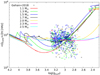 |
Fig. 3. Same as Fig. 2, but for models with the additional viscosity νadd that is needed to match the mean core rotation rate of red giants in the hydrogen-shell burning phase. The values of the additional viscosities for each model used in this figure are shown in Fig. 5 and given in Table 1. |
The resulting models with the values of νadd that we found are shown in Fig. 3. In this figure, the core rotation rates of the low-mass models (M ≲ 2 M⊙) behave in a similar way when they start climbing the RGB (for log g ≲ 3.5). This occurs because the relative change in the core rotation rate ( ) of low-mass stars converges to roughly the same value towards the RGB (see Fig. 4). The first narrow peak located for example at log g ∼ 4 for the 1.5 M⊙ model in Fig. 4 occurs at the end of the main sequence and is a consequence of the rapid contraction in which the surface radius decreases and leads to the hook-like feature seen in the HR diagram. The second broader peak, occurring around log g ∼ 3.6 − 3.7 for the 1.5 M⊙ model in Fig. 4, is a second contraction of the central layers that occurs halfway through the subgiant phase (Eggenberger et al. 2019b). Since the additional viscosity sets the conditions for these models to have the same core rotation rate close to the base of the RGB, the increase in their core rotation rate shown in Fig. 3 is similar, leading to almost overlapping core rotation rates. This is different for the more massive models, with masses higher than M ≳ 2 M⊙ (see Fig. 3), which have an increasing relative contraction rate
  (or decreasing contraction timescale) with mass (see Fig. 4).
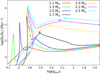 |
Fig. 4. Contraction rate of the core as a function of the surface gravity for models without additional viscosity. Stars with masses lower than M ≲ 2 M⊙ converge towards the same contraction rate at low surface gravity. |
The additional viscosity required to match the core rotation rate of the red giants is shown in Fig. 5 as a function of the initial mass. We list the estimated values of νadd in Table 1. We performed the analysis using both the surface gravity and the mixed-mode density (𝒩) separately, and we found consistent results. To estimate the uncertainty (error bars) in the estimates of νadd given in Table 1, we considered the values of νadd that can reproduce a core rotation rate of ⟨Ωcore/2π⟩ = 700 nHz at log g = 3.1, allowing for an uncertainty of 100 nHz and 0.2 dex in core rotation rate and surface gravity.
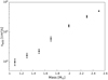 |
Fig. 5. Dependence of the additional viscosity (proxy for the efficiency of angular momentum redistribution) on the stellar mass in red giants in the hydrogen-shell burning phase. These values are estimated at a surface gravity of log g ∼ 3.1, or equivalently, at a mixed-mode density of 𝒩 ∼ 7. Including these values in stellar evolution models leads to core rotation rates that agree with asteroseismic constraints. The values are given in Table 1. |
3.2. Dependence on the evolution along the red giant branch
To investigate if there is any dependence on the evolution along the RGB, we resorted to the mixed-mode density (𝒩). As shown by Gehan et al. (2018), this quantity is an interesting proxy for the evolutionary stage of a star on the RGB because it is mainly sensitive to the size of the helium core in the red giant phase. We followed the same approach as in Sect. 3.1 to study the dependence of νadd on the evolution. The evolution of the core rotation rate as a function of the mixed-mode density for different initial masses is shown in Fig. 6 for a subset of models with a constant additional viscosity of νadd = 8 × 103 cm2 s−1. The corresponding models with the calibrated additional viscosities are shown in Fig. 7. To quantify the evolution along the RGB based on the mixed-mode density, we chose three representative values of the data bulk, at 𝒩 = 4, 9, and 14.
We illustrate this in Fig. 8 for a 1.5 M⊙ model in which we show the effect of changing the additional viscosity to match the core rotation rate at the three different locations chosen in the data set. We show the values of νadd during the evolution on the RGB in Fig. 9 for different initial masses. In this figure, νadd is normalised to the value required to match the data bulk at 𝒩 = 4 to disentangle the change during the evolution from the mass dependence (see Fig. 5).
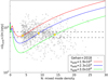 |
Fig. 8. Core rotation rate as a function of the mixed-mode density for models during the hydrogen-shell burning phase. The efficiency of AM redistribution (parametrised by the additional viscosity νadd) varies in order to reproduce the mean evolution of the core rotation rate as given by asteroseismic constraints for a 1.5 M⊙ model with an initial period of Pini = 10 days at three different locations (𝒩 = 4, 9, and 14), shown with yellow dots on the evolutionary tracks. The dotted lines show the interval in which ⟨Ωcore⟩/2π ∈ [600, 800] nHz. |
For low-mass stars, the additional viscosity can increase up to a factor of two in the lower part of the RGB, while for stars with an initial mass of M ≳ 2 M⊙, the additional viscosity remains roughly constant (Fig. 9). Moreover, the variation of the additional viscosity along evolution tends to become weaker as the mass increases. The normalised νadd values are lower as the mass increases for each of the three 𝒩 values we considered, and νadd even decreases slightly for the highest mass stars in our sample.
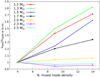 |
Fig. 9. Additional viscosity needed to satisfy the rotational constraints of red giants in the hydrogen-shell burning phase, normalised to its value at a mixed-mode density of 𝒩 = 4, as a function of the mixed-mode density. The different curves correspond to different initial masses, as indicated in the legend. |
3.3. Low-mass core-helium burning stars
To study the efficiency of AM transport in red clump stars, we computed models until the end of the core-helium burning phase with initial masses of M = 1–2 M⊙ using different additional viscosities, as outlined in Sect. 3.1. The evolution of the core rotation rate as a function of the radius is shown in Figs. 10 and 11. In these figures, we show the data of Mosser et al. (2012) for stars with a mass of M ≲ 2 M⊙, to avoid including secondary clump stars that are intermediate-mass stars (2 ≲ M/M⊙ ≲ 8) in the core-helium burning phase (e.g., Girardi et al. 1998). We verified that the additional viscosity must increase from the red giant phase towards the core-helium burning phase. This is because the additional viscosity calibrated for red giants is not sufficient for the red clump stars. This is shown by the model with νadd = 1.5 × 104 cm2 s−1 in Fig. 10, which can match the rotation rate of red giants, but not that of core-helium burning stars. Considering the bounds on the core rotation rates from the data sets, we find that an additional viscosity of νadd = (3 ± 2)×105 cm2 s−1 is suitable to reproduce the core rotation rate of the red clump stars (see Fig. 10). This value does not depend on the initial mass.
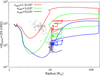 |
Fig. 10. Evolution of the core rotation rate as a function of the stellar radius. All models have an initial mass of 1.2 M⊙ and an initial velocity of 5 km s−1 (Pini = 12 days) and were computed with qcrMESA. Different values for the additional viscosity are used in each model, as indicated in the figure in units of cm2 s−1. The sharp drop in core rotation rate seen at R ∼ 150 R⊙ occurs because of the helium flash. The data correspond to red giants and red clump stars from Mosser et al. (2012). Only stars (data) with an estimated mass lower than M ≲ 2 M⊙ were included. Red clump stars are grouped at radii R ∼ 10 R⊙ (crosses), and red giants in the hydrogen-shell burning phase are located above this, with a higher core rotation rate and lower radii (circles). |
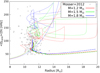 |
Fig. 11. Same as Fig. 10, but for models with different initial masses, as indicated in the legend. We show only the region around the stable core-helium burning phase. All models have an additional viscosity of νadd = 5 × 105 cm2 s−1. The data points correspond to red clump stars from Mosser et al. (2012). Dotted lines: before stable core-helium burning. Solid lines: long and stable core-helium burning phase (see text). Dash-dotted lines: last fraction of the stable core-helium burning phase. |
The core slows down most strongly during the first He-flash, when the degeneracy is lifted and the core expands. In this short phase, the core angular velocity decreases by ∼70%. This causes the sharp drop in Fig. 10 in the core rotation rate at a constant stellar radius of R ∼ 150 R⊙. The relative decrease at constant radius in core rotation rate is independent of both the viscosity adopted and the initial mass, although the exact angular velocity of the core at the RGB tip depends on these two parameters. This phase is so short that the adopted value of the viscosity at the RGB tip does not make any difference in the subsequent evolution. The loops seen after the drop in ⟨Ωcore⟩ after the star contracts are secondary flashes and last less than ∼4 Myr in total. Afterwards, the models enter the stable core-helium burning phase (when the mass fraction of central helium drops below ∼0.9) and spend more than ∼85 % of their burning time with a roughly constant radius of R ∼ 10–11 R⊙. This corresponds to ∼100 Myr.
The models with an additional viscosity of νadd ∼ 105 cm2 s−1 spend most of their core-helium burning time with a core rotation rate that agrees with the upper end of the data bulk for red clump stars, which corresponds to ⟨Ωcore/2π⟩∼150 nHz (see Fig. 10). Before this phase, they are in a short phase, and thus we adopt νadd ∼ 105 cm2 s−1 as a lower limit for the additional vicosity. On the other hand, models with initial viscosities above νadd ∼ 5 × 105 cm2 s−1 spend most of the time during the stable core-helium burning phase at lower core rotation rates than those of the data bulk (i.e. ⟨Ωcore/2π⟩≲50 nHz). Because of this, we constrained the upper value of the additional viscosity to νadd ∼ 5 × 105 cm2 s−1. Therefore, an acceptable value of the additional viscosity for red clump stars is νadd = (3 ± 2)×105 cm2 s−1. This value is weakly dependent on the stellar mass. We illustrate this in Fig. 11 for models with different initial masses. The dotted lines show the region before the stable helium burning phase, solid lines show the region in which the model spends ∼85% of the duration in the core-helium burning phase, and in the regions of the dot-dashed lines, it spends the remaining time until the end of the core-helium burning phase. This behaviour does not depend on the initial mass. We therefore find that the inferred additional viscosity is weakly dependent on the stellar mass in this evolutionary phase. We note that it is difficult to reproduce the observed spread in radii in the red clump with our models. This might be accounted for with a distribution of initial metallicities because we recall that in all our models, we adopted a solar chemical composition.
4. Global behaviour of the AM redistribution
In the previous section, the efficiency of AM redistribution was determined for red giants in the hydrogen-shell and core-helium burning phases. Now we compare our results to those obtained in previous works for subgiants and secondary clump stars. In line with our work, the additional viscosity needed to satisfy the constraints on eight subgiants has been obtained in previous works (Eggenberger et al. 2019b; Deheuvels et al. 2020). For two of these subgiants located close to the end of the main sequence, asteroseismic data are consistent with the fact that they are rotating as solid bodies. Because of this, Deheuvels et al. (2020) could only estimate a lower boundary on the additional viscosity, high enough to ensure the compatibility with asteroseismic constraints on core and surface rotation rates.
In Fig. 12 we show the change in νadd with the evolution that we obtained for red giants compared to those inferred for subgiants. Following Eggenberger et al. (2019b), we used the radius of the star normalised to its radius at the end of the main sequence as a proxy for the evolution. We note that the average mass of the subgiants is M ∼ 1.2 M⊙ and that the highest-mass star has an inferred mass of M = 1.4 M⊙. Since there is a mass-dependence for the red giants that we studied, we show the evolution of νadd for different masses. It was already shown that the higher the stellar mass of subgiants, the more efficient the redistribution of AM (Eggenberger et al. 2019a). It also seems to be very efficient just after the main sequence, as inferred from the two young subgiants studied by Deheuvels et al. (2020). Later in the subgiant phase, its efficiency decreases until it reaches a minimum value close to the base of the RGB, to progressively increase afterwards as the star becomes a larger red giant.
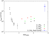 |
Fig. 12. Evolution of the efficiency of AM redistribution, parametrised by the additional viscosity νadd, as a function of the radius normalised to the radius at the end of the MS. Black dots with R/RTAMS < 2 correspond to subgiants studied by Deheuvels et al. (2020) and Eggenberger et al. (2019b). The other symbols correspond to red giants in the phase of hydrogen-shell burning with different initial masses and finally to the estimate for red clump stars based on a 1.2 M⊙ model. |
We showed in Sect. 3.3 for red clump stars that an additional viscosity of νadd = (3 ± 2)×105 cm2 s−1 is needed to reproduce their core rotation rate. The horizontal error bars shown in Fig. 12 come from the spread in radius of the data set. The fact that the efficiency needed to reproduce the core rotation rate of red giants is not enough for red clump stars suggests that the efficiency must increase during the evolution on the RGB and must couple the core more strongly with the envelope. We do see this trend with evolution at least on the lower RGB (see Fig. 12). However, for red-clump stars we found an additional viscosity lower than what was obtained for secondary-clump stars by den Hartogh et al. (2019). They found that the additional viscosity must have a value of νadd = 107 cm2 s−1, which is almost two orders of magnitude higher than for red-clump stars. Since our sample comprises only stars with a mass of M ≲ 2 M⊙, the higher value for secondary clump stars might indicate a dependence on mass in the core-helium burning phase as well, or an indirect impact due to the structural and evolutionary differences between stars that burn helium in their core in a non-degenerate way (M ≳ 2 M⊙) compared to those that do not, and thus go through the helium flash phase (M ≲ 2 M⊙).
4.1. Sensitivity to initial assumptions
In our series of models we estimated the additional viscosity for red giants by adopting the same initial period chosen to correctly reproduce the surface rotation rates observed for subgiant stars. This assumption is simplistic because stars can be formed with different angular momenta. We therefore discuss the impact of the initial rotation rate on the results we obtained in this study.
We first note that the evolution of the core rotation rate in our models is similar when different initial periods with the calibrated values of the additional viscosity are adopted. We indeed confirmed that models with an initial period of either P = 2 days or P = 50 days lead to the same behaviour with evolution on the RGB, although the exact values of the additional viscosity may change depending on the initial period adopted. That is, the core of stars with a mass below 2 M⊙ tends to spin up, while the rotation rate of more massive stars with a mass in the range 2 − 2.5 M⊙ tends to remain constant when we include an additional viscosity that is suitable to reproduce the rotational constraints. As for the exact value of νadd and its sensitivity to the initial period, a 1.5 M⊙ model would require for example an additional viscosity of νadd = 5 × 104 cm2 s−1 for an initial period of Pini = 2 days or νadd = 1 × 104 cm2 s−1 for Pini = 50 days to reproduce the data at a mixed-mode density of 𝒩 = 9. Compared to the value of νadd = 2.3 × 10⁴ for a model with Pini = 10 days, roughly a factor two on the estimation of the additional viscosity is needed for such a change in the initial period. Another constraint comes from the core-to-surface rotation ratios of red giants themselves (e.g., Di Mauro et al. 2016, 2018; Triana et al. 2017; Beck et al. 2018; Fellay et al. 2021). In our models, the core-to-surface rotation ratio is weakly sensitive to the initially adopted period. Because of this, a change in the initial period would not change the conclusions drawn in this work.
In addition, we note that the surface rotation periods observed for MS stars with spectral type F-G are in the range P ∼ 5–25 days (e.g., McQuillan et al. 2014; Santos et al. 2021; Godoy-Rivera et al. 2021). Although the works we cited above rely on the modulation of light curves due to magnetic spots, which might lead to an underestimation in the number of slow rotators, it has been shown by Masuda et al. (2022) that the photometric samples do not lack slow rotators. The surface rotation periods we obtained in our models during the MS agree well with these observed values.
We are aware that other uncertainties could affect the results obtained and that the absolute values of the additional viscosity should be taken with caution. For example, a different initial metallicity can lead to either more compact or extended stars, as well as to different evolutionary timescales, which can slightly change the exact values of the additional viscosities derived. However, we expect the trends with mass and evolutionary stage to remain unchanged.
4.2. Link with the physical nature of transport processes
This study allows us to characterise the efficiency of the internal AM transport in evolved stars, which is of prime interest to place constraints on the physical nature of the transport processes acting in stellar stably stratified regions. The values derived for the needed additional viscosity and its variation with mass and evolution can indeed serve as benchmark values for ongoing theoretical developments and numerical multi-dimensional simulations aiming at better understanding the dynamical processes in stellar interiors.
For instance, Barker et al. (2019, 2020) studied the role of the GSF (Goldreich & Schubert 1967; Fricke 1968) instability in the transport of angular momentum via axisymmetric 3D hydrodynamical simulations. Those authors suggest that an additional viscosity up to ∼104 cm2 s−1 can be attained by the GSF instability, and that it can thus slow down the cores of red giants. Although it is a possible important contributor to the missing physical transport process, in particular for subgiants, our study suggests that it would not be strong enough to slow down the cores of the more massive stars above ∼2 M⊙, for which a much higher additional viscosity of the order of νadd ∼ 105 − 106 cm2 s−1 is required.
Angular momentum transport by magnetic instabilities constitutes another promising candidate to explain the internal rotation of evolved stars. A first possibility is related to AM transport by the AMRI (Rüdiger et al. 2014). Interestingly, this process could lead to an increase in molecular viscosity by a factor of about 500 (Rüdiger et al. 2015) that is then roughly compatible with the values found in the present study. It remains to be seen whether the trends with evolution and mass found here are compatible with such a magnetic instability, which requires taking into account the strong inhibiting effects of chemical gradients located at the border of the helium core of red giants on this transport process.
Previously, Spada et al. (2016) carried out a parametric study of the efficiency of the AM redistribution in red giants based on a power law of the ratio of the core and surface rotation rates (Ωcore/Ωsurf)α, which can be related to the AMRI. Based on this relation with a power of α ∼ 3, they were able to reproduce the apparently decreasing trend in the core rotation rate of red giants (Mosser et al. 2012). However, we benefit in this study from a larger sample that indicates that the core rotation rate of red giants is roughly constant (Gehan et al. 2018) and does not decrease with evolution, which would be more favourable to a power of α ∼ 2 according to the results by Spada et al. (2016). Spada et al. (2016) only computed models with a fixed mass of 1.25 M⊙, which does not allow one to investigate the role of the stellar mass in the redistribution of AM. More work should then be done in this direction to compare our results with predictions of models that account for AM transport by the AMRI.
Another possibility for AM transport by magnetic fields relies on the Tayler instability. As mentioned in the introduction, the Tayler instability is a potentially important contributor to the AM transport in stellar interiors (e.g., Spruit 2002; Fuller et al. 2019), although in its present form, it cannot simultaneously reproduce the core rotation rates of subgiants and red giants (Eggenberger et al. 2019c; den Hartogh et al. 2020). The results of our study might help improve the modelling of these processes of both the AMRI and the Tayler instabilities.
Other physical processes at play in this type of stars such as wave flux of angular momentum by internal gravity waves (e.g., Pinçon et al. 2016, 2017) or mixed modes (Belkacem et al. 2015) should be tested in detail in advanced phases with stellar evolutionary calculations to shed light on the physical mechanism redistributing angular momentum in stellar interiors.
5. Conclusions
We studied the efficiency with which AM must be redistributed in stellar interiors to match the constraints on the core rotation rate of red giants in the hydrogen-shell and core-helium burning phases. To do this, we computed stellar evolution models including an additional viscosity with the qcrGENEC and qcrMESA stellar evolution codes. With this approach, we inferred a mean value of the diffusion coefficient that transports angular momentum. We compared our models to a data set of roughly 900 red giants obtained by Mosser et al. (2012) and Gehan et al. (2018), including red giants in the hydrogen shell-burning phase close to the base of the RGB and more evolved low-mass stars in the core-helium burning phase. We did not aim to model each star individually, but to investigate the behaviour of the efficiency needed to match the constraints on their core rotation rates. We then compared our results with previous works done for subgiants and secondary-clump stars to have a picture of how the efficiency of the physical process should vary on evolutionary timescales for different stellar masses. Our main conclusions are listed below.
-
The efficiency of internal AM transport must decrease with evolution in the subgiant phase and become stronger when the star evolves towards higher luminosities on the RGB.
-
For red giants in the hydrogen-shell burning phase, the core rotation rate of intermediate-mass stars can be reproduced with a constant AM redistribution efficiency, while for lower-mass stars, the efficiency must increase as they evolve.
-
For red giants in the hydrogen-shell burning phase, the AM redistribution needs to be more efficient for higher-mass stars.
-
In red clump stars (low-mass stars burning He in their core), AM must be redistributed between one and two orders of magnitude more efficiently than for red giants close to the base of the RGB, and it is independent of the mass. Moreover, the efficiency needed for red-clump stars is lower than what has been found for secondary clump (intermediate-mass stars burning He in their core) stars.
All these trends of the AM redistribution in evolved stars constitute key constraints that any physical candidate transport mechanism should be able to reproduce.
The input files and extensions necessary to reproduce our models are available at https://zenodo.org/record/6408548
Acknowledgments
F.D.M., P.E., G.M. and S.J.A.J.S. acknowledge funding by the European Research Council (ERC) under the European Union’s Horizon 2020 research and innovation program (grant agreement No. 83925, project STAREX). G.B acknowledges fundings from the SNF AMBIZIONE grant No. 185805 (Seismic inversions and modelling of transport processes in stars).
References
- Asplund, M., Grevesse, N., Sauval, A. J., & Scott, P. 2009, ARA&A, 47, 481 [NASA ADS] [CrossRef] [Google Scholar]
- Baglin, A., Auvergne, M., Barge, P., et al. 2009, in Transiting Planets, eds. F. Pont, D. Sasselov, & M. J. Holman, 253, 71 [NASA ADS] [Google Scholar]
- Barker, A. J., Jones, C. A., & Tobias, S. M. 2019, MNRAS, 487, 1777 [Google Scholar]
- Barker, A. J., Jones, C. A., & Tobias, S. M. 2020, MNRAS, 495, 1468 [Google Scholar]
- Beck, P. G., Montalban, J., Kallinger, T., et al. 2012, Nature, 481, 55 [Google Scholar]
- Beck, P. G., Kallinger, T., Pavlovski, K., et al. 2018, A&A, 612, A22 [NASA ADS] [CrossRef] [EDP Sciences] [Google Scholar]
- Belkacem, K., Marques, J. P., Goupil, M. J., et al. 2015, A&A, 579, A30 [NASA ADS] [CrossRef] [EDP Sciences] [Google Scholar]
- Borucki, W. J., Koch, D., Basri, G., et al. 2010, Science, 327, 977 [Google Scholar]
- Cantiello, M., Mankovich, C., Bildsten, L., Christensen-Dalsgaard, J., & Paxton, B. 2014, ApJ, 788, 93 [Google Scholar]
- Ceillier, T., Eggenberger, P., García, R. A., & Mathis, S. 2013, A&A, 555, A54 [NASA ADS] [CrossRef] [EDP Sciences] [Google Scholar]
- Choi, J., Conroy, C., & Byler, N. 2017, ApJ, 838, 159 [NASA ADS] [CrossRef] [Google Scholar]
- Deheuvels, S., García, R. A., Chaplin, W. J., et al. 2012, ApJ, 756, 19 [Google Scholar]
- Deheuvels, S., Doğan, G., Goupil, M. J., et al. 2014, A&A, 564, A27 [NASA ADS] [CrossRef] [EDP Sciences] [Google Scholar]
- Deheuvels, S., Ballot, J., Beck, P. G., et al. 2015, A&A, 580, A96 [NASA ADS] [CrossRef] [EDP Sciences] [Google Scholar]
- Deheuvels, S., Ballot, J., Eggenberger, P., et al. 2020, A&A, 641, A117 [EDP Sciences] [Google Scholar]
- den Hartogh, J. W., Eggenberger, P., & Hirschi, R. 2019, A&A, 622, A187 [NASA ADS] [CrossRef] [EDP Sciences] [Google Scholar]
- den Hartogh, J. W., Eggenberger, P., & Deheuvels, S. 2020, A&A, 634, L16 [NASA ADS] [CrossRef] [EDP Sciences] [Google Scholar]
- Deupree, R. G. 1990, ApJ, 357, 175 [NASA ADS] [CrossRef] [Google Scholar]
- Di Mauro, M. P., Ventura, R., Cardini, D., et al. 2016, ApJ, 817, 65 [NASA ADS] [CrossRef] [Google Scholar]
- Di Mauro, M. P., Ventura, R., Corsaro, E., & Lustosa De Moura, B. 2018, ApJ, 862, 9 [Google Scholar]
- Eddington, A. S. 1929, MNRAS, 90, 54 [Google Scholar]
- Eggenberger, P., Maeder, A., & Meynet, G. 2005, A&A, 440, L9 [NASA ADS] [CrossRef] [EDP Sciences] [Google Scholar]
- Eggenberger, P., Meynet, G., Maeder, A., et al. 2008, Ap&SS, 316, 43 [Google Scholar]
- Eggenberger, P., Montalbán, J., & Miglio, A. 2012, A&A, 544, L4 [NASA ADS] [CrossRef] [EDP Sciences] [Google Scholar]
- Eggenberger, P., Lagarde, N., Miglio, A., et al. 2017, A&A, 599, A18 [CrossRef] [EDP Sciences] [Google Scholar]
- Eggenberger, P., den Hartogh, J. W., Buldgen, G., et al. 2019a, A&A, 631, L6 [NASA ADS] [CrossRef] [EDP Sciences] [Google Scholar]
- Eggenberger, P., Buldgen, G., & Salmon, S. J. A. J. 2019b, A&A, 626, L1 [NASA ADS] [CrossRef] [EDP Sciences] [Google Scholar]
- Eggenberger, P., Deheuvels, S., Miglio, A., et al. 2019c, A&A, 621, A66 [NASA ADS] [CrossRef] [EDP Sciences] [Google Scholar]
- Ekström, S., Georgy, C., Eggenberger, P., et al. 2012, A&A, 537, A146 [Google Scholar]
- Endal, A. S., & Sofia, S. 1978, ApJ, 220, 279 [NASA ADS] [CrossRef] [Google Scholar]
- Fellay, L., Buldgen, G., Eggenberger, P., et al. 2021, A&A, 654, A133 [NASA ADS] [CrossRef] [EDP Sciences] [Google Scholar]
- Fliegner, J., Langer, N., & Venn, K. A. 1996, A&A, 308, L13 [NASA ADS] [Google Scholar]
- Fricke, K. 1968, ZAp, 68, 317 [Google Scholar]
- Fuller, J., Piro, A. L., & Jermyn, A. S. 2019, MNRAS, 485, 3661 [NASA ADS] [Google Scholar]
- Gehan, C., Mosser, B., Michel, E., Samadi, R., & Kallinger, T. 2018, A&A, 616, A24 [NASA ADS] [CrossRef] [EDP Sciences] [Google Scholar]
- Girardi, L., Groenewegen, M. A. T., Weiss, A., & Salaris, M. 1998, MNRAS, 301, 149 [NASA ADS] [CrossRef] [Google Scholar]
- Godoy-Rivera, D., Pinsonneault, M. H., & Rebull, L. M. 2021, ApJS, 257, 46 [CrossRef] [Google Scholar]
- Goldreich, P., & Schubert, G. 1967, ApJ, 150, 571 [Google Scholar]
- Goupil, M. J., Mosser, B., Marques, J. P., et al. 2013, A&A, 549, A75 [NASA ADS] [CrossRef] [EDP Sciences] [Google Scholar]
- Heger, A., Langer, N., & Woosley, S. E. 2000, ApJ, 528, 368 [NASA ADS] [CrossRef] [Google Scholar]
- Kallinger, T., Mosser, B., Hekker, S., et al. 2010, A&A, 522, A1 [NASA ADS] [CrossRef] [EDP Sciences] [Google Scholar]
- Kissin, Y., & Thompson, C. 2015, ApJ, 808, 35 [NASA ADS] [CrossRef] [Google Scholar]
- Kjeldsen, H., & Bedding, T. R. 1995, A&A, 293, 87 [NASA ADS] [Google Scholar]
- Klion, H., & Quataert, E. 2017, MNRAS, 464, L16 [NASA ADS] [CrossRef] [Google Scholar]
- Limongi, M., & Chieffi, A. 2018, ApJS, 237, 13 [NASA ADS] [CrossRef] [Google Scholar]
- Maeder, A. 1997, A&A, 321, 134 [NASA ADS] [Google Scholar]
- Marques, J. P., Goupil, M. J., Lebreton, Y., et al. 2013, A&A, 549, A74 [NASA ADS] [CrossRef] [EDP Sciences] [Google Scholar]
- Masuda, K., Petigura, E. A., & Hall, O. J. 2022, MNRAS, 510, 5623 [NASA ADS] [CrossRef] [Google Scholar]
- McQuillan, A., Mazeh, T., & Aigrain, S. 2014, ApJS, 211, 24 [Google Scholar]
- Mestel, L., Tayler, R. J., & Moss, D. L. 1988, MNRAS, 231, 873 [NASA ADS] [CrossRef] [Google Scholar]
- Meynet, G., & Maeder, A. 2000, A&A, 361, 101 [NASA ADS] [Google Scholar]
- Mosser, B., Goupil, M. J., Belkacem, K., et al. 2012, A&A, 548, A10 [NASA ADS] [CrossRef] [EDP Sciences] [Google Scholar]
- Öpik, E. J. 1951, MNRAS, 111, 278 [CrossRef] [Google Scholar]
- Palacios, A., Charbonnel, C., Talon, S., & Siess, L. 2006, A&A, 453, 261 [NASA ADS] [CrossRef] [EDP Sciences] [Google Scholar]
- Paxton, B., Bildsten, L., Dotter, A., et al. 2011, ApJS, 192, 3 [Google Scholar]
- Paxton, B., Cantiello, M., Arras, P., et al. 2013, ApJS, 208, 4 [Google Scholar]
- Paxton, B., Marchant, P., Schwab, J., et al. 2015, ApJS, 220, 15 [Google Scholar]
- Paxton, B., Smolec, R., Schwab, J., et al. 2019, ApJS, 243, 10 [Google Scholar]
- Pinçon, C., Belkacem, K., & Goupil, M. J. 2016, A&A, 588, A122 [NASA ADS] [CrossRef] [EDP Sciences] [Google Scholar]
- Pinçon, C., Belkacem, K., Goupil, M. J., & Marques, J. P. 2017, A&A, 605, A31 [NASA ADS] [CrossRef] [EDP Sciences] [Google Scholar]
- Pinsonneault, M. H., Kawaler, S. D., Sofia, S., & Demarque, P. 1989, ApJ, 338, 424 [Google Scholar]
- Press, W. H. 1981, ApJ, 245, 286 [Google Scholar]
- Rauer, H., Catala, C., Aerts, C., et al. 2014, Exp. Astron., 38, 249 [Google Scholar]
- Ricker, G. R., Winn, J. N., Vanderspek, R., et al. 2015, J. Astron. Telesc. Instrum. Syst., 1, 014003 [Google Scholar]
- Rüdiger, G., Gellert, M., Schultz, M., Hollerbach, R., & Stefani, F. 2014, MNRAS, 438, 271 [CrossRef] [Google Scholar]
- Rüdiger, G., Gellert, M., Spada, F., & Tereshin, I. 2015, A&A, 573, A80 [NASA ADS] [CrossRef] [EDP Sciences] [Google Scholar]
- Santos, A. R. G., Breton, S. N., Mathur, S., & García, R. A. 2021, ApJS, 255, 17 [NASA ADS] [CrossRef] [Google Scholar]
- Spada, F., Gellert, M., Arlt, R., & Deheuvels, S. 2016, A&A, 589, A23 [NASA ADS] [CrossRef] [EDP Sciences] [Google Scholar]
- Spruit, H. C. 1999, A&A, 349, 189 [NASA ADS] [Google Scholar]
- Spruit, H. C. 2002, A&A, 381, 923 [CrossRef] [EDP Sciences] [Google Scholar]
- Suijs, M. P. L., Langer, N., Poelarends, A. J., et al. 2008, A&A, 481, L87 [NASA ADS] [CrossRef] [EDP Sciences] [Google Scholar]
- Sweet, P. A. 1950, MNRAS, 110, 548 [Google Scholar]
- Takahashi, K., & Langer, N. 2021, A&A, 646, A19 [NASA ADS] [CrossRef] [EDP Sciences] [Google Scholar]
- Tayar, J., & Pinsonneault, M. H. 2013, ApJ, 775, L1 [NASA ADS] [CrossRef] [Google Scholar]
- Tayar, J., & Pinsonneault, M. H. 2018, ApJ, 868, 150 [Google Scholar]
- Tayar, J., Beck, P. G., Pinsonneault, M. H., García, R. A., & Mathur, S. 2019, ApJ, 887, 203 [NASA ADS] [CrossRef] [Google Scholar]
- Triana, S. A., Corsaro, E., De Ridder, J., et al. 2017, A&A, 602, A62 [NASA ADS] [CrossRef] [EDP Sciences] [Google Scholar]
- von Zeipel, H. 1924, MNRAS, 84, 665 [NASA ADS] [CrossRef] [Google Scholar]
- Zahn, J. P. 1992, A&A, 265, 115 [NASA ADS] [Google Scholar]
All Tables
All Figures
|
Fig. 1. Fraction of stars as a function of the mean core rotation rate for the full sample of hydrogen-shell burning stars from Gehan et al. (2018), and for different stellar mass ranges as indicated in the figure in units of solar masses. |
| In the text | |
|
Fig. 2. Evolution of the core rotation rate as a function of the surface gravity. The data points correspond to the red giants in the hydrogen-shell burning phase analysed by Gehan et al. (2018) and are colour-coded by their mass as for the models. Each model has a different initial mass, as indicated in the figure. An additional viscosity of νadd = 8 × 103 cm2 s−1 was used in all models. |
| In the text | |
|
Fig. 3. Same as Fig. 2, but for models with the additional viscosity νadd that is needed to match the mean core rotation rate of red giants in the hydrogen-shell burning phase. The values of the additional viscosities for each model used in this figure are shown in Fig. 5 and given in Table 1. |
| In the text | |
|
Fig. 4. Contraction rate of the core as a function of the surface gravity for models without additional viscosity. Stars with masses lower than M ≲ 2 M⊙ converge towards the same contraction rate at low surface gravity. |
| In the text | |
|
Fig. 5. Dependence of the additional viscosity (proxy for the efficiency of angular momentum redistribution) on the stellar mass in red giants in the hydrogen-shell burning phase. These values are estimated at a surface gravity of log g ∼ 3.1, or equivalently, at a mixed-mode density of 𝒩 ∼ 7. Including these values in stellar evolution models leads to core rotation rates that agree with asteroseismic constraints. The values are given in Table 1. |
| In the text | |
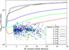 |
Fig. 6. Same as Fig. 2, but as a function of the mixed-mode density 𝒩. |
| In the text | |
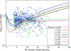 |
Fig. 7. Same as in Fig. 3, but as a function of the mixed-mode density. |
| In the text | |
|
Fig. 8. Core rotation rate as a function of the mixed-mode density for models during the hydrogen-shell burning phase. The efficiency of AM redistribution (parametrised by the additional viscosity νadd) varies in order to reproduce the mean evolution of the core rotation rate as given by asteroseismic constraints for a 1.5 M⊙ model with an initial period of Pini = 10 days at three different locations (𝒩 = 4, 9, and 14), shown with yellow dots on the evolutionary tracks. The dotted lines show the interval in which ⟨Ωcore⟩/2π ∈ [600, 800] nHz. |
| In the text | |
|
Fig. 9. Additional viscosity needed to satisfy the rotational constraints of red giants in the hydrogen-shell burning phase, normalised to its value at a mixed-mode density of 𝒩 = 4, as a function of the mixed-mode density. The different curves correspond to different initial masses, as indicated in the legend. |
| In the text | |
|
Fig. 10. Evolution of the core rotation rate as a function of the stellar radius. All models have an initial mass of 1.2 M⊙ and an initial velocity of 5 km s−1 (Pini = 12 days) and were computed with qcrMESA. Different values for the additional viscosity are used in each model, as indicated in the figure in units of cm2 s−1. The sharp drop in core rotation rate seen at R ∼ 150 R⊙ occurs because of the helium flash. The data correspond to red giants and red clump stars from Mosser et al. (2012). Only stars (data) with an estimated mass lower than M ≲ 2 M⊙ were included. Red clump stars are grouped at radii R ∼ 10 R⊙ (crosses), and red giants in the hydrogen-shell burning phase are located above this, with a higher core rotation rate and lower radii (circles). |
| In the text | |
|
Fig. 11. Same as Fig. 10, but for models with different initial masses, as indicated in the legend. We show only the region around the stable core-helium burning phase. All models have an additional viscosity of νadd = 5 × 105 cm2 s−1. The data points correspond to red clump stars from Mosser et al. (2012). Dotted lines: before stable core-helium burning. Solid lines: long and stable core-helium burning phase (see text). Dash-dotted lines: last fraction of the stable core-helium burning phase. |
| In the text | |
|
Fig. 12. Evolution of the efficiency of AM redistribution, parametrised by the additional viscosity νadd, as a function of the radius normalised to the radius at the end of the MS. Black dots with R/RTAMS < 2 correspond to subgiants studied by Deheuvels et al. (2020) and Eggenberger et al. (2019b). The other symbols correspond to red giants in the phase of hydrogen-shell burning with different initial masses and finally to the estimate for red clump stars based on a 1.2 M⊙ model. |
| In the text | |
Current usage metrics show cumulative count of Article Views (full-text article views including HTML views, PDF and ePub downloads, according to the available data) and Abstracts Views on Vision4Press platform.
Data correspond to usage on the plateform after 2015. The current usage metrics is available 48-96 hours after online publication and is updated daily on week days.
Initial download of the metrics may take a while.