| Issue |
A&A
Volume 663, July 2022
|
|
|---|---|---|
| Article Number | A79 | |
| Number of page(s) | 32 | |
| Section | Planets and planetary systems | |
| DOI | https://doi.org/10.1051/0004-6361/202243099 | |
| Published online | 18 July 2022 | |
Meta-modelling the climate of dry tide-locked rocky planets
1
IMCCE, Observatoire de Paris, Université PSL, CNRS, Sorbonne Université, Université de Lille,
75014
Paris, France
e-mail: pierre.auclair-desrotour@obspm.fr
2
University of Bern, Center for Space and Habitability,
Gesellschaftsstrasse 6,
3012
Bern, Switzerland
3
University of Warwick, Department of Physics, Astronomy & Astrophysics Group,
Coventry
CV4 7AL,
UK
4
Ludwig Maximilian University, University Observatory Munich,
Scheinerstrasse 1,
Munich
81679,
Germany
Received:
12
January
2022
Accepted:
25
March
2022
Context. Rocky planets hosted by close-in extrasolar systems are likely to be tidally locked in 1:1 spin-orbit resonance, a configuration where they exhibit a permanent dayside and nightside. Because of the resulting day-night temperature gradient, the climate and large-scale circulation of these planets are strongly determined by their atmospheric stability against collapse, which designates the runaway condensation of greenhouse gases on the nightside.
Aims. To better constrain the surface conditions and climatic regime of rocky extrasolar planets located in the habitable zone of their host star, it is therefore crucial to elucidate the mechanisms that govern the day-night heat redistribution.
Methods. As a first attempt to bridge the gap between multiple modelling approaches ranging from simplified analytical greenhouse models to sophisticated 3D general circulation models (GCMs), we developed a general circulation meta-model (GCMM) able to reproduce the closed-form solutions obtained in earlier studies, the numerical solutions obtained from GCM simulations, and solutions provided by intermediate models, assuming the slow rotator approximation. We used this approach to characterise the atmospheric stability of Earth-sized rocky planets with dry atmospheres containing CO2, and we benchmarked it against 3D GCM simulations using the THOR GCM.
Results. We observe that the collapse pressure below which collapse occurs can vary by ~40% around the value predicted by analytical scaling laws depending on the mechanisms taken into account among radiative transfer, atmospheric dynamics, and turbulent diffusion. Particularly, we find (i) that the turbulent diffusion taking place in the dayside planetary boundary layer (PBL) globally tends to warm up the nightside surface hemisphere except in the transition zone between optically thin and optically thick regimes, (ii) that the PBL also significantly affects the day-night advection timescale, and (iii) that the slow rotator approximation holds from the moment that the normalised equatorial Rossby deformation radius is greater than 2.
Key words: planets and satellites: atmospheres / planets and satellites: terrestrial planets / methods: numerical
© P. Auclair-Desrotour et al. 2022
 Open Access article, published by EDP Sciences, under the terms of the Creative Commons Attribution License (https://creativecommons.org/licenses/by/4.0), which permits unrestricted use, distribution, and reproduction in any medium, provided the original work is properly cited.
1 Introduction
Launched recently from Kourou’s spaceport in French Guiana, the James Webb Space Telescope (Deming et al. 2009) is on the point of unravelling the features of exoplanetary atmospheres at resolutions never before reached. With the current or upcoming transit searches of the TESS (Barclay et al. 2018) and PLATO (Ragazzoni et al. 2016) observatories, this telescope will accelerate the dynamics initiated by previous space missions by populating the continuum of extrasolar planets and constraining the properties of the detected objects. Many of these planets are rocky planets in close-in star–planet systems, notably planets that orbit brown dwarfs and very low-mass stars (e.g. Payne & Lodato 2007; Raymond et al. 2007; Kopparapu et al. 2017) such as the seven Earth-sized planets hosted by the TRAPPIST-1 ultra-cool dwarf star (Gillon et al. 2017; Grimm et al. 2018). Therefore, it is crucial to better understand the mechanisms governing their climate, atmospheric circulation, and surface conditions.
Tidal locking in 1:1 spin–orbit resonance is the most probable final spin state of planets in close-in star-planet systems (Goldreich 1966). This evolution results from the action of the gravitational tides raised by the perturbing tidal potential of the star. Because of dissipative mechanisms, the tidal response of the planet is delayed with respect to the perturber. As a consequence, the resulting tidal torque tends to drive the spin towards the configuration where the star is motionless in the frame of reference rotating with the planet. This spin state corresponds to spin-orbit synchronisation and is reached when the spin angular frequency of the planet, Ω, equalises its orbital frequency, n⋆.
Additionally, gravitational tides act to decrease both the obliquity and the eccentricity of the planet, which is thereby driven towards the equilibrium configurations of coplanarity and circularity (Hut 1980, Hut 1981) unless it spirals towards the star until being engulfed by it if the system is very close (Hut 1981; Levrard et al. 2009). Asynchronous final spin states may also exist. For instance, eccentric orbits maintained by orbital resonances in a multiple-planet system lead to spin-orbit resonances of higher degrees where the planet can be trapped (Correia et al. 2014; Auclair-Desrotour et al. 2019a). Similarly, it has been shown that significant thermal tides generated by stellar irradiation are able to prevent Venus-like planets from reaching spin–orbit synchronisation by inducing a torque opposed to the solid tidal torque (Gold & Soter 1969); Ingersoll & Dobrovolskis 1978; Leconte et al. 2015; Auclair-Desrotour et al. 2019b).
The probability of a planet being tidally locked in 1:1 spin– orbit resonance with temperate surface conditions is determined from the interplay between two radii: the tidal-lock radius, rT, and the radius of the habitable zone, rHZ. While the tidal-lock radius indicates the size of the region where planets are likely to be tide-locked in spin–orbit synchronisation, the radius of the habitable zone corresponds to the typical star-planet distance at which a planet can sustain liquid water at its surface (Kopparapu et al. 2013). By assuming that the planet behaves as a black body, and by writing the stellar luminosity as a function of the stellar mass with the empirical formula given by Barnes et al. (2008), it can be shown that  (Auclair-Desrotour & Heng 2020), whereas the tidal-lock radius scales as
  (Peale 1977; Kasting et al. 1993; Dobrovolskis 2009; Edson et al. 2011). Thus, the size of the habitable zone radius decays faster than the tidal-lock radius with decreasing stellar mass, which means that planets located in the habitable zone have a greater chance of being tide-locked if they orbit low-mass stars than if they orbit Sun-like stars (Kasting et al. 1993).
For planets orbiting low-mass M stars, tide-locking times are actually very short, and even extremely short in the case of lava planets (e.g. 55 Cancri e, Kepler 10b), with maximum values reaching just a few million years. For instance, the time required for the cool planet LHS1140 b to become tide-locked is about 14 million years (Pierrehumbert & Hammond 2019), which is low compared with the typical ages of planetary systems. This strongly suggests that planets orbiting in the habitable zone of very low-mass stars such as TRAPPIST 1d are tide-locked in the 1:1 spin–orbit resonance. Therefore, the rotation rate of these planets is well constrained and is given by Ω = n⋆. Additionally, the strength of tidal forces makes the existence of orbital configurations with significant eccentricities or obliquities unlikely. Such planets can thus be reasonably supposed to be close to the stable equilibrium configurations of coplanarity and circularity.
In this configuration, the planet exhibits a permanent day-side and nightside centred on the star–planet axis. The dayside is irradiated by the incident stellar flux while the nightside is radiatively cooled, and the energy absorbed on the dayside is transported towards the nightside by mean flows, which act to decrease the horizontal temperature gradient (e.g. Showman & Guillot 2002; Leconte et al. 2013; Pierrehumbert & Hammond 2019). The differential thermal forcing induced by spin–orbit synchronisation plays a crucial role in the evolution of the planet’s climate. Typically, as shown by the pioneering work of Joshi et al. (1997), the thermal state of synchronously rotating rocky planets is determined by the interplay between the night-side surface temperature and the condensation temperature of greenhouse gases. From the moment that the condensation temperature of the gas exceeds the surface temperature, the nightside acts as a cold trap. The greenhouse gas initially present in the atmosphere condenses and forms an ice sheet on the surface, which induces a temperature decrease in return. This triggers a positive feedback that cools down the atmosphere until the gas has been fully condensed, which is called atmospheric collapse (e.g. Joshi et al. 1997; Heng & Kopparla 2012; Wordsworth 2015). In the opposite case, the atmosphere is said to be stable against collapse, its composition remaining unchanged.
Over the past decade, a substantial effort has been made to characterise the climate of tide-locked rocky planets using a broad range of modelling approaches, from simplified analytical greenhouse models (e.g. Heng & Kopparla 2012; Wordsworth 2015; Auclair-Desrotour & Heng 2020) to 3D general circulation model (GCM) simulations (e.g. Merlis & Schneider 2010; Leconte et al. 2013; Carone et al. 2014; Haqq-Misra et al. 2018; Ding & Pierrehumbert 2020; Sergeev et al. 2020; Turbet et al. 2018), including intermediate semi-analytical or numerical approaches (e.g. Yang & Abbot 2014; Koll & Abbot 2016; Song et al. 2021) that cannot be listed here in an exhaustive way. Although based on robust methodologies, most of these approaches cannot be related self-consistently to one anotherdue to major differences in modelling choices. These discrepancies raise the two questions of how to disentangle the possible causes of different predictions between two models and how to assess the epistemic value of a given model. They can be reformulated into the more concrete question of how to consistently characterise the climate of tide-locked planets from multiple modelling approaches. This major concern was explicitly formulated by Held (2005), who argued for the need of model hierarchies on which to base one’s understanding in climate modelling. Such hierarchies appear as the only way to close the gap between idealised modelling and high-end simulations as they allow the essence of each particular source of complexity to be captured.
The aim of the present work is to tackle these questions from the angle of atmospheric stability against collapse. In the continuity of a former study on the atmospheric stability of tide-locked rocky planets (Auclair-Desrotour & Heng 2020), we have developed a multi-dimensional model hierarchy that we call a general circulation meta-model (GCMM) in order to bridge the gap between the analytic theory of planetary climates and simulations performed with 3D GCMs. This model hierarchy is based on a systematic bottom-up approach in the spirit of Held (2005).
We need to specify the sense given here to meta-modelling. By meta-model, we mean that the model ought to be able to exactly reproduce the setups of both simplified greenhouse models and GCMs – as well as the configurations in between – with the same intrinsic theoretical background. In that sense, such models are possible instances of the meta-model, which can generate any of them. Hence, the so-defined GCMM allows the effects of mechanisms that are either strongly coupled in standard GCMs or ignored in simplified analytic models to be disentangled. These effects are added or subtracted as a function of the number of degrees of freedom of the model. Increasing the number of degrees of freedom amounts to adding key sources of complexity.
Typically, radiative 0D models are essentially based on radiative exchanges between the planet’s surface and the atmosphere (e.g. Wordsworth 2015; Auclair-Desrotour & Heng 2020). At the next level of complexity, 1D models take the coupling between radiative transfer and the atmospheric structure into account (e.g. Robinson & Catling 2012). Two-column – or 1.5D – models are the minimum setup to self-consistently couple the large-scale day-night overturning circulation with radiative transfer and the atmospheric structure (e.g. Yang & Abbot 2014; Koll & Abbot 2016). This coupling is refined at the level of 2D GCMs, which allow the interaction between physical mechanisms – clouds, turbulent diffusion in the planetary boundary layer (PBL), convection – and mean flows to be calculated self-consistently in the slow rotation regime (e.g. Song et al. 2021). Finally, 3D GCMs complete the picture by introducing Coriolis effects and non-axisymmetric flows where super-rotation can develop (e.g. Leconte et al. 2013; Carone et al. 2014; Haqq-Misra et al. 2018; Ding & Pierrehumbert 2020; Sergeev et al. 2020; Turbet et al. 2021).
Thus, the essential function of a GCMM is to model all these levels of complexity at the same time so that the roles played by the different mechanisms involved in the planet’s climate can be clearly separated. As, to our knowledge, such a model has not yet been developed, the present work is a first attempt to design a GCMM dedicated to the study of tide-locked rocky planets. For simplicity, we confine ourselves to the slow rotation regime and ignore Coriolis effects in the dynamics. This allows us to avoid the mathematical complications related to the 3D geometry and to speed up calculations. Our GCMM is thus designed to generate models ranging from 0D configurations to 2D configurations. Additionally, we opt for a finite-volume method to solve the hydrostatical primitive equations (HPEs), following the approaches detailed by Yao & Stone (1987) and implemented in standard finite-volume GCMs such as the LMDZ (Hourdin et al. 2006) or THOR (Mendonça et al. 2016) GCMs. As the finite-volume method divides the atmosphere into cells, it is appropriate to describe the radiative energy balance models on which the analytic theory is built. For instance, the one-cell configuration (1 × 1 grid) corresponds to the single-layer isothermal atmosphere of Wordsworth’s model (Wordsworth 2015). Similarly, increasing numbers of horizontal and vertical grid intervals generate the 1D (1 × 50 grid), 1.5D (2 × 50 grid), and 2D (32 × 50 grid) model setups.
In order to minimise the size of the parameter space, we confine ourselves to the dry case in this study. The effects of moisture (clouds, latent heat transport, sedimentation, and surface condensation or evaporation) are ignored. Radiative transfer is described in the double-grey approximation, meaning that the fluxes are divided into two bands – shortwave and longwave – characterised by effective absorption parameters (e.g. Sect. 4.1 of Heng 2017). We also make the two-stream approximation and consider that radiative fluxes only travel upwards and downwards (e.g. Heng 2017, Sect. 3.1). In addition to radiative transfer, the vertical turbulent diffusivity induced by the interactions between mean flows and the planet surface in the PBL is taken into account by making use of a model based on the mixing length theory (Holtslag & Boville 1993). Finally, the thermal diffusion in the soil is included in the diffusion scheme of the GCMM with a 1D finite-difference model following the method described by Wang et al. (2016). As shown by earlier studies (Wordsworth 2015; Koll & Abbot 2016; Auclair-Desrotour & Heng 2020), the three abovementioned physical ingredients (circulation, radiative transfer, and turbulent diffusion) predominantly determine the nightside surface temperature and, thereby, the atmospheric stability against collapse. Table 1 summarises the physics described by the studied instances of the meta-model and the THOR 3D GCM, with the latter used to benchmark the former. Physical mechanisms are gradually captured by the grid formats that characterise the models as the number of degrees of freedom increases.
In Sect. 2, we introduce some of the control parameters and analytical scaling laws that characterise the climate and circulation regime of tide-locked planets. In Sect. 3 we detail the main features of the GCMM and the physical setup of the studied Earth-like and pure CO2 atmospheres. Section 4 introduces the four instances of the meta-model used in this work: 0D, 1D, 1.5D, and 2D. In Sect. 5, we run grid simulations for these instances to characterise the atmospheric stability of Earth-sized synchronous planets against collapse as a function of the stellar flux and surface pressure. Particularly, this vertical inter-comparison highlights the influence of the PBL on climate, day-night advection, and surface conditions. In Sect. 6, we investigate the limitations of the zero-spin rate approximation assumed in this approach by running simulations with the THOR 3D GCM. We show that the approximation holds from the moment that the dimensionless equatorial Rossby deformation length is greater than 2. Finally, in Sect. 7 we summarise the conclusions of the study.
Physics described by the four studied instances of the meta-model and the THOR 3D GCM.
2 Preliminary scalings
The circulation regime and thermal state of equilibrium of tide-locked planets is controlled by a few parameters and scaling laws derived either from the shallow water approximation (e.g. Vallis 2006; Pierrehumbert & Hammond 2019) or from the weak temperature gradient (WTG) approximation (e.g. Pierrehumbert 1995; Sobel et al. 2001). One ought to recall these scalings before introducing the physical setup of the numerical approach.
2.1 Circulation regimes of synchronous planets
If we assume that the planet surface is isotropic, all the physics and dynamics that govern the atmospheric circulation are symmetric about the star–planet axis except Coriolis terms. As a consequence, the circulation regime is essentially characterised by one control parameter depending on the planet’s spin angular velocity, which determines whether mean flows are bidimensional and symmetric about the star–planet axis or if they are sufficiently deviated by the planet’s rotation as to become 3D.
Such a parameter appears naturally in analyses making use of the Buckingham-Pi theorem (Buckingham 1914) in the primitive equations of fluid dynamics and thermodynamics (e.g. Koll & Abbot 2015). In the present study, following Leconte et al. (2013) and Auclair-Desrotour & Heng (2020), we define the dimensionless equatorial Rossby deformation length  from the equatorial Rossby deformation radius LRo as (e.g. Menou et al. 2003)
 (1)
(1)
where Rp designates the planet radius, and cwave the speed of horizontally propagating gravity waves. The dimensionless equatorial Rossby deformation length is essentially the square root of the distance – in radius unit – that fast gravity waves can travel before they feel the Coriolis effects and geostrophically adjust (Vallis 2006).
If  , the Coriolis effects are small and the two-way force balance between advection and pressure-gradient accelerations leads to a day-night overturning circulation symmetric about the star–planet axis (Leconte et al. 2013; Pierrehumbert & Hammond 2019; Hammond & Lewis 2021). In this regime, the dynamics of mean flows is the same in all planes containing the star–planet axis, with high-altitude winds blowing from the day-side to the nightside and near-surface winds blowing from the nightside to dayside. This essentially corresponds to the steady state expected in the WTG theory, where small Coriolis forces, friction, and non-linearities make the heat advection unable to annihilate completely the day-night temperature gradient (Sobel et al. 2001; Hammond & Pierrehumbert 2017; Pierrehumbert & Hammond 2019).
Conversely, for  , Showman & Polvani (2011) demonstrated that the formation of standing planetary-scale equatorial Rossby and Kelvin waves (i.e. waves restored by the Coriolis acceleration; see e.g. Lee & Saio 1997) favours the emergence of super-rotation by pumping angular momentum from the mid-latitudes towards the equator. In this regime, the equatorial Rossby deformation radius (LRo) essentially corresponds to the latitudinal width of the produced eastward equatorial jet, and mean flows take the form of the Matsuno-Gill standing wave pattern (Matsuno 1966b; Gill 1980; Showman & Polvani 2011; Tsai et al. 2014).
The dimensionless equatorial deformation length introduced in Eq. (1) can be related to the atmospheric parameters by considering the properties of gravity waves. Gravity waves are restored by the Archimedean force associated with the fluid buoyancy and their typical speed is given by cwave = HN, where H designates the characteristic vertical scale length of the atmosphere and N the Brunt-Vaisala frequency, which scales the strength of the atmospheric stratification against convection (Gerkema & Zimmerman 2008). In a dry, stably stratified atmosphere, this frequency is expressed as (Gerkema & Zimmerman 2008)
 (2)
(2)
where we have introduced the gravity g, the heat capacity per unit mass of the gas Cp, the temperature T, and the partial derivative operator over the altitude  . In the idealised case of the vertically isothermal atmosphere (constant temperature),
  , and the vertical scale is the pressure height (Vallis 2006, Sect. 1.4),
 (3)
(3)
where Rd ≡ RGP/Ma designates the specific gas constant for dry air, RGP being the ideal gas constant and Ma the mean molecular weight of the atmosphere. Thus, in this configuration (e.g. Leconte et al. 2013),
 (4)
(4)
which highlights the fact that the circulation regime depends on the planet’s spin rotation, thermal state, and atmospheric composition.
The dimensionless equatorial Rossby deformation length conveys exactly the same information as the WTG parameter Λ introduced in the WTG theory (see e.g. Pierrehumbert & Hammond 2019), which is defined as the Rossby radius of deformation – distinct from the equatorial deformation radius – normalised by the planet radius (Vallis 2006, Sect. 3.8.2). The two parameters are linked together by the relationship  (Pierrehumbert & Hammond 2019), meaning that either the former or the latter can be chosen to characterise the circulation regime. In the present study, we confine ourselves to the configuration of the WTG theory
  and consider thereby that mean flows are symmetric about the star–planet axis.
In addition with the slow and fast rotators regimes, there exists a third dynamical state that is proper to intermediate stellar cases in the range of 3000–3300 K and that is described as the Rhines rotation regime (Haqq-Misra et al. 2018; Sergeev et al. 2020). This regime is related to the Rhines length, which determines the maximum extent of zonally elongated turbulent structures (Rhines 1975). It occurs when the non-dimensional Rossby deformation radius is greater than one but the non-dimensional Rhines length is less than one (Haqq-Misra et al. 2018). The slow rotation and fast rotation regimes occur when both the non-dimensional Rhines length and Rossby deformation radius are greater than or less than one, respectively. The Rhines rotation regime is not considered here, meaning that we focus on the configuration where both the non-dimensional Rhines length and Rossby deformation radius are greater than one.
2.2 Thermal states predicted by radiative box models
Over the past decade, analytic solutions and scalings characterising the thermal state of equilibrium of tide-locked planets have been obtained both for hot Jupiters (Komacek & Showman 2016); Zhang & Showman 2017; Koll & Komacek 2018), lava planets (Hammond & Pierrehumbert 2017), and cooler rocky planets orbiting in the habitable zone of their host star (Showman et al. 2013; Wordsworth 2015; Koll & Abbot 2016; Pierrehumbert & Ding 2016; Koll 2022; Auclair-Desrotour & Heng 2020). Most of them were derived in the framework of the WTG theory and involve simplified atmospheric physics and structure. The present study builds on these works, and particularly those based on box model approaches, where the atmosphere and surface are reduced to large-scale energy reservoirs exchanging heat with each other (Wordsworth 2015; Koll & Abbot 2016; Auclair-Desrotour & Heng 2020). Although they are based on strong simplifications (isothermal atmosphere, large-scale averages, no self-consistent coupling between the dynamics and the thermodynamics), these models provide scalings that capture the behaviour of the thermal state of tide-locked rocky planets with a minimum set of physical parameters. Particularly, they lead to closed-form solutions for the nightside surface temperature Tn, which determines the whole atmospheric stability against collapse.
By considering a globally isothermal atmosphere interacting with dayside and nightside surface hemispheres, Wordsworth (2015) shows that the pure radiative equilibrium of the surface-atmosphere system corresponds, in the optically thin layer approximation (i.e. transparent in the visible and optically thin in the infrared), to the nightside temperature scaling (Wordsworth 2015, Eq. (29))
![${T_{{\rm{n;low}}}} \equiv {T_{{\rm{eq}}}}{\left[ {{1 \over 2}\left( {1 - {A_{\rm{s}}}} \right){\tau _{{\rm{s;L}}}}} \right]^{{1 \over 4}}},$](/articles/aa/full_html/2022/07/aa43099-22/aa43099-22-eq14.png) (5)
(5)
which can be generalised to optically thick atmospheres with scattering (Auclair-Desrotour & Heng 2020). In the above expression, As designates the surface albedo in the shortwave, τs;L the longwave optical depth at planet’s surface, and Teq the black body equilibrium temperature, which is defined as
 (6)
(6)
with F⋆ the incident stellar flux and σSB = 5.670367 × 10⁻⁸ W m−2 K−4 the Stefan-Boltzmann constant (Mohr et al. 2016).
Since it ignores all types of energy exchanges except radiative transfer, the estimate given by Eq. (5) can be interpreted as a lower bound for the nightside surface temperature of a rocky tide-locked planet. In reality, the strong convection generated by the thermal forcing of the atmosphere in the dayside PBL increases surface-atmosphere heat fluxes, which significantly affects the nightside temperature (Sergeev et al. 2020). The friction of the flow against the surface generates sensible heat exchanges in dry thermodynamics. Additionally, in moist atmospheres, surface evaporation generates latent heat exchanges, which results from the energy taken from or released in the fluid during the changes of phases of the component (Pierrehumbert 2010).
We consider here that the atmosphere is dry and thereby ignore the contribution of latent heat exchanges. Sensible heat exchanges can be introduced in the radiative box model by including, in the energy balance equations, the hemisphere-averaged sensible heat flux given by (e.g. Pierrehumbert 2010, Eq. (6.11), p. 396)
 (7)
(7)
where ρa is the atmospheric density at planet’s surface, CD the bulk drag coefficient characterising the strength of friction in the surface layer, and υsen the typical horizontal wind speed of the flow. Among these parameters, υsen accounts for the circulation, meaning that it cannot be self-consistently related to the thermal state of the system in this simplified approach. Nevertheless, it can be scaled from a dimensional analysis of the thermodynamic equation (e.g. Wordsworth 2015), or by making use of the heat engine theory (e.g. Koll & Abbot 2016; Koll & Komacek 2018; Auclair-Desrotour & Heng 2020). For instance, by modelling the overturning circulation as an ideal heat engine and using Carnot’s theorem (Bruhat 1968), Koll & Abbot (2016) found an upper bound of the dayside average surface wind speed (Koll & Abbot 2016, Eq. (12)),
![${\upsilon _{{\rm{sen}}}} = {\left\{ {\left[ {{T_{\rm{d}}} - {{\left( {1 - {A_{\rm{s}}}} \right)}^{{1 \over 4}}}{T_{{\rm{eq}}}}} \right]\left( {1 - {e^{ - {\tau _{{\rm{s;L}}}}}}} \right)\left( {1 - {A_{\rm{s}}}} \right){{{R_{\rm{d}}}{F_{\rm{*}}}} \over {2{C_{\rm{D}}}{p_{\rm{s}}}}}} \right\}^{{1 \over 3}}},$](/articles/aa/full_html/2022/07/aa43099-22/aa43099-22-eq17.png) (8)
(8)
which agrees well with the values obtained numerically from 3D GCM simulations (Koll & Abbot 2016); Koll & Komacek 2018).
For an isentropic cycle (i.e. an idealised Carnot’s heat engine), the weight of dayside sensible heating1 relative to radiative heating is controlled by the dimensionless parameter (Auclair-Desrotour & Heng 2020, Eq. (63))
![${L_{{\rm{sen}}}} \equiv {{2{C_p}{C_{\rm{D}}}{p_{\rm{s}}}} \over {{\tau _{{\rm{s;L}}}}{R_{\rm{d}}}{F_{\rm{*}}}}}{\left[ {{{{Q_{{\rm{in}}}}{R_{\rm{d}}}} \over {{C_{\rm{D}}}{p_{\rm{s}}}}}{{\left( {{{{F_{\rm{*}}}} \over {2{\sigma _{{\rm{SB}}}}}}} \right)}^{{1 \over 4}}}} \right]^{{1 \over 3}}},$](/articles/aa/full_html/2022/07/aa43099-22/aa43099-22-eq18.png) (9)
(9)
which is written here for an atmosphere optically transparent in the shortwave and thin in the longwave. The notation  (e.g. Koll & Abbot 2016) designates the amount of power per unit area available to drive atmospheric motion. Looking at the zero-convection limit (Lsen = 0) we recover the purely radiative regime, while the opposite asymptotic regime (Lsen = +∞) implies that Td = Ta and provides an upper bound for the night-side surface temperature of a tide-locked rocky planet (e.g. Auclair-Desrotour & Heng 2020, Eq. (85)),
![${T_{{\rm{n;up}}}} \equiv {T_{{\rm{eq}}}}{\left[ {2\left( {1 - {A_{\rm{s}}}} \right){\tau _{{\rm{s;L}}}}} \right]^{{1 \over 4}}} = \sqrt 2 {T_{{\rm{n;low}}}},$](/articles/aa/full_html/2022/07/aa43099-22/aa43099-22-eq20.png) (10)
(10)
which is valid in the optically thin layer approximation as well as Eq. (5). Therefore, for a globally isothermal and optically thin atmosphere, the nightside surface temperature falls into the interval
 (11)
(11)
However, we remark that Td = Ta actually corresponds to an extreme regime that is never reached in standard configurations, and we thus consider Tn;up as a theoretical upper limit.
Similarly as the dayside convective planetary layer, the nightside atmospheric structure alters the nightside equilibrium temperature. Its effect can be quantified by relaxing the isothermal approximation and by dividing the atmosphere into dayside and nightside air columns, which is the essence of two-column models (Yang & Abbot 2014); Koll & Abbot 2016; Auclair-Desrotour & Heng 2020). As shown by Koll & Abbot (2016), the nightside subsidence induced by the day-night overturning circulation generates a temperature inversion in the lowest layers of the atmosphere if the subsidence timescale is slightly greater than the radiative cooling timescale. The resulting atmospheric structure leads to large day-night differences.
3 A general circulation meta-model (GCMM)
We introduce in this section the main features of the meta-model and the used physical setup.
3.1 Primitive equations
At a given time, t, the dynamical core of the GCMM solves the HPEs over the Cartesian rectangular domain defined by the colatitude θ ∈ [0°, 180°] of the tidally locked coordinates (TLCs; see Koll & Abbot 2015, Appendix B) and the mass-based vertical coordinate defined, in the absence of the topography, as (e.g. Yao & Stone 1987; Carone et al. 2014)
![$\sigma \equiv {{p - {p_{\rm{t}}}} \over {{p_{\rm{s}}} - {p_{\rm{t}}}}} \in \left[ {0,1} \right],$](/articles/aa/full_html/2022/07/aa43099-22/aa43099-22-eq22.png) (12)
(12)
where we have introduced the pressure p, the surface pressure ps, and the pressure at the top of the atmosphere pt. In these coordinates, θ = 0° and θ = 180° correspond to the sub-stellar and anti-stellar points, respectively, while σ = 0 and σ = 1 correspond to the top and the bottom of the atmosphere, respectively. While ps and p vary over time and spatial coordinates, pt is set to pt = 0 in the model, which corresponds to the usual sigma coordinate σ = p/ps. The vertical coordinate given by Eq. (12) is well suited to the study of the tide-locked planets since it follows the distortion of the atmosphere induced by the differential day-night thermal forcing: the pressure of an altitude level may differ by orders of magnitude between the dayside and nightside, which would possibly generate numerical issues with the altitude coordinate.
The relationship between the altitude (z) and the generalised vertical coordinate (σ) is contained in the so-called pseudodensity (e.g. Kasahara 1974),
 (13)
(13)
where ρ denotes the density. The pseudo-density is proportional to the mass contained in a generalised volume where the vertical dimension is not a length but an interval of the generalised coordinate σ. With the chosen mass-based coordinate (Eq. (12)) and the assumed hydrostatic balance, it is simply expressed as (e.g. Yao & Stone 1987)
 (14)
(14)
We note that p would be the density to a constant factor if the vertical coordinate were the altitude. Using the pseudo-density instead of the density allows the HPEs given further in the same form to be written for any chosen vertical coordinate.
The HPEs are the mass continuity equation (e.g. Kasahara 1974),
 (15)
(15)
the horizontal momentum equation,
![$\matrix{ {{\partial \over {\partial t}}\left( {{\upsilon _\theta }\sin \theta } \right) + {1 \over {{R_{\rm{p}}}}}{\partial \over {\partial \theta }}\left( {\upsilon _\theta ^2\sin \theta } \right)} \hfill \cr { + {\partial \over {\partial \sigma }}\left( {{\upsilon _\theta }\dot \sigma \sin \theta } \right) + {1 \over {{R_{\rm{p}}}}}\sin \theta \left[ {{{\partial \phi } \over {\partial \theta }} + \Theta {{\partial E} \over {\partial \theta }}} \right] = \sin \theta {F_\theta }.} \hfill \cr } $](/articles/aa/full_html/2022/07/aa43099-22/aa43099-22-eq26.png) (16)
(16)
the potential temperature equation,
 (17)
(17)
and the hydrostatic equation combined with the ideal gas law,
 (18)
(18)
where we have introduced the horizontal velocity vector υσ ≡ υθ eθ, the sigma-velocity  (with
(with  the material time derivative), the geopotential ϕ ≡ gz, the potential temperature Θ, the Exner function E (e.g. Vallis 2006, Sect. 3.9), and the horizontal divergence operator at constant σ,
 (19)
(19)
The potential temperature and Exner function are defined as
 (20)
(20)
where T is the temperature, pref a constant reference pressure set to pref = 1 bar, and κ ≡ Rd/Cp. We note that the Exner function is a proxy for pressure. It is used for convenience, as it facilitates the integration of the hydrostatic equation. In right-hand members of Eqs. (15)–(18), the source-sink terms are the force per unit mass and the heat power per unit mass Q. We note that the primitive equations are written in their conservative forms, which involve mass flows and mass-integrated quantities rather than the original quantities themselves. Besides, these equations are given here for any vertical coordinate varying monotonically with altitude for the sake of generality.
The non-dimensional HPEs derived from Eqs. (15)–(18) (see Appendix A) are solved for {p, υθ, Θ, ϕ} on a staggered Arakawa C grid (Arakawa & Lamb 1977) with uniformly spaced horizontal intervals, and σ-dependent vertical intervals refined near the model bottom and top (see Appendix B). Following the method implemented in the LMDZ GCM (Hourdin et al. 2006), the integration is done using a leapfrog scheme with a periodic predictor/corrector timestep. The source-sink terms associated with the physics, {Fθ, Q}, as well as other physical variables, are updated periodically using implicit schemes except radiative transfer equations, which are solved directly from the current thermodynamical state. In the 2D GCM-like configurations, integrating the HPEs on a discrete domain generates numerical instabilities that develop at grid scale and may strongly disrupt calculations. In GCMs, this concern is usually handled by introducing horizontal hyper-diffusion, which is ideally designed to efficiently damp the numerical instabilities at grid scale while leaving the mean flows unchanged (e.g. Thrastarson & Cho 2011). Therefore, we include in the model a fourth-order hyper-diffusion (or bi-harmonic diffusion) using an anisotropic super-diffusivity that vanishes at the sub-stellar and anti-stellar points (see Appendix C.1) in order to avoid the stability concerns associated with isotropic diffusion near the poles (Sect. 13.3 of Lauritzen et al. 2011). The corresponding hyper-diffusion terms for the momentum and temperature equations are given by
 (21)
(21)
 (22)
(22)
where  designates the second-order horizontal hyper-Laplacian operator, α the anisotropy exponent (α = 1 in the model), and K4 the super-diffusivity defined by Eq. (C.5). Validation test simulations were run to verify that the mean flow and temperature distribution are insensitive to the hyper-diffusion scheme (see Fig. C.1).
In very hot cases, exponentially growing gravity waves propagating upwards and reflected by the upper boundary of the model can lead to extreme fluctuations of the dynamical quantities in the upper atmosphere. To address these instabilities, it can be necessary to use a sponge layer in addition with horizontal hyper-diffusion. In the present work, we introduce a linear Rayleigh friction sponge (e.g. Lauritzen et al. 2011, Sect. 13.4.5) following the formulation proposed by Polvani & Kushner (2002) for the vertical profile of the Rayleigh coefficient (see Appendix C.2). The sponge layer is thus modelled by a Rayleigh damping increasing with the altitude between a critical level σ = σSL and the top of the atmosphere, σ = 0, which tends to annihilate horizontal winds in the vicinity of the upper boundary. Finally, the strong convection generated by the thermal forcing on the dayside can induce super-adiabatic vertical temperature gradients (i.e. ∂Θ/∂z < 0), which is another source of numerical errors. This behaviour can be prevented by introducing a convective adjustment scheme in the model. The convective adjustment scheme regularises the atmospheric structure by dynamically correcting the tendencies to adjust super-adiabatic regions to adiabatic profiles. We implemented a standard scheme (e.g. Hourdin et al. 1993; Mendonça & Buchhave 2020) that can be activated when necessary (see Appendix D). However, we did not have to use the convective adjustment scheme nor the sponge layer in the simulations performed for this work.
3.2 Radiative transfer
In the model, radiative transfer is described through the double-grey approximation, which consists in (i) decoupling the stellar radiation (shortwave flux) and the planet radiation (longwave flux) – each band being characterised by an effective optical depth – and (ii) assuming that radiative fluxes only propagate upwards and downwards, which is the essence of the two-stream approximation (e.g. Heng 2017, Sects. 3.1 and 4.1). This allows fluxes in the shortwave and in the longwave to be calculated separately (see Appendix E). We denote upward and downward fluxes by F↑ and F↓ respectively. The equations governing the propagation of the wavelength-integrated total flux F− ≡ F↑ + F↓ and net flux F+ ≡ F↑ + F↓ have the same formulation in both bands. They are written as (Heng 2017)
 (23)
(23)
 (24)
(24)
where B ≡ σSBT4 designates the black body radiation of the gas, which is zero in the shortwave since the atmosphere is assumed to radiate in the infrared only.
In these equations, τ designates the optical depth of the associated band, and β0 the scattering parameter (β0 = 1 for pure absorption; 0 < β0 < 1 in the presence of scattering). The fluxes equations given by Eqs. (23) and (24) are solved numerically in the code by computing the transmission functions of each atmospheric layer as a first step, and by solving the boundary condition problem as a second step. We note that the solution obtained numerically for the single-layer atmosphere this way exactly corresponds to that derived in radiative box models based on the isothermal atmosphere approximation (see e.g. Wordsworth 2015; Auclair-Desrotour & Heng 2020). The optical depths in the shortwave τS and longwave τL are both assumed to scale linearly with pressure, and are defined as
 (25)
(25)
where we have introduced the effective absorption coefficients of the gas in the short- and longwave, κS and κL, respectively.
We remark that the optical depths defined by Eq. (25) depict horizontally averaged vertical profiles rather than local profiles varying as functions of the propagation angles of radiative fluxes, αS and αL. Therefore, the effective absorption coefficients κS and κL introduced in Eq. (25) are related both to the absorption properties of the gas and to the mean cosine of the propagation angles in the visible and in the infrared,  and
and  . Typically, these coefficients are related to Wordsworth’s absorption coefficients (Wordsworth 2015, Eq. (12)) – denoted by
  and
and  – by the equations2
  and
and  . Therefore, changing the value of the mean cosine of the propagation angle in this definition amounts to changing the value of the absorption coefficient in Eq. (25). One shall also bear in mind that the absorption coefficients defined in the double-grey approach are not fundamental parameters of the gas but parameters that mimic the averaged effect of highly frequency-dependent atmospheric opacities, as shown by Wordsworth et al. (2010a) for CO2-dominated atmospheres.
Although it does not fully account for the complex physics of radiative transfer, the adopted double-grey approximation with average optical depths captures the dependence of optical depths on pressure, and it allows for fast numerical computation of radiative fluxes. The radiative transfer scheme may be refined in future works by using more sophisticated approaches such as the correlated-k distribution method (e.g. Lacis & Oinas 1991), but this goes beyond the scope of the present study.
3.3 Planetary boundary layer
In the PBL the shear instability generates turbulence, which acts to mix the flow. This turbulent mixing induces a vertical diffusion of momentum, heat, and potentially moisture in moist cases, near the planet’s surface. The associated eddy diffusivities are controlled by the gradient Richardson number Ri defined as (Vallis 2006)
 (26)
(26)
which characterises fluid stratification. The Richardson number is essentially the ratio of the production of turbulent energy due to the shear instability over the restoring force induced by buoyancy. For a given quantity X = υθ, CpΘ (or q in moist cases, q being the specific humidity), the vertical diffusion equation is written, in the gradient-flux theory (e.g. Garratt 1994), as
![${{{\rm{d}}X} \over {{\rm{d}}t}} = {1 \over \rho }{\partial \over {\partial z}}\left[ {\rho {K_X}{{\partial X} \over {\partial z}}} \right],$](/articles/aa/full_html/2022/07/aa43099-22/aa43099-22-eq46.png) (27)
(27)
the upward diffusive flux being given by
 (28)
(28)
In these equations, KX is the eddy diffusivity associated with turbulent mixing for X. This parameter is a function of the mean fields. The lower boundary condition is a continuity condition determined by the exchanges with the planet’s surface, while the upper condition is a zero-flux condition. In a dry atmosphere, the tendencies for the momentum and potential temperature equations in the dry case are expressed from the diffusive terms given by Eq. (27) as
 (29)
(29)
To calculate the eddy diffusivities, we make use of the formulation given by Holtslag & Boville (1993). In that model, the eddy diffusivities of Eq. (27) are expressed as functions of a mixing length scale ℓ, the local shear  , and the gradient Richardson number Ri defined by Eq. (26). They read (e.g. Holtslag & Boville 1993, Eq. (3.2))
 (30)
(30)
where FX (Ri) describes the functional dependence of KX on the gradient Richardson number. The form of FX is determined by the turbulent regime, which can be either stable (Ri ≥ 0) or unstable (Ri < 0). The mixing length is expressed as (Blackadar 1962)
 (31)
(31)
the parameter K ≈ 0.4 being the von Karman constant (e.g. Garratt 1994), and ℓ0 the asymptotic length scale (ℓ ≈ ℓ0 for Kz ≫ ℓ0), which varies as a function of z (see Appendix F.1).
The turbulent friction of mean flows against the soil in the surface layer leads to sensible momentum and heat exchanges that are described in the form of parametrised surface fluxes. Denoting by M and H the subscripts for the momentum and heat components, respectively, we write the upward momentum and heat surface fluxes as
 (32)
(32)
 (33)
(33)
where the subscripts s and SL refer to values at the surface and at the top of the surface layer3, respectively. The surface-layer exchange coefficients CM and CH are defined as (Holtslag & Boville 1993)
 (34)
(34)
 (35)
(35)
Here, CN designates the neutral exchange coefficient (e.g. Holtslag & Boville 1993),
![${C_{\rm{N}}} \equiv {\left[ {{{\cal K} \over {{\rm{1n}}\left( {1 + {{{z_{{\rm{SL}}}}} \mathord{\left/{\vphantom {{{z_{{\rm{SL}}}}} {{z_{\rm{r}}}}}} \right.\kern-\nulldelimiterspace} {{z_{\rm{r}}}}}} \right)}}} \right]^2},$](/articles/aa/full_html/2022/07/aa43099-22/aa43099-22-eq56.png) (36)
(36)
where zr denotes the roughness height, while fM and fH are two functions of the bulk Richardson number,
 (37)
(37)
which controls the stability of the surface layer. We note that the bulk Richardson number Ri0 corresponds to the local gradient Richardson number Ri (Eq. (26)) characterising the surface layer. The functions fM and fH, as well as the functions FX introduced in Eq. (30), are detailed in Appendix F.1. The physical tendencies resulting from turbulent diffusion are evaluated every physical time step using an implicit scheme (see Appendix F.2).
As it accounts for the dependence of eddy diffusivities on the gradient Richardson number, the above turbulent diffusion scheme describes both the regime of strong convection occurring on the dayside and the regime of stable stratification associated with the nightside temperature inversion (see Figs. 1 and 2 in the following). It thus captures the evolution of turbulent diffusivities in the PBL between the dayside, where they are high, and the nightside, where they are low. However, we note that the used standard formulation of turbulent diffusion is not sophisticated enough to account properly for the heat and momentum exchanges due to turbulent flows in the case of strong stratification (Ri ≫ 1). In this regime, the vertical momentum mixing continues even at relatively high Ri due to the momentum transport of vertically propagating internal gravity waves, which may increase the surface-atmosphere sensible heat exchanges and warm up the nightside surface (e.g. Sukoriansky et al. 2005; Joshi et al. 2020). Considering this effect, the used turbulent scheme might tend to underestimate the atmospheric stability against collapse. Nevertheless, we adopt it as a convenient compromise between simplicity and realism, which can be refined in the future by using more advanced turbulent diffusion models (e.g. Sukoriansky et al. 2005).
3.4 Soil heat transfer
The soil heat transfer is solved by using a classical 1D soil heat conduction approach (e.g. Hourdin et al. 1993; Wang et al. 2016). The evolution of the ground temperature, T, due to vertical diffusion is governed by the heat equation
 (38)
(38)
where u = −z is the depth from surface (u ≥ 0), Cgr the heat capacity of the ground per unit volume, and Fc the conductive flux propagating downwards. The conductive flux is expressed as
 (39)
(39)
the parameter λgr being the thermal conductivity of the material. Both Cgr and λgr are assumed to be constants in the model.
We introduce the normalised pseudo-depth
 (40)
(40)
which has dimensions of s1/2. Expressed in terms of ũ, the vertical diffusion is controlled by one parameter solely, the thermal inertia
 (41)
(41)
The downward conductive flux given by Eq. (39) then becomes
 (42)
(42)
and the vertical diffusion equation simply reads
 (43)
(43)
The above equation is solved by means of the finite difference method between the surface (ũ = 0) and an inner boundary (ũ = ũbot) using an implicit time scheme. At the surface, a continuity condition is applied: the incoming heat fluxes equalise the outcoming fluxes. At the inner boundary, a zero-flux condition is applied, which enforces the assumption that the planet interior is in thermal equilibrium. These two conditions are respectively formulated as
 (44)
(44)
where F↓ designates the downward radiative flux (i.e. the sum of the shortwave and longwave contributions), F↑S the reflected shortwave flux, Ts the surface temperature, and εs the surface emissivity in the longwave. The scheme used to solve the soil heat transfer is detailed in Appendix G. Similarly as the radiative transfer and turbulent diffusion equations, the soil heat transfer equation is discretised and integrated as a boundary condition problem by means of the tri-diagonal matrix algorithm (see Appendix H).
Several simulations were run in order to assess the sensitivity of mean fields to the heat transfer scheme. The obtained results are discussed in Appendix G. They show that mean flows and temperatures do not depend much on the ground thermal inertia that parametrises the soil heat transfer scheme (Eq. (41)). Particularly, the nightside surface temperature is almost insensitive to the value chosen for Igr. Nevertheless, we recall that horizontal diffusion is ignored in the scheme since we focus of dry rocky planets, while it might play an important role for an ocean planet due to heat advection by oceanic flows, as discussed by Wordsworth (2015).
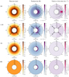 |
Fig. 1 Two-day averaged snapshots of pressure (left), temperature (middle), and vertical wind speed (right) distributions for the 1 bar-atmosphere of an Earth-sized tidally locked planet (Earth-like case of Table 2) with a stellar irradiation of 1366 W m−2 after convergence (t = 400 days). From bottom to top: OD (1 × 1 grid), 1D (1 × 50 grid), 1.5D (2 × 50 grid), and 2D (32 × 50 grid) instances of the meta-model. The sub-stellar point corresponds to θ = 0° and the anti-stellar point to θ = 180°. |
Values of parameters used in the two reference cases of the present work.
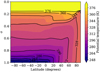 |
Fig. 2 Two-day averaged potential temperature field in the Earth-like case of Table 2 with ps = 1 bar and F⋆ = 1366 W m−2. Plotted values belong to the interval [248 K, 376 K]. Outside of this interval, the colour is set to that of the closest bound. The 2D instance of the meta-model (32 × 50 grid) is used. The latitudes 90° and −90° correspond to the sub-and anti-stellar points, respectively. |
3.5 Physical setup
In the following, we perform simulations for the two cases defined in Table 2: (i) and Earth-like atmosphere, and (ii) a pure CO2 atmosphere. For the Earth-like case, we use the values given by Deitrick et al. (2020) in the synchronous Earth case (see Deitrick et al. 2020, Table 2). These values correspond to a tide-locked Earth-sized planet with an atmosphere having the thermodynamical properties of the Earth’s atmosphere. Following Wordsworth (2015), we assume that τL = 1 at p = 1 bar. Similarly, we fix τS = 0.01 at p = 1 bar to enforce the assumption that the atmosphere is optically thin in the visible. The effective absorption coefficients introduced in Eq. (25) are set accordingly. Besides, we consider the case of pure absorption (no scattering). The scattering parameter is therefore set to β0 = 1 both for the shortwave and longwave. Assuming that the planet’s surface is made of bare rocks, we use the typical values commonly assumed for Venus-like soils (e.g. Lebonnois et al. 2010) to set the planet’s surface properties. Following Frierson et al. (2006), the roughness height is set to zr = 3.21 × 10⁻⁵ m so that CN = 10−3 for zSL = 10 m.
The pure CO2 case is similar to the Earth-like case except for the specific gas constant, Rd = 188.9 J kg−1 K−1 (calculated from Meija et al. 2016), the heat capacity per unit mass, Cp = 909.3 J kg−1 K−1 (evaluated for Τ = 350 Κ from Yaws 1996, Appendix E), and the absorption coefficient in the longwave, κL = 2.5 × 10⁻⁴ m2 kg−1. The latter is an effective value of κL for which the 2D instance of the GCMM presented in Sect. 4 approximately reproduces the stability diagram obtained by Wordsworth (2015) from 3D GCM simulations with correlated-k radiative transfer (Wordsworth 2015, Fig. 12), as shown in Sect. 5. We note that this value is less than that obtained by Wordsworth (2015) by adjusting the analytic solution given by Eq. (5) to GCM simulations (κL = 3.2 × 10⁻⁴ m2 kg−1 by taking into account the factor 2 difference between the definition of κL given by Eq. (12) of the article and ours, given by Eq. (25)). As highlighted by Sect. 5, this discrepancy is due to the fact that the PBL acts to warm up the nightside surface in the general case, which consequently requires a weaker greenhouse effect to reach the same thermal state.
4 Climate Regime: From 0D to 2D Models
The GCMM described in the preceding section can be used at the same time for various grid configurations, each of them being a possible instance of the meta-model. This allows the results obtained from a bench of models of various complexities, though with the same intrinsic theoretical background and physical setup, to be compared. Four instances of the meta-model are examined in the present study (Table 1). There are introduced below in ascending order of complexity, while the resulting pressure, temperature, and vertical wind speed snapshots are plotted in Fig. 1.
We note that, for legibility, the arrows representing wind speeds are uniformly spaced both horizontally and vertically in the figure, rather than being centred at the points where winds speeds are really evaluated. For instance, in the 1.5D model, the arrows are determined from a linear interpolation and located at θ = 45°, 135°, while horizontal wind speeds are evaluated at θ = 90°. In the range 180° < θ < 360°, the distributions are plotted by applying a symmetric transformation to the distributions calculated in the range 0° < θ < 180°. The additional inner ring in temperature snapshots (middle column of Fig. 1) corresponds to the soil temperature.
The 0D model (1 × 1 grid) is the simplest configuration. Here the atmosphere is vertically and horizontally isothermal, and it exchanges heat with dayside and nightside isothermal surface hemispheres through radiative transfer only. This configuration corresponds exactly to that of the two-layer grey radiative model described in Sect. 3 of Auclair-Desrotour & Heng (2020), which provides closed-form solutions. In the optically thin limit, it reproduces the analytic model introduced by Wordsworth (2015).
The next level of complexity is the 1D model (1 × 50 grid). In this configuration, the vertical structure of the atmosphere is allowed to adjust with radiative transfer although it is still horizontally isothermal. Similarly as in the 0D configuration, the planet’s surface is divided into the dayside and nightside hemispheres, and the surface-atmosphere heat exchanges are purely radiative. The 1D model thus provides a more realistic vertical temperature profile than that assumed in the 0D model. This profile can be interpreted as an approximation of the globally averaged atmospheric structure. This instance of the GCMM appears as a simplified version of more sophisticated 1D models (e.g. Robinson & Catling 2012).
Then we introduce the 1.5D model (2 × 50 grid). This level corresponds to the two-column approach, where the atmosphere is modelled by dayside and nightside hemispherical air columns, similarly as the planet’s surface (e.g. Yang & Abbot 2014; Koll & Abbot 2016). Therefore, the vertical structure ceases to be horizontally uniform and differences appear between the day-side and the nightside. However, these differences are mitigated by the fact that the dayside and nightside PBLs are both controlled by the horizontal wind speed at the planet’s terminator (θ = 90°) here, whereas horizontal wind speeds strongly differ between the dayside and nightside in reality. Besides, this configuration allows the coupling between the thermodynamics and the day-night overturning circulation to be taken into account, particularly the contribution of heat advection to the planet’s thermal state of equilibrium.
Finally, the 2D model (32 × 50 grid) is the more complex instance of the meta-model. In this configuration, the 2D model behaves similarly as a 2D GCM (e.g. Song et al. 2021) or a 3D GCM in the slow rotation regime (e.g. Leconte et al. 2013; Haqq-Misra et al. 2018; Pierrehumbert & Hammond 2019; Turbet et al. 2021). Both the atmospheric structure and mean flows are fully resolved, which describes the global heat engine circulation. The PBL strongly differs between the dayside, where it is unstable (Ri < 0) due to convection (see e.g. Koll & Abbot 2016), and the nightside, where it is stable (Ri ≥ 0). Also, the circulation is highly asymmetric with respect to the terminator: as shown by Fig. 1 (top panels), it exhibits strong upwelling flows in a small region around the sub-stellar point, and weak subsidence over a large area that spreads from θ ≈ 60° to θ = 180° (anti-stellar point).
We recover the day-night evolution of the atmospheric structure in the potential temperature distribution shown by Fig. 2, which was obtained using the 2D model. In this figure, the latitude is measured with respect to the terminator, located at 0°. The sub- and anti-stellar point thus correspond to the latitudes 90° and −90°, respectively. The nightside stably stratified region is characterised by a positive vertical potential temperature gradient. On the dayside, the convective mixing induced by the thermal forcing makes the temperature gradient converge towards the adiabat. As a consequence, convective regions are indicated by vertically uniform profiles of potential temperature. We note that the thickness of the PBL grows as the latitude increases, and that it is maximal at the sub-stellar point.
Owing to spatial bi-dimensionality, the solver is relatively fast even for the 2D instance, where one day of simulation with a two-minute dynamical timestep is equivalent to 0.61 seconds of CPU time on one CPU. This allows grid simulations to be run, which is the purpose of the next section.
5 Stability diagrams
In this section we examine both the role played by several physical features in the atmospheric stability, and the sensitivity of model predictions to the simplifications made in the different approaches. To do so, we proceed to a vertical inter-comparison between the four models introduced in Sect. 4 for the two Earth-sized synchronous planets defined in Table 2. For each instance of the meta-model, simulations were performed on a 15 × 13 grid in the space of stellar flux and initial surface pressure, with 0.2F⊕ < F⋆ < 3F⊕ and 0.01 bar ≤ ps ≤ 10 bar, F⊕ = 1366 W m−2 being the Earth’s incident stellar flux. Starting from isothermal and zero-velocity initial conditions, simulations were run for a period trun = min {max[trad, tmin], tmax} ranging between tmin = 300 and tmax = 30000 Earth days, trad being an empirical estimate of the timescale necessary to reach radiative equilibrium that includes the dependence of the radiative cooling timescale on surface pressure and stellar flux (e.g. Showman & Guillot 2002),
 (45)
(45)
At the end of simulations, two-day averaged distributions of mean fields were computed, as well as the resulting minimum (or nightside) surface temperature (Tn).
As highlighted by Wang & Wordsworth (2020) in the case of sub-Neptunes, the convergence time of 3D numerical simulations can be extremely long (trun ~ 250 000 Earth days, typically) for massive atmospheres (ps ≳ 80 bar) owing to the long radiative timescale of deep atmospheric layers. In the present study, the maximum surface pressure (10 bar) is smaller than that usually assumed for sub-Neptunes, the circulation described by our 2D model is simpler than that described by 3D GCMs – where complex structures and super-rotating zonal jets can emerge –, and the major part of the incident stellar flux reaches the planet’s surface, which tends to facilitate vertical energy transport. Therefore the resulting convergence times are expected to be smaller than those reached in the case of sub-Neptunes by one order of magnitude approximately. However, we verified a posteriori that both the energy balance between the outgoing longwave radiation and the absorbed stellar radiation on the one hand, and the circulation on the other hand, had reached a steady state at the end of several test simulations. Besides, by running grid simulations with larger values of trun, we noticed that increasing this parameter did not affect the considered mean fields.
Following earlier studies (Wordsworth 2015; Koll & Abbot 2016; Auclair-Desrotour & Heng 2020), we assume that the greenhouse effect is mainly due to the presence of CO2 in the atmosphere. The condensation temperature of CO2 is given, in K, by (Fanale et al. 1982; Wordsworth et al. 2010b; Wordsworth 2015)
 (46)
(46)
where the partial pressure of the gas p is given in Pa, and ptr = 5.18 × 10⁵ Pa designates the triple point pressure. The stability diagrams are therefore obtained by comparing the minimum surface temperature calculated from simulations with the condensation temperature of CO2 at the planet’s surface,  , where χ designates the volume mixing ratio of CO2. In the Earth-like case, the volume mixing ratio of CO2 is set to the value of Earth at the beginning of the 21st century, namely χ = 370 ppm (e.g. Etheridge et al. 1996), while χ = 1.0 in the pure CO2 case. The atmosphere is considered to be stable if
  and unstable else. We remark that the collapse itself, when it occurs, is not described by the model since the changes of phases of CO2 are not taken into account.
Figure 3 shows the simulation results. The minimum surface temperature is plotted in both cases as a function of the normalised stellar flux F⋆/F⊕ and the surface pressure ps in logarithmic scale. The stability diagrams are plotted too, with large red dots indicating stability and small blue dots collapse. The collapse pressures associated with the lower and upper bounds of the nightside temperature given by Eqs. (5) and (10), are obtained by solving for ps the equations
 (47)
(47)
 (48)
(48)
and are denoted by pC;low (orange dashed line) and pC;up (pink dotted line), respectively.
With the 0D model, we recover the behaviour of the nightside temperature predicted by the closed-form solutions of Auclair-Desrotour & Heng (2020) in the purely radiative regime. This is due to the fact that the two models are actually the same in this configuration, the temperatures being computed numerically here instead of analytically. Compared with the other models, the 0D model tends to underestimate the nightside temperature in the high surface pressure regime. As the surface pressure increases, Tn reaches a plateau that corresponds to the planet’s equilibrium temperature, Teq (F⋆), given by Eq. (6), and no longer evolves with ps. This unrealistic behaviour is a consequence of the isothermal approximation, which does not account for the strong vertical temperature gradient characterising thick atmospheres, especially their convective regions. In the low stellar flux regime, the 0D model captures the stability decrease observed for pure CO2 atmospheres in the 3D GCM simulations performed by Wordsworth (2015). However, this feature is due to the isothermal temperature profile too since it vanishes from the moment that the atmospheric structure is allowed to adjust with radiative transfer, in models of higher dimensions. This effect is a caveat of the limitations of idealised models in explaining predictions of much more sophisticated 3D GCMs.
The 1D model exhibits the same behaviour as the 0D model for surface pressures of less than 1 bar, which corresponds to the regime where the vertically isothermal approximation holds. Beyond ps ≈ 1 bar, the nightside surface temperature increases as a function of both the stellar flux and surface pressure, which makes the collapse pressure associated with Tn;low capture the threshold of the stability region for the whole stellar flux interval. The two-column configuration (1.5D model) relaxes the horizontally isothermal atmosphere approximation. As a consequence, the nightside temperature becomes dependent on the efficiency of the interhemispheric heat redistribution, and can thereby be less than the lower bound obtained in the horizontally isothermal atmosphere approximation, Tn;low. The coarse spatial resolution of the 1.5D model for the horizontal direction does not account for the strong convection generated in the sub-stellar region. The wind speed is therefore underestimated, and so are the strength of the overturning circulation and the heat advected from the dayside to the nightside. This leads to the observed stability decrease: the collapse pressure is approximately increased by ~25% with respect to pC;low in the Earth-like case, and by ~80% in the pure CO2 case.
Conversely, the 2D model predicts a wider stability region. The collapse pressure is lowered by ~ 10–40% with respect to pC;low for F⋆ ≳ 0.7F⊕, which is significant, albeit less than the 75% maximum decrease predicted by the analytic theory (pC;up/pC;low = 1/4; see Auclair-Desrotour & Heng 2020, Eq. (86)) in the case of intense sensible heating (Lsen → + ∞; see Eq. (9)). This stability increase results from the effect of the PBL. The vertical turbulent diffusion generated by the friction of mean flows against the planet’s surface in the planetary layer acts both (i) to increase the thermal forcing of the atmosphere by intensifying sensible exchanges, and (ii) to enhance the day-night heat advection by strengthening the overturning circulation. As a consequence, the nightside surface is warmer by ~4–14 K in the vicinity of the threshold between the stability and collapse regions.
The nightside temperature increase induced by the PBL was quantified by running simulations in the 2D configuration without turbulent diffusion both for Earth-like and pure CO2 atmospheres. In these simulations, the surface-atmosphere heat exchanges are induced by radiative transfer only, and there is no friction of mean flows against the surface. Figure 4 shows the resulting stability diagrams, as well as the corresponding night-side surface temperature difference between the cases with and without turbulent diffusion, denoted by the superscripts TD (turbulent diffusion) and NTD (no turbulent diffusion), respectively (top panels). In addition with the nightside surface temperature, we consider the day-night advection timescale tadv, which is defined here as the mean period necessary for a fluid parcel to accomplish one full cycle of the day-night overturning circulation (see Appendix I),
![${t_{{\rm{adv}}}} = {{4{R_{\rm{p}}}} \over {{{\left[ {\int_0^1 {\left| {{\upsilon _\theta }} \right|{\rm{d}}\sigma } } \right]}_{90^\circ }}}},$](/articles/aa/full_html/2022/07/aa43099-22/aa43099-22-eq71.png) (49)
(49)
where the subscript 90° indicates that the integral of the mass flow rate is performed over the terminator annulus (θ = 90°). The day-night advection timescale also corresponds to the mean renewal time of the air contained in one atmospheric hemisphere (dayside or nightside). This timescale can be compared to the advection timescales introduced in earlier studies, such as the analytic expression of the lower bound obtained by Koll & Abbot (2016) from the heat engine theory (Koll & Abbot 2016, Eq. (12)),
 (50)
(50)
where the typical speed υsen, given by Eq. (8), is a function of the stellar flux, the surface pressure, the surface albedo, the day-side surface temperature, the optical depth in the longwave at surface, the specific gas constant, and the bulk drag coefficient of the surface layer. The timescale  is estimated by setting the bulk drag coefficient to the typical value CD = 10−3 for convenience and by taking the maximum surface temperature for the dayside temperature. Thus, in addition with the nightside temperature difference mentioned above, we plot in Fig. 4 the day-night advection timescale in the case with turbulent diffusion (bottom panels), the ratio of this timescale over
  , and the ratio between advection timescales in the cases with and without turbulent diffusion (middle panels).
We first consider the stability diagrams obtained in the absence of turbulent diffusion (Fig. 4, top and middle panels). Similarly as in the ID configuration, the threshold of the stability region coincides with the lower bound of Tn associated with the purely radiative regime in the radiative box model, namely pC;low. This indicates that the bulk atmosphere is horizontally isothermal for ps ≳ 0.1 bar, which corresponds to an efficient interhemispheric heat redistribution. As highlighted by temperature differences (Fig. 4, top panels), turbulent diffusion tends to warm up the nightside surface in the general case with, for instance a temperature increase of 6–28 K in the Earth-like case. However, this temperature increase does not vary monotonically with the stellar flux and surface pressure, but instead it exhibits a bi-modal behaviour with maxima and minima depending on surface pressure.
Particularly, turbulent diffusion in the PBL somehow counter-intuitively acts to decrease the nightside surface temperature instead of increasing it in a region centred on ps ~ 1 bar for pure CO2 atmospheres, with a minimum of −8 K for ps = 1 bar and F⋆ = 1.2F⊕. A similar – although slightly smaller – negative difference (–5 K) was obtained by running grey gas simulations with the fully global 3D GCM THOR (Mendonça et al. 2016; Deitrick et al. 2020) in this configuration using the values given by Table 2 and assuming a zero-spin angular velocity, which tends to corroborate the prediction of the 2D model. This effect of the PBL can be analysed through the interplay between the day-night advection timescale given by Eq. (49) and the dayside radiative timescale, trad, which is the typical timescale needed for a warm fluid parcel located in the upper atmosphere to cool down radiatively. Both parameters are altered by the turbulent diffusion taking place within the PBL.
Notwithstanding the high pressure – and optically thick – regime, where strong convection develops, the effect of turbulent diffusion reaches a maximum around ps ~ 0.1 bar for Earth-like atmospheres and around ps ~ 0.03 bar for pure CO2 atmospheres (Fig. 4, top panels). This maximum is consistent with the fact that the additional thermal forcing due to turbulent diffusion is all the more significant as the radiative absorption is weak, which tends to maximise the impact of turbulent diffusion for small optical thicknesses. However, the radiative timescale of the atmosphere scales as  (e.g. Showman & Guillot 2002, Eq. (10)) in the optically thin regime, meaning that the heat surplus provided by sensible exchanges is radiated towards space over timescales that become extremely short as the surface pressure tends to zero. Thus, in spite of the decay of tadv induced by turbulent diffusion, a fluid parcel is radiatively cooled before being advected to the nightside by mean flows in the optically thin limit (trad ≪ tadv), which mitigates the impact of the PBL in this regime and makes the temperature difference decay as ps → 0.
Similarly, as the surface pressure increases, the atmosphere switches from the optically thin regime to the optically thick regime, with a transition occurring at lower pressures in the pure CO2 case than in the Earth-like case due to the difference between optical depths in the infrared. In this transition regime, the PBL strongly affects the advection timescale, which is increased up to three times (Fig. 4, middle panels) and becomes thereby greater than the radiative timescale. As a consequence, less heat is advected towards the nightside than in the absence of PBL – although the PBL generates a heat surplus on the dayside – and the nightside temperature difference falls to the observed minimum valley, where it reaches negative values in the pure CO2 case.
We note that this behaviour could be significantly altered by the presence of gas, dust, and aerosols inducing the so-called anti-greenhouse effect by increasing the shortwave scattering and absorption, as observed on Titan (McKay et al. 1991). The anti-greenhouse effect refers to the cooling of the planet surface resulting from the fact that a substantial part of the incident stellar flux is absorbed and re-radiated towards space in the infrared by the upper layers of the atmosphere, and that only a fraction of it reaches the surface (e.g. Pierrehumbert 2010). This effect is likely to play a major role on rocky planets with thick atmospheres similar to Venus, where only ~ 0.1–1% of the incident solar flux reaches the surface (Lacis 1975).
We now consider the evolution of the advection timescale itself, which is plotted in the case including turbulent diffusion in the PBL (Fig. 4, bottom panels). Similarly as the nightside surface temperature (Fig. 3), tadv exhibits a relatively smooth dependence on the incident stellar flux and surface pressure, with values spanning over two orders of magnitude from ~8 days in the low pressure-high stellar flux regime to ~500 days in the high pressure-low stellar flux regime. These values are larger than those given by the analytic scaling law of Koll & Abbot (2016) by one order of magnitude owing to the difference in the used definitions: since it is computed from the horizontal wind speed in the sub-stellar region, the analytic advection timescale is necessarily smaller than the advection timescale defined by Eq. (49), which is computed from mass flows going through the terminator annulus. Notwithstanding this scaling factor, matches relatively well for both Earth-like and pure CO2 atmospheres in the optically thin regime, where the ratio varies by a factor of two. The two quantities diverge from each other as the stellar flux decreases and the surface pressure increases, the model of the present study predicting larger advection timescales in this regime. However, we remark that this discrepancy is less significant for pure CO2 atmospheres than for Earth-like atmospheres, which suggests that the thermodynamic and absorption properties of the gas affect the large-scale overturning circulation in a non-negligible way when the atmosphere is optically thick.
The strength of the overturning circulation can be characterised by examining the behaviour of the Eulerian mean stream function, which is defined in TLCs as (e.g. Pauluis et al. 2008)
 (51)
(51)
The Eulerian mean stream function measures here the strength of longitude-averaged cells in the TLC. It accounts for the vor-ticity of the flow in a plane containing the planet-star axis. In the slow rotation regime, the large-scale cell of the predominant overturning circulation corresponds to a large region centred on a maximum of Ψ in absolute value, Ψ taking negative values owing to the flow direction (see e.g. Fig. 6 in the next section). The maximum value of Ψ over the atmospheric domain, defined as
 (52)
(52)
can be scaled analytically, as shown by Innes & Pierrehumbert (2022) who establishedforsub-Neptunes the scaling law 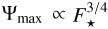 . In the case of rocky planets, we need to account for the presence of the planet’s surface, which sizes the thickness of the atmosphere. The mass flow thus depends on the atmospheric mass in addition with the stellar flux. As the atmospheric mass is directly proportional to the surface pressure, we introduce for rocky planets a scaling law of the form
 (53)
(53)
where T⊕ is the equilibrium temperature of Earth given by Eq. (6), pref = 1 bar a reference pressure, and α and β two real exponents to be defined. We remark that (α,·β) = (3/4, 0) corresponds to the scaling law obtained by Innes & Pierrehumbert (2022) for sub-Neptunes. However, for the Earth-sized rocky planets of the present study, we adopt the empirical values (α,β) = (1/2, 1), which seem to be more appropriate as discussed further.
Figure 5 shows the evolution Ψmax and of the ratio  as functions of instellation and surface pressure for the Earth-like and pure CO2 atmospheres defined in Table 2. In both cases the maximum of the Eulerian mean stream function varies over more than three orders of magnitude (Ψmax ~ 1010−1013 kg s−1), by increasing with F⋆ and ps monotonically. The scaling law given by Eq. (53) (with α = 1/2 and β = 1) approximately captures this behaviour although it can only be considered as a rough estimate of Ψmax. We observe that the dependence of Ψmax on the instellation and surface pressure evolves between the optically thin and optically thick regimes with transition zones located around ps ~ 0.3 bar for Earth-like atmospheres and 0.1 bar for pure CO2 atmospheres. The scaling law
  is appropriate to describe the dependence of Ψmax on F⋆ in the regime of optically thick atmospheres in the infrared, but not in the regime of optically thin atmospheres where increases faster with F⋆. Conversely, the slow evolution of
  with ps at low surface pressures suggests that the scaling law Ψmax ∝ ps captures well the dependence of Ψmax on the surface pressure in the regime of optically thin atmospheres, while this dependence is weaker in the regime of thick atmospheres.
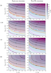 |
Fig. 3 Stability diagrams of Earth-sized tidally locked planets with Earth-like (left panels) and pure CO2 (right panels) atmospheres, and the associated minimum surface temperature. Quantities are plotted as functions of the stellar flux normalised by the Earth’s stellar flux, F⋆/F⊕ (horizontal axis), and the surface pressure, ps, in logarithmic scale (vertical axis). From bottom to top: 0D (1 × 1 grid), 1D (1 × 50 grid), 1.5D (2 × 50 grid), and 2D (32 × 50 grid) instances of the meta-model. Large red dots indicate simulations where the atmosphere remained stable, while small blue dots indicate atmospheric collapse. The dashed orange (or dotted pink) line indicates the collapse pressure pC;low (or pC;up) corresponding to the lower (or upper) bound of the nightside surface temperature predicted by Wordsworth’s analytic model and given by Eq. (11). |
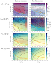 |
Fig. 4 Stability diagrams of Earth-sized tidally locked planets hosting Earth-like (left panels) and pure CO2 (right panels) atmospheres, with turbulent diffusion (TD, four bottom panels) and without turbulent diffusion (NTD, four top panels), superimposed on the maps of various quantities. From bottom to top: day-night advection timescale with turbulent diffusion, day-night advection timescale with turbulent diffusion over the lower bound estimated analytically by Koll & Abbot (2016) using the heat engine theory, ratio of day-night advection timescales with and without turbulent diffusion, and nightside surface temperature difference between the cases with and without turbulent diffusion. The curves and symbols are the same as in Fig. 3. |
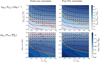 |
Fig. 5 Maximum of Eulerian mean stream function (top) and its ratio over the scaling law (bottom) for Earth-sized planets hosting Earth-like (left panels) and pure CO2 (right panels) atmospheres. The two estimates of the Eulerian mean stream function are given by Eqs. (52) and (53), respectively. The curves and symbols are the same as in Fig. 3. |
6 From slow to fast rotation
Since the GCMM is designed to study the asymptotic regime of slowly rotating planets, where mean flows are predominantly driven by the day-night temperature gradient, we have ignored the effects of rotation on the general circulation until now. As discussed in Sect. 2, the impact of these effects is mainly controlled by the non-dimensional equatorial Rossby deformation radius  introduced in Eq. (1). The zero-spin rate limit treated by the model corresponds to
  . In reality Coriolis acceleration tends to deviate the divergent winds blowing between the sub-stellar and the anti-stellar points. This alters the large-scale circulation regime, which switches from the bi-dimensional Hadley cell described by the 2D model to the 3D structure characterising fast rotators, where super-rotation develops, as
  decays. In this section we investigate the limitations of the bidimensional approach by benchmarking the results obtained with the 2D instance of the GCMM against the simulations performed with the THOR GCM (Mendonça et al. 2016; Deitrick et al. 2020), which solves the 3D non-hydrostatic Euler equations on an icosahedral grid. Particularly, THOR fully accounts for the horizontal vortical component of mean flows that is ignored in the 2D model.
Four simulations were performed with THOR for the pure CO2 atmospheres defined by Table 2. They each correspond to a given spin period Ρ taken in a range spanning from fast to slow rotators all things being equal (P = 10−3, 10−2, 10−1, 100 P0 with P0 = 365 days). For comparison, one additional simulation was run with the 3D GCM in the slow rotator case (P = P0) by assuming no turbulent diffusion or sensible surface-atmosphere heat exchanges. In these simulations, the values of the surface pressure (ps = 0.18 bar) and stellar flux (F⋆ = F⊕) were chosen so that the studied cases are in the vicinity of the threshold between the stability and collapse regions predicted by the 2D instance of the meta-model (see Fig. 3, top right panel). The horizontal resolution of the icosahedral grid used in the model was set to ~4 degrees, and the atmosphere was divided into 40 vertical intervals logarithmically refined in the vicinity of the surface with a top altitude of 37000 m and a 2 m-thick lowest layer. For the sake of consistency, the simulations were run using the double-grey approximation for radiative transfer and a physical setup as close as possible as that implemented in the GCMM. After the circulation and radiative transfer have reached a state of equilibrium, the physical quantities were averaged over the longitude of the TLCs to transform the 3D fields into 2D fields similar to those displayed in Fig. 1. The bulk dimensionless equatorial Rossby deformation length ( ) was computed from the resulting mass-averaged temperature using the expression given by Eq. (4). In parallel of the simulations performed with THOR, a simulation corresponding to the zero-spin rate limit was run with the 2D instance of the meta-model.
Notwithstanding the vertical coordinates used in dynamical cores – altitude-based in THOR, and mass-based in the GCMM – the main differences between the two models essentially lie in the description of the surface thermal response, PBL, and numerical energy dissipation. In THOR, the surface temperature evolution is integrated using a 0D thermodynamic equation parametrised by an effective surface heat capacity ( ), while a ID soil heat transfer scheme is used in the GCMM (see Appendix G). In the treatment of the PBL, the two models closely follow the method proposed by Holtslag & Boville (1993), except for some parameters, which are set to different values. For instance, the asymptotic length scale characterising the evolution of the mixing length with altitude (Eq. (31)) for the heat equation is set to three times the function used for the momentum equation (Eq. (F.6)) in THOR, while the same function is used in both cases in the GCMM. As regards numerical energy dissipation, all THOR simulations utilised fourth-order horizontal hyper-diffusion and 3D divergence damping with a non-dimensional coefficient Dhyp = Ddiv = 0.002 (Mendonça et al. 2016; Deitrick et al. 2020, for descriptions of the hyper-diffusion scheme). We additionally used sixth-order vertical hyper-diffusion with a non-dimensional coefficient of Dver = 5 × 10⁻⁴. Finally, a sponge layer was applied to the upper 25% of the model domain to damp spuriously reflected waves off the top boundary, with a damping timescale of 5000 s (see Mendonça et al. 2018; Deitrick et al. 2020, for the sponge layer description).
Figure 6 shows the simulation results. The dayside and nightside surface temperatures, as well as the day night surface temperature difference, are plotted as a function of the bulk equatorial Rossby deformation radius (top panels). Solid lines designate the temperatures obtained in TH0R 3D simulations, and the horizontal dashed lines the temperatures obtained in the 2D simulation performed with the meta-model. The dotted lines indicate the corresponding averaged dayside and nightside surface temperatures predicted by Wordsworth’s purely radiative greenhouse model (Wordsworth 2015). The temperatures obtained from the 3D simulation performed in the absence of turbulent diffusion are designated by the star symbol ⋆ In addition, the Eulerian mean stream function defined in Eq. (51) is plotted for the 2D model and the two extrema of the 3D model (P = 365 days and P = 0.365 days) as functions of pressure (or sigma coordinate) and the latitude of the TLCs, where the north and south poles correspond to the sub-stellar and anti-stellar points, respectively (bottom panels).
We first consider the evolution of surface temperatures with  (Fig. 6, top panels). Whereas the dayside surface temperature predicted by 3D GCM simulations is hardly affected by the planet’s rotation, the nightside surface temperature increases monotonically with the equatorial Rossby deformation radius until it converges towards the asymptotic limit of slow rotators described by the 2D model. The effect of rotation is particularly significant for the minimum surface temperature, which varies by ~35 K between the two extremal cases. This difference results from the decay of day night advection provoked by the breaking of the day night overturning circulation in the fast rotator regime (
 ). The super-rotating equatorial jets induced by Coriolis effects do not compensate the overturning circulation in terms of mass flux crossing the terminator annulus, which makes the nightside surface temperature decrease. However, we remark that the nightside temperature stays close from the asymptotic limit of slow rotators from the moment that
  , the difference of the cases P = 36.5 days and P = 365 days to this limit being less than 3 K. This suggests that the 2D model is relevant to describe the climate and large-scale circulation regime of the planet for equatorial Rossby deformation radii exceeding the critical value
  . Below this value, the circulation and heat redistribution are strongly affected by the planet’s rotation.
Additionally, we remark that the 2D model and the THOR GCM are in agreement with each other for the nightside surface temperature, which is greater by ~2 K only in 3D simulations. The discrepancy between the two models is more significant for the dayside average temperature, where the effects of the PBL in surface-atmosphere heat exchanges are predominant. As observed in the 2D model, the frictional interaction of mean flows with the planet’s surface taking place in the PBL tends to increase the atmospheric stability against collapse by warming up the nightside surface hemisphere. To understand whether the differences in PBL parameters between the 2D and 3D models could be the source of the discrepant dayside temperatures, one additional THOR simulation was run at the slowest rotation rate. In this simulation, the asymptotic scale lengths (for heat and momentum mixing in the boundary layer) were set equal to those used in the 2D model. The resulting values are shown as the square points in top panels of Fig. 6. Interestingly, these results are nearly indistinguishable from the simulation with different scale lengths used for the heat and momentum equations, indicating that the scenario is insensitive to the asymptotic scale lengths used in Eq. (31).
We now consider the snapshots of the Eulerian mean stream function (Fig. 6, bottom panels). We remark that the vertical coordinates used for the plots in the 2D and 3D cases differ from each other, which leads to slight distortions of the distributions. The sigma coordinate is such that σ = 1 everywhere at planet’s surface, while the surface pressure is less than the globally averaged surface pressure on the dayside, and greater on the nightside due to the day night thermal forcing gradient. As a consequence, isobars in sigma coordinates are slightly shifted downwards on the dayside and upwards on the nightside. The 3D simulation performed with THOR GCM in the slow rotation regime is in good agreement with the 2D simulation performed with the GCMM in the zero-spin rate limit (Fig. 6, bottom left and middle panels). The two snapshots both exhibit large day-night cells of comparable strengths, albeit slightly weaker in the 2D model. The snapshot corresponding to the fast rotation regime (bottom right panel) exhibits more complex features due to Coriolis effects although a weak day night cell still remains visible.
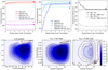 |
Fig. 6 Dayside and nightside surface temperatures vs. normalised equatorial Rossby deformation radius |

7 Concluding remarks
In this work we have developed a GCMM to bridge the gap between the analytic solutions provided by simplified greenhouse models for synchronous planets and the numerical simulations obtained from 3D GCMs in the asymptotic regime of slow rotators. This model hierarchy is based on a systematic bottom up approach in the spirit of Held (2005), wherein the number of degrees of freedom determines the key sources of complexity that are added or subtracted. The solver of the GCMM integrates the HPEs using the finite-volume method for arbitrary numbers of horizontal and vertical intervals, each configuration being an instance of the meta-model. Consistent with a previous analytical study (Auclair-Desrotour & Heng 2020), the physics implemented in the meta-model includes double-grey radiative transfer, turbulent diffusion in the PBL, and soil heat conduction. Particularly, the meta-model was designed so that the solutions obtained with the 0D instance exactly correspond to the analytic solutions of the purely radiative box model detailed in Sect. 3.3 of Auclair-Desrotour & Heng (2020).
As a first step, we proceeded to a vertical model inter-comparison by running grid simulations for four instances of the meta-model (0D, 1D, 1.5D, and 2D) in the cases of dry Earthlike and pure CO2 atmospheres. In each case, we computed from simulations the nightside surface temperature of the planet as a function of the stellar flux and surface pressure as well as the resulting stability diagrams of the atmosphere against collapse. These diagrams were compared to the scaling laws predicted by the analytic theory. With the 0D and 1D instances of the meta-model, we recovered the stability diagrams predicted by simplified radiative models in the optically thin regime, which shows that the globally isothermal approximation used in these models is relevant in this regime. The 1.5D instance tends to underestimate the atmospheric stability, by predicting a collapse pressure 25% to 80% larger than that given by radiative box models. Conversely, the collapse pressure computed using the 2D instance of the meta-model is 10% to 40% smaller than the analytic estimate owing to the warming effect of the PBL, which is less than the theoretical 75% maximum decrease predicted by radiative models, albeit still significant.
As a second step, we investigated the role played by the PBL in the thermal state of equilibrium and atmospheric circulation of the planet by examining with the 2D instance of the GCMM how the turbulent diffusion taking place in the PBL alters the nightside temperature, the day night advection timescale, and the collapse pressure. We compared the advection timescale obtained from simulations with the analytic scaling law proposed by Koll & Abbot (2016). We observed that the turbulent diffusion taking place in the PBL increases the nightside surface temperature by 4–14 K around the threshold of the stability region. However, we found that the PBL can also contribute to cooling the nightside surface of the planet by acting on the day night advection timescale in the transition zone between optically thin and optically thick atmospheres. This result was corroborated a posteriori by 3D GCM simulations. The effect of the PBL on the large-scale circulation is complex and depends on the interplay between the advection and radiative timescales. The day night advection timescale estimated with the 2D model varies over two orders of magnitude in the studied domain of stellar fluxes and surface pressures, with values ranging between 8 and 500 days. In the optically thin regime its evolution matches the scaling law derived by Koll & Abbot (2016) relatively well, but it diverges from it at high pressures and low stellar fluxes. We noticed that this behaviour also depends on the thermodynamic and absorption properties of the atmosphere in the optically thick regime. In addition we empirically obtained, for the circulation of slowly rotating rocky planets, a scaling law analogous to that established analytically by Innes & Pierrehumbert (2022) for sub Neptunes.
As a third and final step, we characterised the limitations of the slow rotator approximation that forms the foundations of the meta-model by performing simulations with the THOR 3D GCM, which fully accounts for the effects of rotation on mean flows. We computed from these simulations the evolution of the planet’s dayside and nightside surface temperatures as functions of the dimensionless equatorial Rossby deformation radius, which controls the large-scale circulation regime of the planet. The results obtained with the 3D GCM were compared with the outcomes of the 2D instance of the meta-model. The 3D GCM simulations highlight the transition between the slow and fast rotation regimes. We found that the 2D model properly accounts for the climate and large scale atmospheric circulation from the moment that the normalised equatorial Rossby deformation radius is greater than the critical value  , which corresponds to a broad region of the parameter space. In the slow rotation regime, the circulation and surface temperature predicted by the THOR 3D GCM and the 2D instance of the meta-model are similar.
This study is a first attempt to fill the continuum between analytic greenhouse models and 3D GCMs in a self-consistent way. The obtained results show that the meta-modelling approach is efficient at disentangling the mechanisms that determine the climatic state of the planet, which are narrowly coupled together in GCMs. This approach allows models of various complexities, albeit with the very same physical setup, to be run in parallel series so that each simulation can be interpreted using the others. As a consequence, the final outcome of the meta-model conveys information not only on the climate itself but also on the separated contributions of key physical ingredients such as radiative transfer, atmospheric structure, dynamics, and turbulent friction in the PBL. In addition to these diagnostic aspects, the meta-modelling approach appears as a robust method for refining the analytic theory of planetary climates given that it allows the relevance of solutions obtained at low spatial dimensionality to be assessed with consistently generated GCM numerical solutions. Finally, we note that the meta-modelling approach can be extended to moist atmospheres and rapidly rotating planets, but we leave that to the content of a future study.
Acknowledgements
The authors thank the anonymous referee for helpful comments that improved the manuscript, and Vera Matarese for inspiring discussions about the representational capacity of numerical simulations. They acknowledge financial support from the European Research Council via the Consolidator grant EXOKLEIN (grant number 771620). Kevin Heng also acknowledges partial financial support from the National Swiss Foundation, the PlanetS National Center of Competence in Research, the Center for Space & Habitability and the MERAC Foundation. This research has made use of NASA’s Astrophysics Data System. The authors gratefully acknowledge the open source softwares that made this work possible: numpy (Harris et al. 2020), matplotlib (Hunter 2007), scipy (Virtanen et al. 2020). THOR calculations were performed on UBELIX (http://www.id.unibe.ch/hpc), the HPC cluster at the University of Bern.
Appendix A Non-dimensional primitive equations
The model solves the HPEs given by Eqs. (15-18) in their non-dimensional form. Although it is not used in the present study, the moisture conservation equation is included in the solver and we give it here for the sake of generality. In its conservative form, this equation reads (e.g. Yao & Stone 1987)
 (A.1)
(A.1)
where q designates the specific humidity of any tracer, and  the corresponding net evaporation or condensation rate per unit mass. Since the elemental unit of time of the discretised equations is the dynamical time step Δt used in the time-differencing scheme, it is convenient to normalise the time by Δt so that the time lapse between two dynamical time steps is always unity.
We then introduce the reference pressure p0, temperature T0, and specific humidity qo, from which we can define the reference velocity υ0, energy per unit mass e0, density p0, force per unit mass F0, heat power per unit mass Q0, net evaporation per unit mass  , Exner function E0, and potential temperature Θ0,
 (A.2)
(A.2)
Besides, we make the horizontal coordinate vary within the range [0,1] like the vertical coordinate by re-normalising the colatitude (θ). The normalised variables and colatitude are therefore defined as
 (A.3)
(A.3)
As a second step, the spatial coordinates ( ) are converted to grid coordinates4, (Y, Z). In this transformation, the normalised colatitude
  and vertical coordinate σ = σ (Ζ) are assumed to be monotonie functions of Y and Z, respectively. These functions are defined further so that the interval between the two boundaries of a finite volume is equal to 1 both in the horizontal and in the vertical directions, as showed by Fig. A.1. The transformation (
 ) is defined at any point by the horizontal and vertical metric coefficients, CY and Cz, defined as
 (A.4)
(A.4)
which yields the change relations of partial derivatives
 (A.5)
(A.5)
 (A.6)
(A.6)
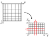 |
Fig. A.1 Change of coordinate, ( |

We remark that the change of coordinate is just a dilation if the adopted horizontal and vertical spacings are uniform since cY and cZ are constants in this case. We also notice that cz < 0 with the chosen sigma coordinate given that σ decreases monotonically as the altitude increases.
To include the metric in the primitive equations, we introduce the respective covariant and contravariant horizontal velocities,
 (A.7)
(A.7)
the normalised area density (area per unit length),
 (A.8)
(A.8)
mass density5,
 (A.9)
(A.9)
and horizontal and vertical mass flux densities,
 (A.10)
After the above manipulations, the system of HPEs given by Eqs. (15-18) and Eq. (A.1) become the normalised primitive equations
 (A.11)
 (A.12)
 (A.13)
 (A.14)
 (A.15)
where the normalised Exner function, derived from Eq. (20), is expressed as a function of the normalised pressure  ,
,
 (A.16)
As may be noticed, with the normalisation adopted in Eq. (A.3), the dynamics of the non-dimensional HPEs is controlled by one unique dimensionless parameter,
 (A.17)
which is a global Courant number weighting the contribution of horizontal advection6. The density is not a variable of the primitive equations but can be evaluated using the perfect gas equation,
 (A.18)
while the vertical velocity can be calculated from the conversion formula
![${\upsilon _z} = {{{\upsilon _z}0} \over {\tilde m}}\left[ {\tilde m{{\partial \tilde \phi } \over {\partial \tilde t}} + bV{{\partial \tilde \phi } \over {\partial Y}} + W{{\partial \tilde \phi } \over {\partial Z}}} \right],$](/articles/aa/full_html/2022/07/aa43099-22/aa43099-22-eq122.png) (A.19)
(A.19)
where we have introduced the characteristic vertical velocity
 (A.20)
Appendix B Dynamical core
The system of prognostic equations given by Eqs. (A.11-A.15) is integrated numerically using a standard finite-volume method. This appendix details the main features of the dynamical core of our model.
Appendix B.1 Grid
The primitive equations are discretised and solved on a staggered Arakawa C grid (Arakawa & Lamb 1977). The atmosphere is divided into elemental cells. Mass fluxes and velocities are evaluated at cell interfaces, and volume quantities ( ) at cells centres, except the pressure, which is evaluated at horizontal cells interfaces. A diagram representing the grid is shown by Fig. B.1.
As a first step, the spatial domain defined by (![$\left( {\widetilde \theta ,\sigma } \right) \in {\left[ {0,1} \right]^2}$](/articles/aa/full_html/2022/07/aa43099-22/aa43099-22-eq125.png) ) is divided into non-uniform intervals both along the horizontal and vertical directions. There are M intervals for the colatitude, and N intervals for the vertical coordinate, which represents M × N cells. The vertical spacing can be specified arbitrarily. It determines the coordinates of cell boundaries. We note that the σ levels of cell centres can be explicitly computed from the σ levels of cell boundaries if pt = 0 (standard sigma coordinate) as discussed in Sect. B.2.
) is divided into non-uniform intervals both along the horizontal and vertical directions. There are M intervals for the colatitude, and N intervals for the vertical coordinate, which represents M × N cells. The vertical spacing can be specified arbitrarily. It determines the coordinates of cell boundaries. We note that the σ levels of cell centres can be explicitly computed from the σ levels of cell boundaries if pt = 0 (standard sigma coordinate) as discussed in Sect. B.2.
As as second step, the change of coordinates (![$\left( {\widetilde \theta ,\sigma } \right) \to \left( {Y,Z} \right) \in \left[ {0,M} \right] \times \left[ {0,N} \right]$](/articles/aa/full_html/2022/07/aa43099-22/aa43099-22-eq126.png) ) is applied, and the corresponding metric coefficients cY and cZ are calculated. Typically, for a uniform grid,
) is applied, and the corresponding metric coefficients cY and cZ are calculated. Typically, for a uniform grid,  , and thus cY = 1/M everywhere. The case of non-uniform horizontal intervals is more complicated, since this implies
  -dependent coefficients. To treat the general case, we adapt the method employed for the horizontal grid in the LMDZ GCM to the 1D case: each surface area is divided into two subsurface areas, as shown by Fig. B.2, and the CY are evaluated at subarea centres and boundaries (Sadourny 1975a,b). The cZ are just the difference between two vertical levels. We introduce the difference and average operators,
 (B.1)
(B.1)
![${\overline \psi ^X}\left( X \right) = {1 \over 2}\left[ {\psi \left( {X + {1 \over 2}} \right) + \psi \left( {X - {1 \over 2}} \right)} \right],$](/articles/aa/full_html/2022/07/aa43099-22/aa43099-22-eq130.png) (B.2)
(B.2)
where X is a placeholder for Y or Z and ψ any variable. In this formalism, the cZ are simply expressed as  .
.
In the present work, we use a vertical grid refined near the surface and the upper boundary. The sigma coordinates of vertical levels are given by the function
![$\sigma \left( x \right) = {1 \over 2}\left[ {1 + \cos \left( {\pi {x^a}} \right)} \right],$](/articles/aa/full_html/2022/07/aa43099-22/aa43099-22-eq132.png) (B.3)
(B.3)
where x ≡ Z/N takes its values between 0 and 1. Here, the exponent a is a dilation coefficient that controls the growth or decay rate of vertical intervals in the vicinity of the lower and upper bounds. Introducing the vertical coordinate difference between the lowest model level and the surface, ∆σSL:, this parameter is defined as
 (B.4)
(B.4)
For an isothermal temperature profile near planet’s surface,  , where H is the local pressure height. In practice, we set
  .
.
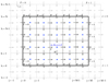 |
Fig. B.1 Staggered grid. In the adopted finite-volume method, the horizontal axis is divided into M intervals and the vertical axis into N intervals, which represents M × N cells (here, M = 5 and N = 4). Horizontal levels are indexed by j and vertical levels by k. The left and right boundaries of the physical domain correspond to |


Appendix B.2 Exner Function
The calculation of the Exner function follows the method described by Arakawa & Lamb (1977) and Hourdin (1994), which is summarised here. Instead of computing E at the middle of the layer by extrapolating the pressure at the middle of the layer from the level pressures at the interfaces, which is computationally expensive, one rather uses a supplementary relationship between the interface levels and the Exner function. This relationship is directly derived from considerations about energy conservation principles within the atmospheric air column. Particularly, in the hydrostatic approximation, the internal and potential energy are proportional, which implies (Arakawa & Lamb 1977); Hourdin 1994)
 (B.5)
(B.5)
where m = pdz is the infinitesimal parcel of mass per unit surface, and mcol the mass of the air column per unit surface. The expression of ф as a function of Θ and E is simply obtained by making use of the hydrostatic balance equation given, in grid vertical coordinates, by
 (B.6)
(B.6)

which allows us, noticing that RdT = κΘΕ, to rewrite Eq. (B.5) as
![$\int_0^{{m_{{\rm{col}}}}} {\left[ {\int_0^Z {\Theta {{\partial E} \over {\partial Z'}}dZ'} + k\Theta E} \right]} \,\,{\rm{d}}m = 0.$](/articles/aa/full_html/2022/07/aa43099-22/aa43099-22-eq141.png) (B.8)
(B.8)
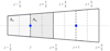 |
Fig. B.2 Subdivision of a surface area into two subsurface areas, A1 and A2 (light grey and grey regions). The big blue dots indicate the centres of horizontal intervals. The areas are calculated analytically by taking their dependence on colatitude into account. The configuration of the diagram corresponds to small horizontal intervals, where this dependence is approximately linear. |
The discretised form of the first term is given by
 (B.9)
(B.9)
where Θl, El are the potential temperature and Exner function evaluated at the middle of the layer, indexed by l = 0, . . . , N − 1 (for N vertical intervals), and Es = Cp (p/pref)κ is the Exner function evaluated at the planet’s surface. By making use of the difference and average operators introduced in Eqs. (B.1) and (B.2), the preceding equation can be rewritten in the compact form
![$\int_0^{{Z_l}} {{\rm{\Theta }}{{\partial E} \over {\partial Z}}{\rm{d}}Z' = {{\sum\limits_{l = 0}^{N - 1} {\left[ {{{\overline {\rm{\Theta }} }^Z}{\delta _Z}E} \right]} }_k},} $](/articles/aa/full_html/2022/07/aa43099-22/aa43099-22-eq143.png) (B.10)
(B.10)
![$\matrix{{{{\left[ {{{{\rm{\bar \Theta }}}^Z}{\delta _Z}E} \right]}_k}} \hfill & { = \left( {{{{{\rm{\Theta }}_k} + {{\rm{\Theta }}_{k - 1}}} \over 2}} \right)\left( {{E_k} - {E_{k - 1}}} \right),} \hfill & {k = 1, \ldots ,N - 1,} \hfill \cr {{{\left[ {{{{\rm{\bar \Theta }}}^Z}{\delta _Z}E} \right]}_0}} \hfill & { = {{\rm{\Theta }}_0}\left( {{E_0} - {E_s}} \right).} \hfill & {} \hfill \cr } $](/articles/aa/full_html/2022/07/aa43099-22/aa43099-22-eq144.png)
Then, introducing the mass ml per unit area of layer l and interchanging the sums in the double integral, we obtain
![$\sum\limits_{l = 0}^{N - 1} {{m_l}\int_0^{{Z_l}} {{\rm{\Theta }}{{\partial E} \over {\partial Z}}{\rm{d}}Z' = \sum\limits_{l = 0}^{N - 1} {{m_l}{{\sum\limits_{k = 0}^l {\left[ {{{\overline {\rm{\Theta }} }^Z}{\delta _Z}E} \right]} }_k},} } } $](/articles/aa/full_html/2022/07/aa43099-22/aa43099-22-eq145.png) (B.12)
(B.12)
![$ = \sum\limits_{k = 0}^{N - 1} {{{\left[ {{{\overline {\rm{\Theta }} }^Z}{\delta _Z}E} \right]}_k}\sum\limits_{l = k}^{N - 1} {{m_l}.} } $](/articles/aa/full_html/2022/07/aa43099-22/aa43099-22-eq146.png) (B.13)
(B.13)
In the above equation, we recognise the atmospheric mass per unit surface above the k interfaces (k = 0‚…, N), which is expressed in the framework of the hydrostatic approximation as
 (B.14)
![$\sum\limits_{l = 0}^{N - 1} {{m_l}} \int_0^{{Z_l}} {{\rm{\Theta }}{{\partial E} \over {\partial Z}}dZ' = {1 \over g}\sum\limits_{k = 0}^{N - 1} {{{\left[ {{{\overline {\rm{\Theta }} }^Z}{\delta _Z}E} \right]}_k}{p_k}.} } $](/articles/aa/full_html/2022/07/aa43099-22/aa43099-22-eq148.png)
Finally, expanding the coefficients of the sum, we remark that this later may be rewritten
![${\sum\limits_{k = 0}^{N - 1} {\left[ {{{\overline {\rm{\Theta }} }^Z}{\delta _Z}E} \right]} _k}{p_k} = \sum\limits_{k = 0}^{N - 1} {{{\rm{\Theta }}_k}{{\left[ {{{\overline {p{\delta _Z}E} }^Z}} \right]}_k},} $](/articles/aa/full_html/2022/07/aa43099-22/aa43099-22-eq149.png) (B.16)
(B.16)
with the conventions
![${\left[ {{{\overline {p{\delta _Z}E} }^Z}} \right]_0} = {1 \over 2}\left( {{E_1} - {E_0}} \right){p_1} + \left( {{E_0} - {E_{\rm{s}}}} \right){p_0}$](/articles/aa/full_html/2022/07/aa43099-22/aa43099-22-eq150.png) (B.17)
(B.17)
![${\left[ {{{\overline {p{\delta _Z}E} }^Z}} \right]_{N - 1}} = {1 \over 2}\left( {{E_{N - 1}} + {E_{N - 2}}} \right){p_{N - 1}} + \left( {{E_t} - {E_{N - 1}}} \right){p_t}.$](/articles/aa/full_html/2022/07/aa43099-22/aa43099-22-eq151.png) (B.18)
(B.18)
Thus, in the general case, the Exner function can be evaluated at cell centres by applying, at all vertical levels, the relation
 (B.19)
The use of standard sigma coordinates appreciably reduces the complexity of the problem. Assuming pt = 0 and introducing the notation s = σκ, the preceding equation simplifies to
 (B.20)
which allows the sigma coordinates of cell centre levels to be pre-calculated. Indexing these levels by k = o, …,N – 1 and the intermediate (or interface) σ levels by k = o,…, N , we have
![$\matrix{{{{\left[ {{{\overline {\sigma {\delta _Z}s} }^Z}} \right]}_k}} \hfill & { = \kappa {s_k}{{\left[ {{\delta _Z}\sigma } \right]}_k}\,for\,k = 1, \ldots ,N - 2,} \hfill \cr {{{\left[ {{{\overline {\sigma {\delta _Z}s} }^Z}} \right]}_0}} \hfill & { = {1 \over 2}\left( {{s_1} - {s_0}} \right){\sigma _1} + \left( {{s_0} - {s_{\rm{s}}}} \right){\sigma _0} = \kappa {s_0}\left( {{\sigma _1} - {\sigma _0}} \right),} \hfill \cr {{{\left[ {{{\overline {\sigma {\delta _Z}s} }^Z}} \right]}_{N - 1}}} \hfill & { = {1 \over 2}\left( {{s_{N - 1}} - {s_{N - 2}}} \right){\sigma _{N - 1}} = \kappa {s_{N - 1}}\left( {{\sigma _N} - {\sigma _{N - 1}}} \right)} \hfill \cr } $](/articles/aa/full_html/2022/07/aa43099-22/aa43099-22-eq154.png) (B.21)
(B.21)
where ss = 1 and st = 0 are the value of s at planet’s surface and atmospheric upper boundary, respectively.
In practice, the Exner function is evaluated at grid centre levels by solving an algebraic equation of the form AX = B. In the case of standard sigma coordinates (pt = 0), this calculation is performed only once, when the grid is constructed. The algebraic system to solve then writes
![$\left[ {\matrix{{{A_{0,0}}} & {{A_{0,1}}} & {} & {} & {} \cr {{A_{1,0}}} & {{A_{1,1}}} & {{A_{1,2}}} & {} & {} \cr {} & {{A_{k,k - 1}}} & {{A_{k,k}}} & {{A_{k,k + 1}}} & {} \cr {} & {} & {{A_{N - 2,N - 3}}} & {{A_{N - 2,N - 2}}} & {{A_{N - 2,N - 1}}} \cr {} & {} & {} & {{A_{N - 1,N - 2}}} & {{A_{N - 1,N - 1}}} \cr } } \right]\left[ {\matrix{{{s_0}} \cr {{s_1}} \cr {{s_k}} \cr {{s_{N - 2}}} \cr {{s_{N - 1}}} \cr } } \right] = \left[ {\matrix{ {{B_0}} \cr {{B_1}} \cr {{B_k}} \cr {{B_{N - 2}}} \cr {{B_{N - 1}}} \cr } } \right],$](/articles/aa/full_html/2022/07/aa43099-22/aa43099-22-eq155.png) (B.22)
(B.22)
where the sk is the coordinate s = σκ evaluated at the mid-level of the k-layer, A the tri-diagonal matrix of coefficients
 (B.23)
 (B.24)
 (B.25)
 (B.26)
and B the vector of coefficients
 (B.27)
 (B.28)
 (B.29)
In these equations, ss = 1 and st = o are the values of s at planet’s surface and atmospheric top, respectively. This procedure can be applied from the moment that Ν > 1. If there is only one layer, then the mid-level coordinate of the unique layer is set to 
Appendix B.3 Discretisation of the Primitive Equations
The normalised prognostic equations given by Eqs. (A.11-A.15) are discretised by making use of the difference and average operators defined by Eqs. (B.1) and (B.2), and become
 (B.30)
![$\matrix{ {{\partial \over {\partial \tilde t}}\left( {{{\overline {\tilde m} }^Y}{{\tilde \upsilon }_\theta }} \right) + b{\delta _Y}\left( {{{\overline V }^Y}{{\overline {{{\tilde \upsilon }_\theta }} }^Y}} \right) + {\delta _Z}\left( {{{\overline {\rm{W}} }^Y}{{\overline {{{\tilde \upsilon }_\theta }} }^Z}} \right)} \hfill \cr {\;\;\;\;\;\;\;\;\;\;\;\;\;\; + {b \over {{c_Y}}}\left[ {{{\overline {\tilde m} }^Y}{\delta _Y}\tilde \phi + {{\overline {\tilde m\tilde \Theta } }^Y}\left( {{\delta _Y}\tilde E} \right)} \right] = {{\overline {\tilde m} }^Y}{{\tilde F}_\theta },} \hfill \cr } $](/articles/aa/full_html/2022/07/aa43099-22/aa43099-22-eq165.png) (B.31)
(B.31)
 (B.32)
 (B.33)
 (B.34)
In the right-hand members of these equations, the horizontal force is specified at horizontal interface levels, where the horizontal mass fluxes and velocities are also evaluated, and  and
and  at cell centres. The vertical velocity can be calculated afterwards, when it is necessary, using the formula
![${\upsilon _z} = {{{\upsilon _{z0}}} \over {{{\overline {\tilde m} }^Z}}}\left[ {{{\overline {\tilde m{{\partial \tilde \phi } \over {\partial \tilde t}}} }^Z} + b{{\overline {{{\overline {{\rm{V}}{\delta _Y}\tilde \phi } }^Y}} }^Z} + {\rm{W}}{\delta _Z}\tilde \phi } \right].$](/articles/aa/full_html/2022/07/aa43099-22/aa43099-22-eq171.png) (B.35)
(B.35)
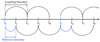 |
Fig. B.3 Time-differencing scheme implemented in the solver. The scheme is based on a leapfrog time step (e.g. Sect. 5.5.2 of Lauritzen et al. 2011), which is replaced by a Matsuno time step (Matsuno 1966a) every nMT = 5 steps. |
Appendix B.4 Time-Differencing Scheme
Following the method used in many GCMs (Hansen et al. 1983; Yao & Stone 1987; Hourdin et al. 2006), the temporal integration of the primitive equations is based on the so-called leapfrog scheme, which is a centred explicit scheme (e.g. Press et al. 2007). Since the leapfrog scheme tends to generate a spurious growth of numerical instabilities over time (e.g. Lauritzen et al. 2011, Sect. 5.5), a Matsuno time step (Matsuno 1966a) is introduced every nMT steps (with nMT = 5) to stabilise the integration, as illustrated by Fig. B.3. Mathematically, denoting the time derivative operator by M, any dynamical variable by ψ, and indexing time steps by n, a leapfrog step is expressed as
 (Β.36)
while a Matsuno step (Matsuno 1966a) consists in the succession of two steps,
 (B.37)
 (Β.38)
where the superscript * is used to designate the intermediate virtual time step. In Fig. B.3, the leapfrog time step is used to compute variables at all dates except t0 and t5, where it is replaced by a Matsuno step. Sink terms associated with numerical dissipation (hyper-diffusion, sponge layer, etc.) are evaluated periodically every nMT dynamical time step, before Matsuno time steps. Physical tendencies are computed every nP dynamical time step (with np = 10).
Appendix C Numerical dissipation
Appendix C.1 Horizontal Hyper-Diffusion
To dissipate energy at grid scale, we introduce a bi-harmonic diffusion (Lauritzen et al. 2011), which is a fourth-order diffusion. This is obtained by applying twice the Laplacian operator to the temperature and horizontal velocity. For any scalar quantity ψ, the horizontal Laplacian operator reads, in our 2D system of coordinates,
 (C.1)
(C.1)
In grid coordinates, it is expressed as
 (C.2)
(C.2)
where  designates the normalised horizontal Laplacian operator,
 (C.3)
(C.3)
We introduce the hyper-Laplacian operator, which is the Laplacian of order q, defined as  . Basically, for the fourth-order hyper-diffusion, q = 2, and
  . In the general case, the 2q-order hyper-diffusion term of any variable ψ is defined by
 (C.4)
(C.4)
where K2q is the hyper-diffusivity. This parameter can be written as a function of the diffusion timescale tdiff and mean horizontal grid spacing  (Lauritzen et al. 2011, Sect. 13.3),
 (C.5)
(C.5)
The normalised hyper-diffusivity  is thus given by
 (C.6)
(C.6)
In order to adapt the hyper-diffusivity to the horizontal grid resolution, it is convenient to introduce the non-dimensional diffusion parameter (Tomita & Satoh 2004); Mendonça et al. 2016)
 (C.7)
(C.7)
which allows us to rewrite diffusivity parameters as
 (C.8)
(C.8)
Bi-harmonic diffusion is used in the model, with a diffusion parameter set to  in agreement with the order of magnitude of commonly used values (Lauritzen et al. 2011, Sect. 13.3).
In the finite-volume approach, hyper-diffusion can lead to numerical instabilities near the poles because of the singularity  of the Laplacian operator. Typically, assuming that ψ is an oscillatory function of the form
  yields
![$\nabla _\sigma ^2\psi = {{{{\left( {n\pi } \right)}^2}} \over {\sin \theta }}\left[ {{{\left( {n\pi } \right)}^{ - 1}}\cos \left( \theta \right)\cos \left( {n\pi \theta } \right) - \sin \left( \theta \right)\sin \left( {n\pi \theta } \right)} \right],$](/articles/aa/full_html/2022/07/aa43099-22/aa43099-22-eq191.png) (C.9)
(C.9)
and thus  in polar regions. To remediate to this problem, it is often chosen to compensate the singularity introduced by the Laplacian by annihilating the diffusivity parameter at the poles (Lauritzen et al. 2011, Sect. 13.3). Basically, the isotropic diffusivity introduced in Eq. (C.4) is multiplied by
  , where α is a coefficient of anisotropy
  typically). This anisotropic diffusion solves the stability problem but can also induce unphysical boundary effects near the poles. Following Majewski et al. (2002), we apply a bi-harmonic diffusion (q = 2) to the temperature and horizontal velocity υӨ. We use the same diffusion coefficient for both terms. Thus,
 (C.1O)
 (C.11)
In addition, we apply to the top layer of the model an harmonic diffusion of the form
 (C.12)
 (C.13)
In order to verify that the mean flow and temperature distribution are insentitive to the hyper-diffusion scheme, simulations were run for various values of the non-dimensional diffusion parameter y introduced in Eq. (C.7), namely γ = 10−5, 10−4, 10−3. These validation tests were performed for the Earth-like case of Table 2 with the same surface pressure and stellar flux as in Fig. 1. Figure C.1 shows the two-day averaged temperature snapshots obtained for each value of γ, as well as the associated mean flows. We observe that varying the value of γ over two orders of magnitude hardly alters the temperatures and wind speeds. The minimum nightside temperature after convergence is Tη = 231.5 Κ, Tn =231.7 K, and Ta = 231.8 K, for γ = 10−5, 10−4, 10−3, respectively. Similarly, the maximum wind speed varies between 59.55 m s−1 and 62.08 m s−1 (see Fig. C.1). These variations correspond to a 0.1% difference for the minimum surface temperature, and to a 4.2% difference for the maximum wind speed. Winds are thus more sensitive to the hyper-diffusion scheme than the nightside surface temperature, although the observed dependence is relatively weak in both cases. Nevertheless, this dependence is expected to be more important for extreme values of γ because such values would lead either to under-dissipated or to over-dissipated flow fields, as shown by Thrastarson & Cho (2011). Typically, with a value of γ smaller than the adopted one by several orders of magnitude, the flow rapidly becomes numerically unstable at grid scale, which induces spurious fluctuations and may cause the run to abort.
 |
Fig. C.1 Two-day averaged temperature snapshots for various values of the hyper-diffusion parameter (see Eq. (C.7)). Left: γ = 10−5. Middle: γ = 10−4. Right: γ = 10−3. Simulations were performed for the Earth-like case of Table 2 with a stellar irradiation of 1366 W m−2 and a 1 bar surface pressure, similar to as in Fig. 1. |
Appendix C.2 Sponge Layer
In extreme cases (low surface pressure and high stellar flux), the strong thermal forcing of the atmosphere on the dayside generates instabilities that can lead to negative pressures near the top of the model. Particularly, it generates internal gravity waves that propagate upwards with amplitudes becoming very large as the atmospheric density tends to zero7. These waves are reflected downwards by the upper boundary, which acts as a wall (no vertical mass flow). Owing to the weak density, such extreme fluctuations have dramatic repercussions on the computation of mass flows and are thereby a source of unphysical values that make runs abort. Thus, in addition with the hyper-diffusion scheme, the use of a sponge layer is necessary in cases where the surface pressure is low and the stellar irradiation is strong.
The sponge layer is a numerical dissipation process that strongly damps wind flows diverging from a prescribed equilibrium profile in the upper regions of the atmosphere, with an efficiency increasing with the altitude. In the present model, we use a Rayleigh friction sponge, which is based on a linear relaxation term of generic form (e.g. Lauritzen et al. 2011, Sect. 13.4)
 (C.14)
where kSL designates the Rayleigh damping coefficient of the sponge layer and  the equilibrium velocity profile near the upper boundary. This profile is set to the standard value
  . Following Polvani & Kushner (2002), we opt for a vertical profile of the Rayleigh coefficient of the form
 (C.15)
In the above piecewise function, σSL corresponds to the critical normalised pressure below which the sponge layer is applied while kSL;max is the maximum value of the Rayleigh friction coefficient. This parameter has dimensions of a frequency and is the inverse of the minimum damping timescale of the sponge layer tSL;min The smaller tSL;min, the stronger the damping in the sponge layer. In the model, the maximum Rayleigh coefficient is set to kSL;max = 0.5 day−1, while the thickness of the sponge layer is defined as a function of the stellar flux and surface pressure.
Appendix D Convective adjustment scheme
The turbulent diffusion scheme implemented described by Sect. 3.3 is not sophisticated enough to prevent super-adiabatic vertical temperature gradients,
 (D.1)
(D.1)
If such an unstable profile is produced by the model, it may generate numerical errors in the solution and lead the run to crash. In order to prevent this behaviour, a convective adjustment scheme can be activated in simulations. This scheme tends to regularise the potential temperature profile every physical timestep by correcting the tendencies in heat fluxes while conserving the entropy over the air column. The convective adjustment scheme used in the present work is similar to that implemented in the LMDZ and THOR GCMs (Hourdin et al. 1993; Mendonça & Buchhave 2020).
 |
Fig. D.1 Construction of the stable temperature profile in the convective adjustment scheme. An initially unstable region of the air column spreading from layer l1 to layer l2 is extended both downwards and upwards until the temperature profile is stable. At every step, the mass-averaged potential temperature of the region is adjusted to include the contribution of the current unstable layer. |
The principle of the scheme is contained in two steps. During the first step, the unstable intervals of the vertical temperature profiles extrapolated from tendencies are detected and a stable profile is constructed by averaging the potential temperature over unstable layers. Starting from the ground, the interval bounded by layers l1 and l2 with l1≤l2 is extended both downwards and upwards incrementally until l1 and l2 correspond to the bottom and top layers of the atmosphere, respectively. In an unstable region, the potential temperature is set to the mass-averaged adiabatic potential temperature,
 (D.2)
(D.2)
where dm = pdz is an infinitesimal parcel of mass of the air column, mbot the mass of the air column below the lower boundary of the mixed region, and mtop the mass below the upper boundary of the mixed region. If  for a layer k underneath the mixed region, the mass-averaged adiabatic potential temperature is adjusted by including the contribution of the layer and
  is set to
  . Figure D.1 illustrates how the adiabatic profile is adjusted to stabilise the layer l1, where the vertical gradient of potential temperature is negative.
The second step of the scheme consists in evaluating the new tendencies resulting from the stable temperature profile. The tendency for the entropy equation is straightforwardly obtained from the adiabatic temperature profile constructed at the first step. For the momentum equation, an estimate of the instability of the atmosphere is computed from the relative enthalpy exchange that is necessary to restore the adiabatic profile from the original profile,
 (D.3)
(D.3)
This parameter corresponds to the fraction of the mesh on which the angular momentum is mixed (in practice, the condition α < 1 is always verified in simulations; e.g. Hourdin et al. 2006). The extrapolated horizontal velocity used to compute the tendency for the horizontal momentum is corrected by a factor  , where
  is the mass-averaged velocity defined as
 (D.4)
(D.4)
Appendix E Radiative transfer scheme
The two radiative transfer equations given by Eqs. (23) and (24) are solved periodically every nRT physical time step (with nRT = 6) as illustrated by Fig. E.1. First we integrate them analytically between two intermediate vertical levels, indexed by k and k+l, with k = 0,… ,N − 1. This leads to
![$\matrix{\hfill {{F_{ \downarrow k}} = \eta _k^{ - 1}\,\{ {\lambda _k}{F_{ \downarrow k + 1}} + {\mu _k}{F_{ \uparrow k}} - {\lambda _k}{B_{k + 1}} + \left[ {{\eta _k} - {\mu _k}} \right]\,{B_k}} \cr \hfill {\left. { - \left( {\zeta _ + ^2 - \zeta _ - ^2} \right)\,\left( {1 - {{\cal T}_k}} \right)\,\left( {{\zeta _ + } + {\zeta _ - }{{\cal T}_k}} \right)\,{{\left. {{{{\rm{d}}B} \over {{\rm{d}}\tau }}} \right|}_k}} \right\},} \cr } $](/articles/aa/full_html/2022/07/aa43099-22/aa43099-22-eq212.png) (E.1)
(E.1)
![$\matrix{\hfill {{F_{ \uparrow k + 1}} = \eta _k^{ - 1}\,\{ {\lambda _k}{F_{ \uparrow k}} + {\mu _k}{F_{ \downarrow k + 1}} - {\lambda _k}{B_k} + \left[ {{\eta _k} + {\mu _k}} \right]\,{B_{k + 1}}} \cr \hfill {\left. { + \left( {\zeta _ + ^2 - \zeta _ - ^2} \right)\,\left( {1 - {{\cal T}_k}} \right)\,\left( {{\zeta _ + } + {\zeta _ - }{{\cal T}_k}} \right)\,{{\left. {{{{\rm{d}}B} \over {{\rm{d}}\tau }}} \right|}_k}} \right\},} \cr } $](/articles/aa/full_html/2022/07/aa43099-22/aa43099-22-eq213.png) (Ε.2)
(Ε.2)
where the Bk designate the values of the blackbody emission Β introduced in Eq. (24) (B = 0 for the shortwave) interpolated at intermediate vertical levels, the values of its deriva-tives evaluated at internal vertical levels,
  the usual coupling coefficients,
 (E.3)
(E.3)
and where we have introduced the transmission functions
 (E.4)
(E.4)

These relations can be put in the matrix form
![$\left[ {\matrix{ { - {\mu _k}} \hfill & {{\eta _k}} \hfill & 0 \hfill & { - {\lambda _k}} \hfill \cr { - {\lambda _k}} \hfill & 0 \hfill & {{\eta _k}} \hfill & { - {\mu _k}} \hfill \cr } } \right]\left[ {\matrix{ {{F_{ \uparrow k}}} \hfill \cr {{F_{ \downarrow k}}} \hfill \cr {{F_{ \uparrow k + 1}}} \hfill \cr {{F_{ \downarrow k + 1}}} \hfill \cr } } \right] = \left[ {\matrix{ {b_k^1} \hfill \cr b_k^2} \hfill \cr } } \right],$](/articles/aa/full_html/2022/07/aa43099-22/aa43099-22-eq219.png) (E.6)
(E.6)
where  and
and  are given by
 (E.7)
(E.7)
 (E.8)
(E.8)
They are completed by relations derived from the lower and upper boundary conditions, which, in the general case, are of the form
 (E.9)
(E.9)
 (E.10)
where the subscripts s and t denote the coefficients associated with the planet’s surface or with the top of the atmosphere, respectively. Therefore, introducing the vectors  we can write the discretised equations as a linear algebraic system of the form
![$\left[ {\matrix{ {{{\bf{B}}_0}} \hfill & {{{\bf{C}}_0}} \hfill & {} \hfill & {} \hfill & {} \hfill \cr {{{\bf{A}}_1}} \hfill & {{{\bf{B}}_1}} \hfill & {{{\bf{C}}_1}} \hfill & {} \hfill & {} \hfill \cr {} \hfill & {{{\bf{A}}_k}} \hfill & {{{\bf{B}}_k}} \hfill & {{{\bf{C}}_k}} \hfill & {} \hfill \cr {} \hfill & {} \hfill & {{{\bf{A}}_{N - 1}}} \hfill & {{{\bf{B}}_{N - 1}}} \hfill & {{{\bf{C}}_{N - 1}}} \hfill \cr {} \hfill & {} \hfill & {} \hfill & {{{\bf{A}}_N}} \hfill & {{{\bf{B}}_N}} \hfill \cr } } \right]\left[ {\matrix{ {{{\bf{F}}_0}} \cr {{{\bf{F}}_1}} \cr {{{\bf{F}}_k}} \cr {{{\bf{F}}_{N - 1}}} \cr {{{\bf{F}}_N}} \cr } } \right] = \left[ {\matrix{ {{{\bf{d}}_0}} \cr {{{\bf{d}}_1}} \cr {{{\bf{d}}_k}} \cr {{{\bf{d}}_{N - 1}}} \cr {{{\bf{d}}_N}} \cr } } \right].$](/articles/aa/full_html/2022/07/aa43099-22/aa43099-22-eq227.png) (E.11)
(E.11)
In this system, the sub-matrices Ak, Bk, and Ck are expressed as
![$\matrix{ {{{\bf{A}}_k} = \left[ {\matrix{ { - {\lambda _{k - 1}}} & 0 \cr 0 & 0 \cr } } \right],} & {} & {} & {} & {{{\bf{B}}_k} = \left[ {\matrix{ {{\eta _{k - 1}}} & { - {\mu _{k - 1}}} \cr { - {\mu _k}} & {{\eta _k}} \cr } } \right]} \cr } ,$](/articles/aa/full_html/2022/07/aa43099-22/aa43099-22-eq228.png) (E.12)
(E.12)
![$\matrix{ {{{\bf{C}}_k} = \left[ {\matrix{ 0 & 0 \cr 0 & { - {\lambda _k}} \cr } } \right],} & {} & {} & {} & {k = 1, \ldots ,N - 1} \cr } ,$](/articles/aa/full_html/2022/07/aa43099-22/aa43099-22-eq229.png) (E.13)
(E.13)
![$\matrix{ {{{\bf{B}}_0} = \left[ {\matrix{ {{a_{{\rm{s;0}}}}} & {{a_{{\rm{s;1}}}}} \cr { - {\mu _0}} & {{\eta _0}} \cr } } \right],} & {} & {} & {} & {{{\bf{C}}_0} = \left[ {\matrix{ {{a_{{\rm{s;2}}}}} & {{a_{{\rm{s;3}}}}} \cr 0 & { - {\lambda _0}} \cr } } \right]} \cr } ,$](/articles/aa/full_html/2022/07/aa43099-22/aa43099-22-eq230.png) (E.14)
(E.14)
![$\matrix{ {{{\bf{A}}_N} = \left[ {\matrix{ { - {\lambda _{N - 1}}} & 0 \cr {{a_{{\rm{t;0}}}}} & {{a_{{\rm{t;1}}}}} \cr } } \right],} & {} & {} & {} & {{{\bf{B}}_N} = \left[ {\matrix{ {{\eta _{N - 1}}} & { - {\mu _{N - 1}}} \cr {{a_{{\rm{t;2}}}}} & {{a_{{\rm{t;3}}}}} \cr } } \right]} \cr } ,$](/articles/aa/full_html/2022/07/aa43099-22/aa43099-22-eq231.png) (Ε.15)
(Ε.15)
and the corresponding vectors are expressed as
![$\matrix{ {{{\bf{d}}_k} = \left[ {\matrix{ {b_{k - 1}^2} \cr {b_k^1} \cr } } \right],} & {} & {} & {} & {k = 1, \ldots ,N - 1} \cr } ,$](/articles/aa/full_html/2022/07/aa43099-22/aa43099-22-eq232.png) (E.16)
(E.16)
![$\matrix{{{{\bf{d}}_0} = \left[ {\matrix{ {{b_{\rm{s}}}} \cr {b_0^1} \cr } } \right],} & {} & {} & {} & {{{\bf{d}}_N} = \left[ {\matrix{ {b_{N - 1}^2} \cr {{b_{\rm{t}}}} \cr } } \right]} \cr } ,$](/articles/aa/full_html/2022/07/aa43099-22/aa43099-22-eq233.png) (E.17)
(E.17)
As the matrix of the system is a block tri-diagonal matrix, the system can be solved by making use of Thomas algorithm (see Appendix H). We note that the shortwave and longwave fluxes can be integrated in parallel since there are decoupled. In practice, the coefficients of boundaries conditions introduced in Eas. (E.9) and (E.10) are. for the shortwave.
 (E.18)

where Fi designates the incident stellar flux, given by
 (E.20)
 |
Fig. E.1 Radiative transfer in double-grey approximation, as described in Appendix E. The equations for the shortwave and longwave radiative fluxes are solved separately. In each band, the coupled upward and downward fluxes are calculated by making use of the Thomas algorithm (see Appendix H). The superscript ′ designates the vertical gradient of the black body emission flux |

Appendix F Turbulent diffusion scheme
Appendix F.1 Stability and Asymptotic Length Scale Functions
The functions fM and fh introduced in Eqs. (34) and (35) are piecewise functions of the surface-layer bulk Richardson number given by Eq. (37). They are defined in the model following the formulation proposed by Holtslag & Boville (1993), which was established experimentally in the Earth case. In the unstable regime (Ri0 < 0), they are given by
 (F.1)
(F.1)
 (F.2)
(F.2)
and, in the stable regime (Ri0 ≥ 0), by
 (F.3)
(F.3)
The functions  introduced in Eq. (30) to characterise the dependence of eddy diffusivities on the gradient Richardson number are the same for both momentum and heat diffusion. This function is defined, in the unstable regime (Ri < 0), as
 (F.4)
(F.4)
and, in the stable regime (Ri ≥ 0), as
 (F.5)
(F.5)
Finally, following Holtslag & Boville (1993), the asymptotic length scale is defined, for both momentum and heat diffusivities, as the piecewise function
 (F.6)
(F.6)
where z and ℓ are expressed in meters. This function enforces a mixing length of 300 m from the surface to z = 1 km, and a smooth interpolation to the free atmospheric value, which is set to 30 m.
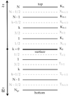 |
Fig. F.1 Discretisation of the atmosphere and ground into vertical levels. |
Appendix F.2 Discretisation of diffusion equations
The contribution of turbulent diffusion to the physical tendencies is computed every physical time step. Between the surface and the top of the atmosphere (internal levels corresponding to k = 1,…, N – 2), the discretised equations derived from Eq. (27) are given by
![${{X_{k + 1/2}^n - X_{k + 1/2}^{n - 1}} \over {{\rm{\Delta }}{t_{\rm{P}}}}} = {{\cal A} \over {m_{k + 1/2}^n}}\left[ {\rho _{k + 1}^nK_{X;k + 1}^n{{{\delta _z}X_{k + 1}^n} \over {\delta z_{k + 1}^n}} - \rho _k^nK_{X;k}^n{{{\delta _z}X_k^n} \over {\delta z_k^n}}} \right],$](/articles/aa/full_html/2022/07/aa43099-22/aa43099-22-eq245.png) (F.7)
(F.7)
with A the area of the surface parcels defined by horizontal intervals. We note that integer indices in subscripts indicate levels separating vertical intervals, and non-integer indices centres of vertical intervals (see Fig. F.1). For k = 0 (lower boundary condition),
![${{X_{1/2}^n - X_{1/2}^{n - 1}} \over {{\rm{\Delta }}{t_{\rm{P}}}}} = {{\cal A} \over {m_{1/2}^n}}\left[ {\rho _1^nK_{X;1}^n{{{\delta _z}X_1^n} \over {\delta z_1^n}} - {F_{{\rm{turb}}}}} \right],$](/articles/aa/full_html/2022/07/aa43099-22/aa43099-22-eq246.png) (F.8)
(F.8)
and, for k = N – 1 (upper boundary condition),
![${{X_{N - 1/2}^n - X_{N - 1/2}^{n - 1}} \over {{\rm{\Delta }}{t_{\rm{P}}}}} = - {{\cal A} \over {m_{N - 1/2}^n}}\left[ {\rho _{N - 1}^nK_{X;N - 1}^n{{{\delta _z}X_{N - 1}^n} \over {\delta z_{N - 1}^n}}} \right],$](/articles/aa/full_html/2022/07/aa43099-22/aa43099-22-eq247.png) (F.9)
(F.9)
where Fturb is the downward turbulent flux at the surface atmosphere interface Similarly as the equations of vertical diffusion, these equations are put into the form
 (F.10)
where we have introduced the coefficients
 (F.11)
This algebraic system is solved using the tri-diagonal matrix algorithm (Appendix H). We introduce, for k = 1,…, N – 1, the recursion relation
 (F.12)
where the coefficients ak and βk are given by
 (F.13)
with  . The αk and βk are first computed downwards starting from the upper boundary, where
 (F.14)
Then, the  are computed upwards, from k = 0 to k = N – 1, using the recursion relation given by Eq. (F.12) and starting from
 (F.15)
This allows the source terms of the momentum, thermodynamic, and moisture conservation equations to be calculated. Basically,
 (F.16)
Appendix G Soil heat transfer scheme
The 1D heat conduction equation given by Eq. (43) is solved by means of a finite difference method adapted from Appendix B.1 of Wang et al. (2016). The domain is discretised into Ngr vertical intervals of ũ following a geometric law of scale factor α (Fig. F.1). Denoting by k = 0,…, Ngr the vertical grid levels (k = 0 corresponding to the surface, and k = Ngr to the inner boundary of the domain), we express all of the ũk as functions of the thickness of the first layer ũ1. Literally, the depths of the full and intermediate levels are respectively given by
 (G.1)
(G.1)
 (G.2)
(G.2)
 |
Fig. G.1 Temporal integration scheme for the calculation of physical tendencies resulting from turbulent diffusion and soil heat conduction. The notation δt designates a physical timestep (δt = nP∆t with nP = 10). |
We take  and
and  . To solve the heat equation, we use an implicit scheme. The set of discretised equations is written, for
  as
as
![${{T_{k + 1{\rm{/}}2}^n - T_{k + 1{\rm{/}}2}^{n - 1}} \over {{\rm{\Delta }}{t_{\rm{P}}}}} = {1 \over {\delta {{\tilde u}_{k + 1{\rm{/}}2}}}}\left[ {{{{\delta _{\tilde u}}T_{k + 1}^n} \over {\delta {{\tilde u}_{k + 1}}}} - {{{\delta _{\tilde u}}T_k^n} \over {\delta {{\tilde u}_k}}}} \right],$](/articles/aa/full_html/2022/07/aa43099-22/aa43099-22-eq262.png) (G.3)
(G.3)
with  and the boundary conditions yield
![${{T_{1{\rm{/}}2}^n - T_{1{\rm{/}}2}^{n - 1}} \over {{\rm{\Delta }}{t_{\rm{P}}}}} = {1 \over {\delta {{\tilde u}_{1{\rm{/}}2}}}}\left[ {{{{\delta _{\bar u}}T_1^n} \over {\delta {{\tilde u}_1}}} + {1 \over {{I_{{\rm{gr}}}}}}\left( {\sum {F \downarrow \left( {{T_{\rm{s}}}} \right) - {\varepsilon _{\rm{s}}}{\sigma _{{\rm{SB}}}}T_{\rm{s}}^4} } \right)} \right],$](/articles/aa/full_html/2022/07/aa43099-22/aa43099-22-eq264.png) (G.4)
(G.4)
![${{T_{{N_{{\rm{g}}{{\rm{r}}^{ - 1{\rm{/}}2}}}}}^n - T_{{N_{{\rm{g}}{{\rm{r}}^{ - 1{\rm{/}}2}}}}}^{n - 1}} \over {{\rm{\Delta }}{t_{\rm{P}}}}} = - {1 \over {\delta {{\tilde u}_{{N_{{\rm{g}}{{\rm{r}}^{ - 1{\rm{/}}2}}}}}}}}\left[ {{{{\delta _{\tilde u}}T_{{N_{{\rm{g}}{{\rm{r}}^{ - 1}}}}}^n} \over {\delta {{\tilde u}_{{N_{{\rm{g}}{{\rm{r}}^{ - 1}}}}}}}}} \right].$](/articles/aa/full_html/2022/07/aa43099-22/aa43099-22-eq265.png)
Introducing the coefficients  and dk defined as
 (G.6)
(G.6)
the above equations (Eqs. (G.3-G.5)) are rewritten as
 (G.7)
(G.7)
and the system is put into the standard algebraic form
![$\left[ {\matrix{{{B_0}} \hfill & {{C_0}} \hfill & {} \hfill & {} \hfill & {} \hfill \cr {{A_1}} \hfill & {{B_1}} \hfill & {{C_1}} \hfill & {} \hfill & {} \hfill \cr {} \hfill & {{A_k}} \hfill & {{B_k}} \hfill & {{C_k}} \hfill & {} \hfill \cr {} \hfill & {} \hfill & {{A_{{N_{{\rm{g}}{{\rm{r}}^{ - 2}}}}}}} \hfill & {{B_{{N_{{\rm{g}}{{\rm{r}}^{ - 2}}}}}}} \hfill & {{C_{{N_{{\rm{g}}{{\rm{r}}^{ - 2}}}}}}} \hfill \cr {} \hfill & {} \hfill & {} \hfill & {{A_{{N_{{\rm{g}}{{\rm{r}}^{ - 1}}}}}}} \hfill & {{B_{{N_{{\rm{g}}{{\rm{r}}^{ - 1}}}}}}} \hfill \cr } } \right]\left[ {\matrix{{T_{1{\rm{/}}2}^n} \cr {T_{3{\rm{/}}2}^n} \cr {T_{k + 1{\rm{/}}2}^n} \cr {T_{{N_{{\rm{g}}{{\rm{r}}^{ - 3{\rm{/}}2}}}}}^n} \cr {T_{{N_{{\rm{g}}{{\rm{r}}^{ - 1{\rm{/}}2}}}}}^n} \cr } } \right] = \left[ {\matrix{{{b_0}} \cr {{b_1}} \cr {{b_k}} \cr {{b_{{N_{{\rm{g}}{{\rm{r}}^{ - 2}}}}}}} \cr {{b_{{N_{{\rm{g}}{{\rm{r}}^{ - 1}}}}}}} \cr } } \right],$](/articles/aa/full_html/2022/07/aa43099-22/aa43099-22-eq269.png) (G.8)
(G.8)
with the coefficients
 (G.9)
(G.9)
 (G.10)
The algebraic system given by Eq. (G.8) is solved by making use of Thomas algorithm (Appendix H). As a first step, the temperatures of two consecutive levels are linked together by the recursion relation
 (G.11)
where the coefficients αk and βk are defined, for  as
as
 (G.12)
with  At the inner boundary, the zero-flux condition leads to
 (G.13)
with  . Thus, the coefficients αk and βk are integrated upwards from the inner boundary.
As a second step, the equation of the surface boundary condition is put into the form
 (G.14)
where  and
and  are expressed as
![$C_{\rm{S}}^* = {I_{{\rm{gr}}}}{\rm{\Delta }}{t_{\rm{P}}}\left[ {{c_{1/2}} + {d_1}\left( {1 - {\alpha _1}} \right)} \right],$](/articles/aa/full_html/2022/07/aa43099-22/aa43099-22-eq281.png) (G.15)
(G.15)
![$F_{\rm{S}}^* = {I_{{\rm{gr}}}}{d_{\rm{1}}}\left[ {{\beta _1} + \left( {{\alpha _1} - 1} \right)T_{1/2}^{n - 1}} \right].$](/articles/aa/full_html/2022/07/aa43099-22/aa43099-22-eq282.png) (G.16)
(G.16)
In order to obtain an equation for the surface temperature, we proceed to a linear interpolation near the surface, which yields
 (G.17)
Combining the above equation with the recursion relation  -, we rearrange Eq. (G.14) into
 (G.18)
where the heat capacity per unit surface Cs and upcoming flux Fs are given by
 (G.19)
 (G.20)
In practice, this equation is linearised and solved with an implicit scheme. The parameters Cs and Fs can be set to constants if one does not wish to solve the vertical diffusion within the ground. This yields the surface temperature of the current step,  , which allows the temperatures at ground levels to be calculated using the recursion relation downwards.
Linearising and discretising the surface temperature evolution equation, given by Eq. (G.18), we obtain
 (G.21)
The downward heat flux associated with turbulent diffusion is expressed in its general form as
 (G.22)
which allows the surface temperature of the current step to be written as
 (G.23)
The evolution of the surface content of any tracer in liquid or solid phase can be described with a similar equation. It induces a source-sink term in the moisture conservation equation. In the case of temperature the downward turbulent flux is given by
 (G.24)
which is a function of the mean fields near the surface (see Eq. (33)). The coefficients A and B introduced in Eq. (G.22) are thus expressed as
 (G.25)
As shown by Fig. G.1, the soil heat transfer scheme is coupled with the turbulent diffusion scheme (Appendix F) through the equation of surface thermal evolution, which may lead to consistency issues. In order to preserve the consistency of the diffusion scheme from the lowest level of the atmosphere to the highest level of the ground conduction model, the two steps of the calculation are permuted in chronological order: temperatures are computed first, and the coefficients αk and βk are computed then, and conserved for the next step.
Simulations were run for various values of the ground thermal inertia given by Eq. (41)  for the Earth-like planet of Fig. 1 in order to investigate how numerical solutions depend on the soil thermal response. The two-day averaged temperature snapshots obtained from these simulations are shown by Fig. G.2. We observe that varying the ground thermal inertia over two orders of magnitude does not significantly alter the climate state of equilibrium. The change in Igr essentially affects the maximum wind speed, which varies by ~ 9%. The minimum surface temperature on the nightside, Tn, hardly varies, as it switches from 231.3 K for Igr = 102,103 J m−2 s−1/2 K−1 to 231.8 K for Igr = 104 J m−2 s−1/2 K−1. This insensitivity of mean fields to the soil vertical conduction is consistent with the fact that the circulation reaches a steady state where mean flows are essentially invariant in time. With variations, mean flows might be more substantially affected by vertical thermal diffusion in the soil.
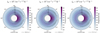 |
Fig. G.2 Two-day averaged temperature snapshots for various values of soil thermal inertia (see Eq. (41)). Left: Igr = 102 Jm−2 s−1/2 K−1. Middle: Igr = 103 J m−2 s−1/2 K−1. Right: Igr = 104 J m−2 s−1/2 K−1. Simulations were performed for the Earth-like case of Table 2 with a stellar irradiation of 1366 W irr2 and a 1 bar surface pressure, similar to as in Fig. 1. |
Appendix H Thomas algorithm for block tri-diagonal matrices
The tri-diagonal matrix algorithm (or the Thomas algorithm; Thomas 1949) can be used to solve a system of equations that involves a block tri-diagonal matrix of the form
![$\left[ {\matrix{ {{{\bf{B}}_0}} \hfill & {{{\bf{C}}_0}} \hfill & {} \hfill & {} \hfill & {} \hfill \cr {{{\bf{A}}_1}} \hfill & {{{\bf{B}}_1}} \hfill & {{{\bf{C}}_1}} \hfill & {} \hfill & {} \hfill \cr {} \hfill & {{{\bf{A}}_k}} \hfill & {{{\bf{B}}_k}} \hfill & {{{\bf{C}}_k}} \hfill & {} \hfill \cr {} \hfill & {} \hfill & {{{\bf{A}}_{N - 2}}} \hfill & {{{\bf{B}}_{N - 2}}} \hfill & {{{\bf{C}}_{N - 2}}} \hfill \cr {} \hfill & {} \hfill & {} \hfill & {{{\bf{A}}_{N - 1}}} \hfill & {{{\bf{B}}_{N - 1}}} \hfill \cr } } \right]\left[ {\matrix{ {{{\bf{x}}_0}} \cr {{{\bf{x}}_1}} \cr {{{\bf{x}}_k}} \cr {{{\bf{x}}_{N - 2}}} \cr {{{\bf{x}}_{N - 1}}} \cr } } \right] = \left[ {\matrix{ {{{\bf{d}}_0}} \cr {{{\bf{d}}_1}} \cr {{{\bf{d}}_k}} \cr {{{\bf{d}}_{N - 2}}} \cr {{{\bf{d}}_{N - 1}}} \cr } } \right],$](/articles/aa/full_html/2022/07/aa43099-22/aa43099-22-eq295.png) (H.1)
(H.1)
where the Ak, Bk, Ck are sub-matrices indexed by k = 0,…, Ν–1, and the xk and dk vectors of appropriate dimensions. As a first step, the matrix is triangularised, meaning that the system is transformed into a system where the matrix is block triangular. The new system is written as
![$\left[ {\matrix{ 1 & {{{\bf{\Gamma }}_0}} & {} & {} & {} \cr {} & 1 & {{{\bf{\Gamma }}_1}} & {} & {} \cr {} & {} & 1 & {{{\bf{\Gamma }}_k}} & {} \cr {} & {} & {} & 1 & {{{\bf{\Gamma }}_{N - 2}}} \cr {} & {} & {} & {} & 1 \cr } } \right]\left[ {\matrix{ {{{\bf{x}}_0}} \cr {{{\bf{x}}_1}} \cr {{{\bf{x}}_k}} \cr {{{\bf{x}}_{N - 2}}} \cr {{{\bf{x}}_{N - 1}}} \cr } } \right] = \left[ {\matrix{ {{{\bf{\beta }}_0}} \cr {{{\bf{\beta }}_1}} \cr {{{\bf{\beta }}_k}} \cr {{{\bf{\beta }}_{N - 2}}} \cr {{{\bf{\beta }}_{N - 1}}} \cr } } \right].$](/articles/aa/full_html/2022/07/aa43099-22/aa43099-22-eq296.png) (H.2)
(H.2)
The matrices Γk and vectors βk are computed forwards using the recursion relations
 (H.3)
(H.3)
 (H.4)
(H.4)


As a second step, the solution vectors xk are computed backwards (backward sweep) using the recursion relation
 (H.7)
(H.7)
 (H.8)
(H.8)
Appendix I Interhemispheric mass flow rate
At the terminator (θ = 90° in TLCs), the total mass flow rate (i.e. mass that passes through the terminator annulus per unit of time in one direction) is given by
 (I.1)
(I.1)
The day night advection timescale tadv corresponds to the mean timescale necessary for one particle to accomplish one full cycle of the day night overturning circulation. It measures the renewal rate of the air and the strength of the cell. The smaller tadv and the faster air is advected from the dayside to the nightside. Introducing the total mass of the atmosphere  , this timescale can be defined as
 (I.2)
(I.2)
In sigma coordinates, the circulation timescale is expressed as
 (I.3)
(I.3)
the integral being performed at the terminator (θ = 90°).
References
- Arakawa, A., & Lamb, V.R. 1977, Gen. Circ. Models Atmos., 17, 173 [CrossRef] [Google Scholar]
- Auclair-Desrotour, P., & Heng, K. 2020, A&A, 638, A77 [NASA ADS] [CrossRef] [EDP Sciences] [Google Scholar]
- Auclair-Desrotour, P., Leconte, J., Bolmont, E., & Mathis, S. 2019a, A&A, 629, A132 [NASA ADS] [CrossRef] [EDP Sciences] [Google Scholar]
- Auclair-Desrotour, P., Leconte, J., & Mergny, C. 2019b, A&A, 624, A17 [NASA ADS] [CrossRef] [EDP Sciences] [Google Scholar]
- Barclay, T., Pepper, J., & Quintana, E.V. 2018, ApJS, 239, 2 [NASA ADS] [CrossRef] [Google Scholar]
- Barnes, R., Raymond, S.N., Jackson, B., & Greenberg, R. 2008, Astrobiology, 8, 557 [NASA ADS] [CrossRef] [Google Scholar]
- Blackadar, A.K. 1962, J. Geophys. Res., 67, 3095 [CrossRef] [Google Scholar]
- Bruhat, G. 1968, Thermodyn. Rev. A. Kastler, 6, 360 [Google Scholar]
- Buckingham, E. 1914, Phys. Rev., 4, 345 [CrossRef] [Google Scholar]
- Carone, L., Keppens, R., & Decin, L. 2014, MNRAS, 445, 930 [NASA ADS] [CrossRef] [Google Scholar]
- Correia, A.C.M., Boué, G., Laskar, J., & Rodriguez, A. 2014, A&A, 571, A50 [NASA ADS] [CrossRef] [EDP Sciences] [Google Scholar]
- Courant, R., Friedrichs, K., & Lewy, H. 1928, Math. Ann., 100, 32 [Google Scholar]
- Deitrick, R., Mendonça, J.M., Schroffenegger, U., et al. 2020, ApJS, 248, 30 [NASA ADS] [CrossRef] [Google Scholar]
- Deming, D., Seager, S., Winn, J., et al. 2009, PASP, 121, 952 [NASA ADS] [CrossRef] [Google Scholar]
- Ding, F., & Pierrehumbert, R.T. 2020, ApJ, 901, L33 [NASA ADS] [CrossRef] [Google Scholar]
- Dobrovolskis, A.R. 2009, Icarus, 204, 1 [CrossRef] [Google Scholar]
- Edson, A., Lee, S., Bannon, P., Kasting, J.F., & Pollard, D. 2011, Icarus, 212, 1 [CrossRef] [Google Scholar]
- Etheridge, D.M., Steele, L.P., Langenfelds, R.L., et al. 1996, J. Geophys. Res., 101, 4115 [NASA ADS] [CrossRef] [Google Scholar]
- Fanale, F.P., Salvail, J.R., Banerdt, W.B., & Saunders, R.S. 1982, Icarus, 50, 381 [NASA ADS] [CrossRef] [Google Scholar]
- Frierson, D.M.W., Held, I.M., & Zurita-Gotor, P. 2006, J. Atmos. Sci., 63, 2548 [NASA ADS] [CrossRef] [Google Scholar]
- Garratt, J.R. 1994, The Atmospheric Boundary Layer (Cambridge University press) [Google Scholar]
- Gerkema, T., & Zimmerman, J. 2008, Lecture Notes, Royal NIOZ, Texel [Google Scholar]
- Gill, A.E. 1980, Q.J.R. Meteorol. Soc., 106, 447 [CrossRef] [Google Scholar]
- Gillon, M., Triaud, A.H.M.J., Demory, B.-O., et al. 2017, Nature, 542, 456 [NASA ADS] [CrossRef] [Google Scholar]
- Gold, T., & Soter, S. 1969, Icarus, 11, 356 [NASA ADS] [CrossRef] [Google Scholar]
- Goldreich, P. 1966, AJ, 71, 1 [NASA ADS] [CrossRef] [Google Scholar]
- Grimm, S.L., Demory, B.-O., Gillon, M., et al. 2018, A&A, 613, A68 [NASA ADS] [CrossRef] [EDP Sciences] [Google Scholar]
- Hammond, M., & Lewis, N.T. 2021, Proc. Natl. Acad. Sci., 118, 2022705118 [NASA ADS] [CrossRef] [Google Scholar]
- Hammond, M., & Pierrehumbert, R.T. 2017, ApJ, 849, 152 [CrossRef] [Google Scholar]
- Hansen, J., Russell, G., Rind, D., et al. 1983, Monthly Weather Rev., 111, 609 [NASA ADS] [CrossRef] [Google Scholar]
- Haqq-Misra, J., Wolf, E.T., Joshi, M., Zhang, X., & Kopparapu, R.K. 2018, ApJ, 852, 67 [NASA ADS] [CrossRef] [Google Scholar]
- Harris, C.R., Millman, K.J., van der Walt, S.J., et al. 2020, Nature, 585, 357 [NASA ADS] [CrossRef] [Google Scholar]
- Held, I.M. 2005, Bull. Am. Meteorol. Soc., 86, 1609 [CrossRef] [Google Scholar]
- Heng, K. 2017, Exoplanetary Atmospheres: Theoretical Concepts and Foundations (Princeton University press) [Google Scholar]
- Heng, K., & Kopparla, P. 2012, ApJ, 754, 60 [NASA ADS] [CrossRef] [Google Scholar]
- Holtslag, A.A.M., & Boville, B.A. 1993, J. Climate, 6, 1825 [NASA ADS] [CrossRef] [Google Scholar]
- Hourdin, F. 1994, Note interne du LMD, 1 [Google Scholar]
- Hourdin, F., Le van, P., Forget, F., & Talagrand, O. 1993, J. Atmos. Sci., 50, 3625 [NASA ADS] [CrossRef] [Google Scholar]
- Hourdin, F., Musat, I., Bony, S., et al. 2006, Climate Dynamics, 27, 787 [NASA ADS] [CrossRef] [Google Scholar]
- Hunter, J.D. 2007, Comput. Sci. Eng., 9, 90 [Google Scholar]
- Hut, P. 1980, A&A, 92, 167 [NASA ADS] [Google Scholar]
- Hut, P. 1981, A&A, 99, 126 [NASA ADS] [Google Scholar]
- Ingersoll, A.P., & Dobrovolskis, A.R. 1978, Nature, 275, 37 [CrossRef] [Google Scholar]
- Innes, H., & Pierrehumbert, R.T. 2022, ApJ, 927, 38 [NASA ADS] [CrossRef] [Google Scholar]
- Joshi, M.M., Haberle, R.M., & Reynolds, R.T. 1997, Icarus, 129, 450 [NASA ADS] [CrossRef] [Google Scholar]
- Joshi, M.M., Elvidge, A.D., Wordsworth, R., & Sergeev, D. 2020, ApJ, 892, L33 [NASA ADS] [CrossRef] [Google Scholar]
- Kasahara, A. 1974, Monthly Weather Rev., 102, 509 [NASA ADS] [CrossRef] [Google Scholar]
- Kasting, J.F., Whitmire, D.P., & Reynolds, R.T. 1993, Icarus, 101, 108 [NASA ADS] [CrossRef] [Google Scholar]
- Koll, D.D.B. 2022, ApJ, 924, 134 [NASA ADS] [CrossRef] [Google Scholar]
- Koll, D.D.B., & Abbot, D.S. 2015, ApJ, 802, 21 [NASA ADS] [CrossRef] [Google Scholar]
- Koll, D.D.B., & Abbot, D.S. 2016, ApJ, 825, 99 [NASA ADS] [CrossRef] [Google Scholar]
- Koll, D.D.B., & Komacek, T.D. 2018, ApJ, 853, 133 [NASA ADS] [CrossRef] [Google Scholar]
- Komacek, T.D., & Showman, A.P. 2016, ApJ, 821, 16 [CrossRef] [Google Scholar]
- Kopparapu, R.K., Ramirez, R., Kasting, J.F., et al. 2013, ApJ, 765, 131 [NASA ADS] [CrossRef] [Google Scholar]
- Kopparapu, R.K., Wolf, E.T., Arney, G., et al. 2017, ApJ, 845, 5 [NASA ADS] [CrossRef] [Google Scholar]
- Lacis, A.A. 1975, J. Atmos. Sci., 32, 1107 [NASA ADS] [CrossRef] [Google Scholar]
- Lacis, A.A., & Oinas, V. 1991, J. Geophys. Res., 96, 9027 [NASA ADS] [CrossRef] [Google Scholar]
- Lauritzen, P.H., Jablonowski, C., Taylor, M.A., & Nair, R.D. 2011, Numerical techniques for global atmospheric models, 80 (Springer Science & Business Media) [Google Scholar]
- Lebonnois, S., Hourdin, F., Eymet, V., et al. 2010, J. Geophys. Res. (Planets), 115, E06006 [CrossRef] [Google Scholar]
- Leconte, J., Forget, F., Charnay, B., et al. 2013, A&A, 554, A69 [NASA ADS] [CrossRef] [EDP Sciences] [Google Scholar]
- Leconte, J., Wu, H., Menou, K., & Murray, N. 2015, Science, 347, 632 [NASA ADS] [CrossRef] [Google Scholar]
- Lee, U., & Saio, H. 1997, ApJ, 491, 839 [Google Scholar]
- Levrard, B., Winisdoerffer, C., & Chabrier, G. 2009, ApJ, 692, L9 [NASA ADS] [CrossRef] [Google Scholar]
- Majewski, D., Liermann, D., Prohl, P., et al. 2002, Monthly Weather Rev., 130, 319 [CrossRef] [Google Scholar]
- Matsuno, T. 1966a, J. Meteorol. Soc. Jpn., 44, 76 [NASA ADS] [CrossRef] [Google Scholar]
- Matsuno, T. 1966b, J. Meteorol. Soc. Jpn., 44, 25 [NASA ADS] [CrossRef] [Google Scholar]
- McKay, C.P., Pollack, J.B., & Courtin, R. 1991, Science, 253, 1118 [NASA ADS] [CrossRef] [Google Scholar]
- Meija, J., Coplen, T.B., Berglund, M., et al. 2016, Pure Appl. Chem., 88, 265 [CrossRef] [Google Scholar]
- Mendonça, J.M., & Buchhave, L.A. 2020, MNRAS, 496, 3512 [CrossRef] [Google Scholar]
- Mendonça, J.M., Grimm, S.L., Grosheintz, L., & Heng, K. 2016, ApJ, 829, 115 [CrossRef] [Google Scholar]
- Mendonça, J.M., Tsai, S.-M., Malik, M., Grimm, S.L., & Heng, K. 2018, ApJ, 869, 107 [CrossRef] [Google Scholar]
- Menou, K., Cho, J.Y.K., Seager, S., & Hansen, B.M.S. 2003, ApJ, 587, L113 [NASA ADS] [CrossRef] [Google Scholar]
- Merlis, T.M., & Schneider, T. 2010, J. Adv. Model. Earth Syst., 2, 13 [Google Scholar]
- Mohr, P.J., Newell, D.B., & Taylor, B.N. 2016, Rev. Mod. Phys., 88, 035009 [NASA ADS] [CrossRef] [Google Scholar]
- Pauluis, O., Czaja, A., & Korty, R. 2008, Science, 321, 1075 [NASA ADS] [CrossRef] [Google Scholar]
- Payne, M.J., & Lodato, G. 2007, MNRAS, 381, 1597 [NASA ADS] [CrossRef] [Google Scholar]
- Peale, S.J. 1977, in IAU Colloq. 28: Planetary Satellites, 87 [Google Scholar]
- Pierrehumbert, R.T. 1995, J Atmos. Sci., 52, 1784 [NASA ADS] [CrossRef] [Google Scholar]
- Pierrehumbert, R.T. 2010, Principles of Planetary Climate (University of Chicago) [CrossRef] [Google Scholar]
- Pierrehumbert, R.T., & Ding, F. 2016, Proc. R. Soc. Lond. A, 472, 20160107 [NASA ADS] [Google Scholar]
- Pierrehumbert, R.T., & Hammond, M. 2019, Annu. Rev. Fluid Mech., 51, 275 [NASA ADS] [CrossRef] [Google Scholar]
- Polvani, L.M., & Kushner, P.J. 2002, Geophys. Res. Lett., 29, 1114 [NASA ADS] [CrossRef] [Google Scholar]
- Press, W.H., Teukolsky, S.A., Vetterling, W.T., & Flannery, B.P. 2007, Numerical Recipes, 3rd edn.: The Art of Scientific Computing (Cambridge University Press) [Google Scholar]
- Ragazzoni, R., Magrin, D., Rauer, H., et al. 2016, SPIE Conf. Ser., 9904, 990428 [NASA ADS] [Google Scholar]
- Raymond, S.N., Scalo, J., & Meadows, V.S. 2007, ApJ, 669, 606 [NASA ADS] [CrossRef] [Google Scholar]
- Rhines, P.B. 1975, J. Fluid Mech., 69, 417 [NASA ADS] [CrossRef] [Google Scholar]
- Robinson, T.D., & Catling, D.C. 2012, ApJ, 757, 104 [CrossRef] [Google Scholar]
- Sadourny, R. 1975a, J. Atmos. Sci., 32, 2103 [NASA ADS] [CrossRef] [Google Scholar]
- Sadourny, R. 1975b, J. Atmos. Sci., 32, 680 [NASA ADS] [CrossRef] [Google Scholar]
- Sergeev, D.E., Lambert, F.H., Mayne, N.J., et al. 2020, ApJ, 894, 84 [NASA ADS] [CrossRef] [Google Scholar]
- Showman, A.P., & Guillot, T. 2002, A&A, 385, 166 [NASA ADS] [CrossRef] [EDP Sciences] [Google Scholar]
- Showman, A.P., & Polvani, L.M. 2011, ApJ, 738, 71 [NASA ADS] [CrossRef] [Google Scholar]
- Showman, A.P., Wordsworth, R.D., Merlis, T.M., & Kaspi, Y. 2013, Atmospheric Circulation of Terrestrial Exoplanets, eds. S.J. Mackwell, A.A. Simon-Miller, J.W. Harder, & M.A. Bullock, 277 [Google Scholar]
- Sobel, A.H., Nilsson, J., & Polvani, L.M. 2001, J. Atmos. Sci., 58, 3650 [CrossRef] [Google Scholar]
- Song, Q., Yang, J., Luo, H., Li, C., & Fu, S. 2021, ArXiv e-prints, [arXiv:2108.04143] [Google Scholar]
- Sukoriansky, S., Galperin, B., & Staroselsky, I. 2005, Phys. Fluids, 17, 085107 [NASA ADS] [CrossRef] [Google Scholar]
- Thomas, L.H. 1949, Watson Sci. Comput. Lab. Rept. (New York: Columbia University) 1 [Google Scholar]
- Thrastarson, H.T., & Cho, J.Y.-K. 2011, ApJ, 729, 117 [NASA ADS] [CrossRef] [Google Scholar]
- Tomita, H., & Satoh, M. 2004, Fluid Dyn. Res., 34, 357 [NASA ADS] [CrossRef] [Google Scholar]
- Tsai, S.-M., Dobbs-Dixon, I., & Gu, P.-G. 2014, ApJ, 793, 141 [NASA ADS] [CrossRef] [Google Scholar]
- Turbet, M., Bolmont, E., Leconte, J., et al. 2018, A&A, 612, A86 [NASA ADS] [CrossRef] [EDP Sciences] [Google Scholar]
- Turbet, M., Fauchez, T.J., Sergeev, D.E., et al. 2021, Planet. Sci. J., submitted [arXiv:2109.11457] [Google Scholar]
- Vallis, G.K. 2006, Atmos. Oceanic Fluid Dyn., 770 [Google Scholar]
- Virtanen, P., Gommers, R., Oliphant, T.E., et al. 2020, Nat. Methods, 17, 261 [NASA ADS] [CrossRef] [Google Scholar]
- Wang, H., & Wordsworth, R. 2020, ApJ, 891, 7 [NASA ADS] [CrossRef] [Google Scholar]
- Wang, F., Cheruy, F., & Dufresne, J.L. 2016, Geoscientific Model Dev., 9, 363 [NASA ADS] [CrossRef] [Google Scholar]
- Wordsworth, R. 2015, ApJ, 806, 180 [NASA ADS] [CrossRef] [Google Scholar]
- Wordsworth, R., Forget, F., & Eymet, V. 2010a, Icarus, 210, 992 [CrossRef] [Google Scholar]
- Wordsworth, R.D., Forget, F., Selsis, F., et al. 2010b, A&A, 522, A22 [NASA ADS] [CrossRef] [EDP Sciences] [Google Scholar]
- Yang, J., & Abbot, D.S. 2014, ApJ, 784, 155 [NASA ADS] [CrossRef] [Google Scholar]
- Yao, M.-S., & Stone, P.H. 1987, J. Atmos. Sci., 44, 65 [NASA ADS] [CrossRef] [Google Scholar]
- Yaws, C.L. 1996, Handbook of Thermodynamic Diagrams: Organic compounds C to C4 (Gulf Publishing Company) [Google Scholar]
- Zhang, X., & Showman, A.P. 2017, ApJ, 836, 73 [NASA ADS] [CrossRef] [Google Scholar]
Sensible heating designates surface-atmosphere heat exchanges due to the vertical turbulent diffusion generated by friction of mean flows against the planet’s surface within the surface layer in dry thermodynamics. This mechanism is distinct from latent heat exchanges, which designates the energy exchanges resulting from the change of phase of a condensable substance (e.g. Pierrehumbert 2010, Sect. 6.3).
In Wordsworth (2015), the atmosphere is assumed to be transparentin the visible and the mean cosine of the propagation angle in the infrared is set to  . As a consequence, the effective absorption coefficient κL of Eq. (25) is exactly twice larger than Wordsworth’s value, the optical depths being equal.


The global Courant number given by Eq. (A.17) should be multiplied by the number of horizontal cells to obtain the Courant number used in the CFL (Courant, Friedrichs, and Lewy) numerical stability condition (Courant et al. 1928).
All Tables
Physics described by the four studied instances of the meta-model and the THOR 3D GCM.
All Figures
|
Fig. 1 Two-day averaged snapshots of pressure (left), temperature (middle), and vertical wind speed (right) distributions for the 1 bar-atmosphere of an Earth-sized tidally locked planet (Earth-like case of Table 2) with a stellar irradiation of 1366 W m−2 after convergence (t = 400 days). From bottom to top: OD (1 × 1 grid), 1D (1 × 50 grid), 1.5D (2 × 50 grid), and 2D (32 × 50 grid) instances of the meta-model. The sub-stellar point corresponds to θ = 0° and the anti-stellar point to θ = 180°. |
| In the text | |
|
Fig. 2 Two-day averaged potential temperature field in the Earth-like case of Table 2 with ps = 1 bar and F⋆ = 1366 W m−2. Plotted values belong to the interval [248 K, 376 K]. Outside of this interval, the colour is set to that of the closest bound. The 2D instance of the meta-model (32 × 50 grid) is used. The latitudes 90° and −90° correspond to the sub-and anti-stellar points, respectively. |
| In the text | |
|
Fig. 3 Stability diagrams of Earth-sized tidally locked planets with Earth-like (left panels) and pure CO2 (right panels) atmospheres, and the associated minimum surface temperature. Quantities are plotted as functions of the stellar flux normalised by the Earth’s stellar flux, F⋆/F⊕ (horizontal axis), and the surface pressure, ps, in logarithmic scale (vertical axis). From bottom to top: 0D (1 × 1 grid), 1D (1 × 50 grid), 1.5D (2 × 50 grid), and 2D (32 × 50 grid) instances of the meta-model. Large red dots indicate simulations where the atmosphere remained stable, while small blue dots indicate atmospheric collapse. The dashed orange (or dotted pink) line indicates the collapse pressure pC;low (or pC;up) corresponding to the lower (or upper) bound of the nightside surface temperature predicted by Wordsworth’s analytic model and given by Eq. (11). |
| In the text | |
|
Fig. 4 Stability diagrams of Earth-sized tidally locked planets hosting Earth-like (left panels) and pure CO2 (right panels) atmospheres, with turbulent diffusion (TD, four bottom panels) and without turbulent diffusion (NTD, four top panels), superimposed on the maps of various quantities. From bottom to top: day-night advection timescale with turbulent diffusion, day-night advection timescale with turbulent diffusion over the lower bound estimated analytically by Koll & Abbot (2016) using the heat engine theory, ratio of day-night advection timescales with and without turbulent diffusion, and nightside surface temperature difference between the cases with and without turbulent diffusion. The curves and symbols are the same as in Fig. 3. |
| In the text | |
|
Fig. 5 Maximum of Eulerian mean stream function (top) and its ratio over the scaling law (bottom) for Earth-sized planets hosting Earth-like (left panels) and pure CO2 (right panels) atmospheres. The two estimates of the Eulerian mean stream function are given by Eqs. (52) and (53), respectively. The curves and symbols are the same as in Fig. 3. |
| In the text | |
|
Fig. 6 Dayside and nightside surface temperatures vs. normalised equatorial Rossby deformation radius |
| In the text | |
|
Fig. A.1 Change of coordinate, ( |
| In the text | |
|
Fig. B.1 Staggered grid. In the adopted finite-volume method, the horizontal axis is divided into M intervals and the vertical axis into N intervals, which represents M × N cells (here, M = 5 and N = 4). Horizontal levels are indexed by j and vertical levels by k. The left and right boundaries of the physical domain correspond to |
| In the text | |
|
Fig. B.2 Subdivision of a surface area into two subsurface areas, A1 and A2 (light grey and grey regions). The big blue dots indicate the centres of horizontal intervals. The areas are calculated analytically by taking their dependence on colatitude into account. The configuration of the diagram corresponds to small horizontal intervals, where this dependence is approximately linear. |
| In the text | |
|
Fig. B.3 Time-differencing scheme implemented in the solver. The scheme is based on a leapfrog time step (e.g. Sect. 5.5.2 of Lauritzen et al. 2011), which is replaced by a Matsuno time step (Matsuno 1966a) every nMT = 5 steps. |
| In the text | |
|
Fig. C.1 Two-day averaged temperature snapshots for various values of the hyper-diffusion parameter (see Eq. (C.7)). Left: γ = 10−5. Middle: γ = 10−4. Right: γ = 10−3. Simulations were performed for the Earth-like case of Table 2 with a stellar irradiation of 1366 W m−2 and a 1 bar surface pressure, similar to as in Fig. 1. |
| In the text | |
|
Fig. D.1 Construction of the stable temperature profile in the convective adjustment scheme. An initially unstable region of the air column spreading from layer l1 to layer l2 is extended both downwards and upwards until the temperature profile is stable. At every step, the mass-averaged potential temperature of the region is adjusted to include the contribution of the current unstable layer. |
| In the text | |
|
Fig. E.1 Radiative transfer in double-grey approximation, as described in Appendix E. The equations for the shortwave and longwave radiative fluxes are solved separately. In each band, the coupled upward and downward fluxes are calculated by making use of the Thomas algorithm (see Appendix H). The superscript ′ designates the vertical gradient of the black body emission flux |
| In the text | |
|
Fig. F.1 Discretisation of the atmosphere and ground into vertical levels. |
| In the text | |
|
Fig. G.1 Temporal integration scheme for the calculation of physical tendencies resulting from turbulent diffusion and soil heat conduction. The notation δt designates a physical timestep (δt = nP∆t with nP = 10). |
| In the text | |
|
Fig. G.2 Two-day averaged temperature snapshots for various values of soil thermal inertia (see Eq. (41)). Left: Igr = 102 Jm−2 s−1/2 K−1. Middle: Igr = 103 J m−2 s−1/2 K−1. Right: Igr = 104 J m−2 s−1/2 K−1. Simulations were performed for the Earth-like case of Table 2 with a stellar irradiation of 1366 W irr2 and a 1 bar surface pressure, similar to as in Fig. 1. |
| In the text | |
Current usage metrics show cumulative count of Article Views (full-text article views including HTML views, PDF and ePub downloads, according to the available data) and Abstracts Views on Vision4Press platform.
Data correspond to usage on the plateform after 2015. The current usage metrics is available 48-96 hours after online publication and is updated daily on week days.
Initial download of the metrics may take a while.