| Issue |
A&A
Volume 663, July 2022
|
|
|---|---|---|
| Article Number | A80 | |
| Number of page(s) | 16 | |
| Section | Interstellar and circumstellar matter | |
| DOI | https://doi.org/10.1051/0004-6361/202243098 | |
| Published online | 18 July 2022 | |
And then they were two: Detection of non-thermal radio emission from the bow shocks of two runaway stars
1
Dublin Institute for Advanced Studies (DIAS),
31 Fitzwilliam Place,
Dublin 2,
Ireland
e-mail: This email address is being protected from spambots. You need JavaScript enabled to view it.
2
School of Physics, University College Dublin,
Belfield,
Dublin 4, Ireland
3
Instituto de Radioastronomía y Astrofísica (IRyA), Universidad Nacional Autónoma de México,
Morelia
58089,
Mexico
4
Max-Planck-Institut für Radioastronomie (MPIfR),
Auf dem Hügel 69,
53121
Bonn, Germany
5
Sternberg Astronomical Institute, Lomonosov Moscow State University,
Universitetskij Pr. 13,
Moscow
119992,
Russia
6
Space Research Institute, Russian Academy of Sciences,
Profsoyuznaya 84/32,
Moscow
117997, Russia
7
E. Kharadze Georgian National Astrophysical Observatory,
Abastumani
0301,
Georgia
Received:
12
January
2022
Accepted:
11
April
2022
Abstract
Context. In recent years, winds from massive stars have been considered promising sites for investigating relativistic particle acceleration. In particular, the resulting bow-shaped shocks from the interaction of the supersonic winds of runaway stars with interstellar matter have been intensively observed at many different wavelengths, from radio to γ-rays.
Aims. In this study we investigate the O4If star, BD+43° 3654, the bow shock of which is, so far, the only one proven to radiate both thermal and non-thermal emission at radio frequencies. In addition, we consider NGC 7635, the Bubble Nebula, as a bow shock candidate and examine its apex for indications of thermal and non-thermal radio emission.
Methods. We observed both bow shocks in radio frequencies with the Very Large Array (VLA) in the C and X bands (4–8 GHz and 8–12 GHz) and with the Effelsberg telescope at 4–8 GHz. We analysed single-dish and interferometric results individually, in addition to their combined emission, obtained spectral index maps for each source, and calculated their spectral energy distributions. Results. We find that both sources emit non-thermal emission in the radio regime, with the clearest evidence for NGC 7635, whose radio emission has a strongly negative spectral index along the northern rim of the bubble. We present the first high-resolution maps of radio emission from NGC 7635, finding that the morphology closely follows the optical nebular emission. Our results are less conclusive for the bow shock of BD+43° 3654, as its emission becomes weaker and faint at higher frequencies in VLA data. Effelsberg data show a much larger emitting region (albeit a region of thermal emission) than is detected with the VLA for this source.
Conclusions. Our results extend the previous radio results from the BD+43° 3654 bow shock to higher frequencies, and with our NGC 7635 results we double the number of bow shocks around O stars with detected non-thermal emission, from one to two. Modelling of the multi-wavelength data for both sources shows that accelerated electrons at the wind termination shock are a plausible source for the non-thermal radio emission, but energetics arguments suggest that any non-thermal X-ray and γ-ray emission could be significantly below existing upper limits. Enhanced synchrotron emission from compressed galactic cosmic rays in the radiative bow shock could also explain the radio emission from the BD+43° 3654 bow shock, but not from NGC 7635. The non-detection of point-like radio emission from BD+43° 3654 puts an upper limit on the mass-loss rate of the star that is lower than values quoted in the literature.
Key words: stars: massive / stars: winds / outflows / radio continuum: ISM / shock waves / radiation mechanisms: non-thermal / acceleration of particles
© M. Moutzouri et al. 2022
 Open Access article, published by EDP Sciences, under the terms of the Creative Commons Attribution License (https://creativecommons.org/licenses/by/4.0), which permits unrestricted use, distribution, and reproduction in any medium, provided the original work is properly cited.
This article is published in open access under the Subscribe-to-Open model. This email address is being protected from spambots. You need JavaScript enabled to view it. to support open access publication.
1 Introduction
OB-runaway stars are an unusual group of stars (about only 20% of O and B types; Fujii & Portegies Zwart 2011) that are ejected from their parent clusters and travel through the interstellar medium (ISM) with stellar velocities, υ⋆, of more than 30 km s−1 relative to the material they move through. Their strong winds, which have terminal velocities, varying from 1000 to 3000 km s−1, interact with the ISM hydrodynamically (Weaver et al. 1977). In particular, when υ⋆ > cs (cs is the sound speed of the ISM the star is passing through), the interaction of the stellar wind with the interstellar matter sweeps up and compresses the latter, creating an impressive, arc-shaped nebula, often referred to as a bow shock (Gull & Sofia 1979; van Buren & McCray 1988).
Bow shocks emit predominantly at mid-infrared wavelengths through thermal emission (TE) from dust that is radiatively heated by the wind-driving star (van Buren & McCray 1988; Meyer et al. 2014; Henney & Arthur 2019b). Infrared observations can, however, be difficult to interpret because they trace the dust and not the gas directly, and so the uncertainties in obtaining the gas density distribution are not small. The mid-infrared brightness is very sensitive to the assumed grain size distribution and composition (Pavlyuchenkov et al. 2013; Mackey et al. 2016; Katushkina & Izmodenov 2019). The emission scales with the dust density, and there are regions of parameter space where it is expected that dust and gas are not strongly coupled and the dust is a poor tracer of gas (Akimkin et al. 2015; Katushkina et al. 2018; Henney & Arthur 2019a).
Emission from nebular optical lines, such as Hα or [O iii], is fainter (Gull & Sofia 1979) but is a more reliable tracer of the gas conditions in the bow shock. Unfortunately, in this case, the stars driving bow shock nebulae tend to be very bright themselves, which may cause problems when trying to observe faint nebular emission. Furthermore, optical emission is significantly affected by interstellar extinction, which is often poorly constrained and sometimes patchy across an extended nebula (Deharveng et al. 2009).
Radio bremsstrahlung, on the other hand, is potentially a better observational tracer of the gas density because it is unaffected by extinction and because massive stars themselves are relatively faint radio sources. Radio can also be the best frequency range at which to detect diffuse non-thermal synchrotron radiation, which can be brighter than thermal bremsstrahlung at low frequencies (e.g. Benaglia et al. 2010). This possibility of detecting both TE and non-thermal emission (NTE) from bow shocks with radio observations can provide valuable constraints on the physical conditions of the thermal and relativistic particles in a bow shock (del Palacio et al. 2018), but one must first characterise the nature of the emission and separate TE from NTE1.
The NTE (synchrotron) arises from particles that are accelerated to relativistic energies in the termination shock of the stellar wind via diffusive shock acceleration (DSA; Drury 1983) and potentially also by synchrotron radiation from galactic cosmic rays (GCRs) compressed and deflected by the swept-up interstellar magnetic field in the bow shock (Cardillo et al. 2019). Following early theoretical calculations by Cesarsky & Montmerle (1983), there has recently been renewed interest in the possibility that winds from massive stars contribute significantly to the very high-energy GCR population (Aharonian et al. 2019). Of all the massive star systems without compact-object companions, only η Carinae (Tavani et al. 2009, H.E.S.S. Collaboration 2020) and γ2 Velorum (WR 11; Martí-Devesa et al. 2020; Pshirkov 2016), both colliding-wind binaries, have been detected in γ-rays.
So far, there has been no detection of NTE from bow shocks at very high energies (e.g. H.E.S.S. Collaboration 2018). Similarly, only upper limits exist in X-rays (Toalá et al. 2016, 2017). Nevertheless, at radio frequencies, there is the unique case of the bow shock associated with the star BD+43° 3654, from where previous studies (Benaglia et al. 2010, 2021, hereafter B10 and B21, respectively) detect both TE and NTE at low-gigahertz frequencies. Following the detection of synchrotron radiation from the Wolf-Rayet nebula G2.4+1.4 around WR 102 (Prajapati et al. 2019), and TE or NTE from the bow shock of the high-mass X-ray binary Vela X-1 (van den Eijnden et al. 2022), it becomes clear that radio observations are a promising avenue for identifying candidate bow shocks with strong NTE that can then be followed up at higher energies. What is more, the well-known Bubble Nebula around the star BD+60° 2522 was recently suggested to be a bow shock candidate by Green et al. (2019). Given that this source is very bright and has similar properties to the bow shock of BD+43° 3654, it was noted as another good candidate for detecting both TE and NTE, although X-ray observations again only resulted in upper limits (Toalá et al. 2020).
Motivated by these results, as well as the extended capabilities of the National Science Foundation’s (NSF) Karl G. Jansky Very Large Array (VLA; Perley et al. 2011), operated by the US National Radio Astronomy Observatory (NRAO), we investigate the bow shock of BD+43° 3654 and the nebula of BD+60° 2522 with radio observations at 4–12 GHz, applying several techniques to analyse their spectra. We extend the spectral coverage of previous BD+43° 3654 observations (B10, B21) to higher frequencies, where we expect TE to become more prominent. We also present the first high-resolution radio maps and spectral analysis of the nebula NGC 7635 around BD+60° 2522.
Given the difficulties in imaging extended diffuse sources with interferometers, it is important to obtain wide frequency coverage to more robustly characterise the thermal and non-thermal contributions to the observed emission. It is also important to assess how much flux is lost due to lack of sensitivity to large-scale uniform emission. For this reason we have supplemented our VLA observations with single-dish observations made with the Effelsberg 100-m radio telescope at 4–8 GHz.
In this paper, we present the results from our observations conducted with the VLA at the frequencies 4–12 GHz, single-dish data obtained with the Effelsberg telescope at similar frequencies, and a combination of both. In Sect. 2, we present our targets in detail, while in Sect. 3 we describe the observations. In Sect. 4, the results of the interferometric observations are presented; the single-dish observations and the combined results are shown in Sect. 4.4. We discuss our results in Sect. 5, and, finally, our conclusions are presented in Sect. 6.
Parameters of the massive stars driving the two bow shocks.
2 Targets
The bow shock around the massive star BD+43° 3654 and the nebula NGC 7635 around the star BD+60° 2522 are both windblown nebulae that produce bow shocks, and, as such, the properties of the central stars are important for determining the observational characteristics of the nebulae. Some relevant properties of both stars taken from literature are shown in Table 1.
2.1 BD+43° 3654
BD+43° 3654 is an O4If blue supergiant runaway star originating from the Cygnus OB2 association (Comerón & Pasquali 2007; Gvaramadze & Bomans 2008), located at a distance of 1.72 kpc (Gaia Collaboration 2021). With a stellar mass of ∼70 M⊙, a velocity of 69–100 km s−1 (see Sect. 2.3), and a wind speed of 2300 km s−1, BD+43° 3654 is a very massive runaway star. Its bow shock (hereafter referred to as BSBD43) is brightest in the infrared (e.g. Kobulnicky et al. 2016), but it is also visible at radio frequencies (B10, B21). B10 and B21 have found the bow shock to emit both TE and NTE, which, so far, is the sole evidence of non-thermal processes in radio for such shocks. Other studies have only obtained upper limits at higher energies (e.g. Toalá et al. 2016). From the brightness of the nebula and its size, the mean H number density of the ISM, nH, is estimated to be ∼15 cm−3 (del Palacio et al. 2018). The mass-loss rate, M, of this star is uncertain, with values ranging from 2.5 × 10⁻⁶ M⊙ yr−1 to 2 × 10⁻⁴ M⊙ yr−1 (Toalá et al. 2016); we assume 9 × 10⁻⁶ M⊙ yr−1 from del Palacio et al. (2018), appropriate for a star of its spectral type.
2.2 BD+60° 2522
BD+60° 2522 is an O6.5(n)fp star (Sota et al. 2011), surrounded by its wind-blown nebula, NGC 7635, commonly known as the Bubble Nebula (Christopoulou et al. 1995). The Bubble Nebula is prominent at infrared and optical wavelengths (Moore et al. 2002; Green et al. 2019). The high peculiar velocity of the star suggests that the nebula could be a bow shock (hereafter referred to as BSBD60). In fact, simulations by Green et al. (2019) have shown that the bow shock model is capable of reproducing the optical and infrared observations, further supporting the hypothesis. They have also suggested that similarities with BSBD43 make BSBD60 a good candidate for detecting both TE and NTE.
X-ray observations by Toalá et al. (2020) with the European Space Agency’s (ESA) X-ray Multi-Mirror Mission (XMM-Newton) detected BD+60° 2522 but no extended X-ray emission (neither TE nor NTE). The authors also estimate a mass of 27 M⊙ based on a distance of 2.5 kpc, but a newly measured parallax from Gaia Collaboration (2021) revised the distance to 3.0 kpc, and therefore the calculated mass should be rescaled to 39 M⊙. The only previous radio observations of NGC 7635 are low-resolution CO maps by Thronson et al. (1982); the observations we present here are the first high-resolution continuum maps at gigahertz frequencies.
BD+60° 2522 appears to be less massive, less evolved, and has a weaker wind than BD+43° 3654, and it is moving more slowly through the ISM. Nevertheless, it is moving through a denser ISM than BD+43° 3654 (estimated nH ∼50 cm−3, Green et al. 2019), and this gives the nebula a large emission measure resulting in bright optical line emission and continuum radio emission.
2.3 Space Velocity
We followed the method in Green et al. (2019) to calculate the space velocity of the two stars using Gaia Early Data Release 3 data (Gaia Collaboration 2021). We took the distance to the Galactic Centre of 8.0 kpc, the circular Galactic rotation velocity of 240 km s−1 (Reid et al. 2009), and for the solar peculiar velocity (U⊙, V⊙, W⊙) = (11.1, 12.2, 7.3) km s−1 (Schönrich et al. 2010). Using these, we obtain the peculiar velocity in the plane of the sky, υtr, and the peculiar radial velocity, υtr. For BD+43° 3654 we obtain υr = RV + 12.5 ± 0.1 km s−1 and for BD+60° 2522 υr = RV + 42 ± 2 km s−1, where RV is the heliocentric radial velocity with values taken from the references cited in the table. For both stars there are varying estimates of the radial velocity, with extreme differences between Kobulnicky et al. (2010) and Gaia Collaboration (2018) for the radial velocity of BD+43° 3654. This results in significant uncertainty in υr and the total peculiar velocity,  .
.
3 Radio Observations
3.1 Interferometric Data
In order to map the radio continuum of BSBD43 and BSBD60, observations were carried out with the VLA in New Mexico, on 16 and 19 November 2019 (Project ID, PID: 19B-105), covering the frequencies of 4–12 GHz. The mobile 27 antennas of the VLA are in a Y-shaped arrangement, while their distance can be modified to provide various combinations of angular resolution and surface brightness sensitivity in all the available frequencies. We chose the tightest configuration, D, with antennae separation from Bmin 35 m to Bmax 1 km, observed at the C and X band (4–8 GHz and 8–12 GHz, respectively) for optimal signal to noise ratio for such extended sources. The bands consisted of a number of 128 MHz wide spectral windows (SPWs; see Sect. 4.1.1). Both targets were observed once for each band for ∼30 min. For the flux density scale and bandpass calibration, 3C 48 was used, while for the phase and amplitude calibration, J2007+4029 and J2230+6946 were observed before and after each scan of BSBD43 and BSBD60 correspondingly. The raw data acquired from the observations were reduced using the VLA calibration pipeline included in the Common Astronomy Software Applications (CASA; McMullin et al. 2007). We used the CASA version 5.7 (6.1 for the pipeline) and the NRAO2 facilities in order to reduce our data.
3.2 Single-dish Data
There are two main difficulties when trying to measure extended emission accurately using an interferometer: the short-spacing problem (SSP) and the finite size of the primary beam (PB). For single-pointing observations like ours, the sensitivity of the measurement decreases with angular distance from the centre of the map because of the PB response. We can correct for this by scaling the map, but this also increases the noise level far from the map centre. What is more, beyond the first zero of the PB we cannot get any further useful information. The PB, since its size depends directly on the observed frequency, affects our observations at high frequencies for BSBD43, but less so for BSBD60 because it has a smaller angular extent. The SSP, on the other hand, arises because the antennas have a finite number of baselines and some short baselines are inaccessible because of the antenna layout. This can be potentially rectified by combining interferometric data with single dish observations (e.g. Rau et al. 2019) to help fill the uv-plane.
In September 2020, we observed the BSBD43 and BSBD60 with the S45 broadband receiver and the SPEctro-POLarimeter (SPECPOL) backend of the Effelsberg 100-m radio telescope3 at 4–8 GHz (PID: 86-20), reaching a sensitivity of ∼3 mJy beam−1. At the beginning of each observing session, pointing and focus were checked and corrected by performing cross scans of 3C 286. The same target was also adopted as our flux calibrator, with flux density of ∼7.3 Jy at 5 GHz (see Eq. (2) in Brunthaler et al. 2021). Each image was scanned in two orthogonal directions, and the ‘basket-weaving’ technique was used to reduce the scanning effects in the final image. For the lengths of the scans, they were designed to be 20’ for both BSBD43 and BSBD60. The overhead dumps beyond the designed 20’ scan are discarded in the image restoration, because they are not well sampled. The analysis was performed with the NOD3 software package (Müller et al. 2017) where the radio frequency interference (RFI) affecting certain frequency ranges is ‘flagged’ as part of the data editing process. The beam size is about 140″ at 5 GHz.
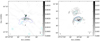 |
Fig. 1 (Non-PB-corrected) images of BSBD43 (left) and BSBD60 (right) in radio with contours at 4–12 GHz (VLA, black), at 1.4 GHz (NVSS, cyan, contour at 20 mJy), and infrared at 22 μm (WISE, blue). The star is symbolised with an asterisk and the VLA beam size at the bottom left with a solid black ellipse. The VLA contour levels are −5, 5, 10, 15, and 30 times the rms of 0.06 mJy beam−1 for BSBD43, whereas the rms for BSBD60 is 0.1 mJy beam−1. The contours for NVSS and WISE were chosen in order to highlight the most interesting features of each image. The grey scale shows the intensity in Jy beam−1. |
4 Radio Emission Analysis and Results
Following the imaging of BSBD43 and BSBD60, we estimated the spectral index of the bow shocks with several methods, both for our interferometric and single dish data, in order to determine the nature of their emission throughout the frequencies. In this section we present our analysis.
4.1 Imaging and Spectral Index Maps
4.1.1 Interferometric Data
Firstly, we imaged our targets for the whole frequency range of 4–12 GHz, by combining all 64 SPWs with a bandwidth of 128 MHz each (Fig. 1). The CASA task we used to do so, tclean, contains several image reconstruction algorithms, such as CLEAN (Högbom 1974), multi-scale (e.g. Cornwell 2008), as well as multi-scale multi-frequency deconvolution algorithms (MS-MFS; Rau & Cornwell 2011). Since BSBD43 and BSBD60 were both observed in multiple SPWs, the frequency dependence of the synthesised beam has to be accounted for, as well as the fact that the sources are very extended. With MS-MFS both were taken into account, leading us to choose it for our imaging process.
The final images (Fig. 1) were both cleaned for a diameter of 4 × FWHMPB, where FWHMPB is the full width half maximum (FWHM) of the PB of the instrument and it is estimated as
 (1)
(1)
where vc is the central frequency of the observations. For the full bandwidth of 4–12 GHz, vc = 8 GHz and FWHMPB = 5.25, which makes the field of view, FOV = 21′. In addition, we selected a cell size of 0″.7 and scales sizes of [0, 5, 10, 15, 20, 25, 50, 100, 200] pixels, with a small-scale bias of 0.9. The scale size 0 represents a point source, whereas the larger sizes represent wider features that are dominant in the image. The small-scale bias is “a numerical control to bias the solution towards smaller scales”4. Scales that were too large were ignored by the software.
The MS-MFS algorithm can also calculate the spectral index of the intensity map by modelling the spectrum of each flux component. After obtaining the spectral index maps, we manually corrected them for the PB response with the task widebandpbcor (which is not yet implemented in tclean for wide-band imaging). In order to do that, we fed the task with the raw data as well as the basename of our image files and selected the action calcalpha, which recalculates and corrects for PB response only the spectral index map and its error5. Next, we applied a mask of 5σ (which σ for BSBD43 is 0.06 mJy beam−1 and 0.2 mJy beam−1 for BSBD60) in order to bring forth the most significant areas of emission (Fig. 2, top). We repeated the steps for the spectral index error maps (Fig. 2, bottom).
As it can be seen from Fig. 2, both shocks seem to emit a mixture of TE and NTE. In particular, for BSBD43, a spectral index of ∼−1.5 appears to be consistent across the shock. Most of the areas of the shock that have very negative values (<−2) are also the areas where the error is > 1. Similarly, the spectral index of BSBD60 throughout the entire shock fluctuates around −1, while the errors are very small around the main area of emission.
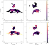 |
Fig. 2 Maps of the spectral index, α (top) and its uncertainty, αerr (bottom) for BSBD43 (left) and BSBD60 (right). Only pixels with significance above 5σ were selected, which is 0.3 mJy beam−1 for BSBD43 and 1 mJy beam−1 for BSBD60; white dotted contours surround errors equal to 0.5. The maps are scaled for α=[−2,0.5] and αerr = [0,1]. All maps are PB corrected. |
4.1.2 Single-dish Data
Effelsberg single-dish data have significantly lower resolution than VLA but are sensitive to emission at all spatial scales. The intensity maps from the Effelsberg observations of BSBD43 and BSBD60 are presented in Fig. 3, showing larger-scale features of the emitting regions than what is accessible with the VLA. The emission is partially resolved for BSBD43, revealing an extended arc of emission along the bow shock. For BSBD60, the Bubble is about the same size as the Effelsberg beam at 4.5 GHz, and so no details are visible. Here again the arc-shaped emission from the suspected bow shock is detected with Effelsberg, and traces the optical emission quite well (Green et al. 2019). In both observations, the H ii regions or bright-rimmed clouds outside of the bow shock are not resolved and contribute to the bow shock’s emission.
4.2 Morphology
BSBD43 (Fig. 1, left) appears to have a clear bow-like form, with main emission areas at the apex and western part of the shock. At the northern side of the shock there is a much brighter source. The data shows that it could be a photoionised region. Previous study (B21) reports the source as the H ii region 82.454+02.369 (Lockman 1989), although the spatial resolution of the Lockman observations does not allow us to distinguish between emission from this bright source and the bow shock.
The star itself is located south of the shock and we have not detected it, so it is represented instead with an asterisk in Fig. 1. Further south, two more radio point sources can be seen, NVSS J203418+435650 and WSRTGP 2031+4343 (Taylor et al. 1996). In the same figure, we have overplotted contours of the brightest emission from the NRAO VLA Sky Survey (NVSS) catalogue at 1.4 GHz (cyan, Condon et al. 1998) and Wide-field Infrared Survey Explorer (WISE) catalogue (blue, Wright et al. 2010) at 22μm. From this, we can see that a significant part of the eastern extension of the bow shock detected by WISE and NVSS is not detected by our VLA observations. This part is also visible in our single-dish observation (Fig. 3, left), but in that case every other detail is not present.
For BSBD60, the details seen in our high-resolution radio image (Fig. 1, right) correspond very well with the narrow-band nebular emission maps seen in optical with, for example, the Hubble Space Telescope (Moore et al. 2002)6. The bright arc on the north side of the Bubble corresponds to the brightest rim of the optical counterpart, and the bright-rimmed pillar seen projected onto the Bubble is the brightest emission region in radio. Further bright-rimmed clouds photoionised by BD+60° 2522 to the north-north-east of the Bubble are also detected with the VLA. Again, the star itself, BD+60° 2522, was not detected and is represented instead with an asterisk in Fig. 1. NVSS and WISE contours are also overplotted. We can see that their brightest emission matches with our observation. In contrast, the details of the bow shock are not visible in our Effelsberg observations (Fig. 3, right), where only the outer part of the Bubble is visible.
Both images were centred at the apex of each individual source; however, the BSBD60 emitting region does not extend as far from the phase centre as BSBD43 (∼160″ as opposed to the ∼300″ total width of BSBD43), contributing to better resolution of our observations. This is primarily due to the observing limits of the VLA. In particular, for our chosen D configuration, for C-band those limits are 12″-240″, while for X-band are 7″.2–145″. For sources with emission structures on scales larger than those limits the VLA cannot detect any emission, while for smaller structures the array acts like a single-dish instrument, smoothing the image to a lower resolution7. In our case, BSBD60 is within the observational limits of the array, but BSBD43 is not, resulting in loss of emission and resolution.
As a final remark on the morphology of the sources, we determined the standoff distance of the bow shocks, which can be calculated from (Baranov et al. 1970)
 (2)
(2)
where Mw is the mass-loss rate of the star, ρISM the density of surrounding ISM, ν⋆ the star velocity and cs speed of sound in the surrounding ISM. This characteristic scale of the bow shock gives the distance from the star where the ram pressure of the stellar wind equals the ram and thermal pressure of the ISM the star travels through. Given that nH is ≈ 15 cm−3 for BSBD43 and ≈ 50 cm−3 for BSBD60, and assuming standard ISM abundances, the ρISM can be calculated from (Green et al. 2019):
 (3)
(3)
where mp the proton mass. Combined with Eq. (2), RSO is 2′.72 for BSBD43 and 0′.42 for BSBD60. This can be compared to the angular distance of the bow shock from the star, as measured from the data image in CASA. This results in ∼4′, for BSBD43 and ∼0′.6, for BSBD60. In both cases, the calculated RSO is about 0.7 of the measured value. This is in agreement with Scherer et al. (2020), who find that RSO is consistent with the location of the wind termination shock, not the swept-up ISM.
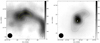 |
Fig. 3 Intensity map of the Effelsberg data at 4.5 GHz for BSBD43 (left) and BSBD60 (right). The beam size is represented as a solid black disc at the bottom left, while the star is represented with a white asterisk. The grey scale shows the intensity in mJy beam−1. The contours represent emission of 5, 10, and 15 σ, where σ is 30 mJy beam−1 and 10 mJy beam−1 for BSBD43 and BSBD60, respectively. The dotted yellow contours represent WISE emission at 22 μm, of 250 dn and 580 dn. |
4.3 Spectral Analysis
4.3.1 Interferometric Data
The spectral index appears to be fluctuating throughout the entire shock for both targets. In order to investigate this fluctuation more quantitatively, we split the data into smaller sub-bands of 1 GHz width and calculated their spectral energy distribution (SED) within each bow shock.
A single VLA sub-band has a width of 128 MHz. Therefore, by combining 8 sub-bands and following similar steps for imaging the full bandwidth, we can obtain an image of ∼1 GHz-width. First, we chose the shortest common uυ range (16kλ), then corrected for the PB and smoothed to the largest common beam, so we can compare them equally. Following, with the help of the CASA task, imstat, we integrated all of the flux within the 5σ contours, as shown in Fig. 1, for each bow shock (excluding other sources) as a function of frequency, and calculated the spectral index of the diffuse emission. The fluxes are presented in Table 2.
Both in the case of TE and NTE, the SED follows a power law:
 (4)
(4)
with α being the spectral index, its values ranging from −0.1 to +0.2 for TE, while for NTE it can reach negative values down to −0.8. We used the function curve_fit from the SciPy python library in order to fit the fluxes to the power law of Eq. (4) and calculate the average spectral index, assuming that all emission inside the limiting contour comes exclusively from the bow shock. The calculation yielded: αBSBD43 = −1.49 ± 0.08 and αBSBD60 = −0.76 ± 0.07 (Table 2), although we note that the obtained spectral index for BSBD43 is sensitive to the chosen dataset (see below for feathered data).
The fit to the VLA C- and X-band data is plotted at Fig. 4, where the errors of the flux are 5% calibration uncertainty (Perley & Butler 2017) and the frequency range is ±0.5 GHz. The upper and lower limit envelopes of the fit are determined from
![Mathematical equation: ${v^\alpha }{F_0} - \min \left[ {{\nu ^{\alpha - {\alpha _{{\rm{err}}}}}},{\nu ^{\alpha + {\alpha _{{\rm{err}}}}}}} \right]\left( {{F_0} + {F_{{\rm{err}}}}} \right),$](/articles/aa/full_html/2022/07/aa43098-22/aa43098-22-eq6.png) (5)
(5)
![Mathematical equation: ${\nu ^\alpha }{F_0} + \min \left[ {{\nu ^{\alpha + {\alpha _{{\rm{err}}}}}},{\nu ^{\alpha - {\alpha _{{\rm{err}}}}}}} \right]\left( {{F_0} - {F_{{\rm{err}}}}} \right),$](/articles/aa/full_html/2022/07/aa43098-22/aa43098-22-eq7.png) (6)
(6)
where α and αerr is the resulting spectral index from the fitting and its uncertainty, while F0 and Ferr are the flux normalisation and its uncertainty.
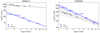 |
Fig. 4 Power-law fits to the flux within the 5σ contour of Fig. 1 from the VLA C- and X-band data (blue) and for the feathered VLA plus Effelsberg dataset (black) in Table 2. The horizontal error bars show the width of each sub-band, and the vertical error bars show the flux uncertainty The shaded regions show the 1σ bounds of the fit. |
4.3.2 Single Dish
The data were split into sub-bands of ∼200 MHz width to match the centre frequencies of the single VLA sub-bands. Their typical 1σ noise levels were about 6−6.5 mJy. From those frequency ranges, the ones where the final images in both cases (single-dish and interferometric data) had acceptable noise-to-signal ratios were chosen, namely 4.5, 4.7, 5, 5.4, 5.6, 6.6, and 7.6 GHz.
In order to derive the spectral index from the single-dish observations, we smooth all the images to the common angular resolution of 152". The temperature-temperature (TT) plot is widely used in single-dish observations to estimate the spectral index of extended sources (Turtle et al. 1962), and is thus adopted as our approach. The TT plot between the continuum emission at 4.487 GHz and 7.639 GHz is shown in the top panel of Fig. 5 where we only take the peak flux density of >50 mJy at 4.487 GHz into account and a 10% flux calibration has been included. Defining TΒ(ν) ∼ vβ where TB(v) is the brightness temperature at frequency ν and β is the brightness temperature spectral index, we obtain β = −2.20 ± 0.04 and β = −2.31 + 0.02 for BSBD43 and BSBD60 by the linear fit to the data points, respectively. We also apply this method to different pairs of the Effelsberg continuum images, which vary within in the range from −2.30 to −2.00 for BSBD43 and from −2.41 to −2.18 for BSBD60. The variation may arise from the calibration uncertainties.
In order to minimise the zero level uncertainties of the Effelsberg continuum images, we also make use of the background filtering method (Sofue & Reich 1979) to filter out the emission at the large scale of >10', which could arise from pervasive, diffuse, unrelated emission (i.e. originating in the Galactic disc). Then, we perform the linear fit to the data of each pixel to study the distribution of the spectral index. Assuming TB(v) = T5vβ where T5 is the brightness temperature at 5 GHz, we use the emcee code (Foreman-Mackey et al. 2013) to perform the Monte Carlo Markov chain calculations with the affme-invariant ensemble sampler (Goodman & Weare 2010) to fit all the Effelsberg continuum images. The uniform priors are assumed for T5 and β. The likelihood function is assumed to be  with
with
 (7)
(7)
where Ti,obs and Ti,mod are observed and modelled brightness temperatures, and σi is the standard deviation of Ti,obs The calculations are performed with 20 walkers and 8000 steps after the burn-in phase.
The spectral-index maps are shown in the top panel of Figs. 6 and 7, and an example of the Atting process is shown in the bottom panel of Figs. 6 and 7. The spectral index maps of both BSBD43 and BSBD60 suggest aβ of about −2.2, similar to the results derived from the TT plot. Taking the typical uncertainties of 0.2 in β (see the bottom panel of Fig. 6), we can infer that all of the emission is consistent with β ≈ −2.2, where α = β + 2(8), corresponding to TE. This is expected because Effelsberg is sensitive to large-scale diffuse emission from the photoionised Η ii region around the bow-shock-driving star, which is filtered out by the interferometric technique. Results for BSBD60 are very similar, consistent with TE.
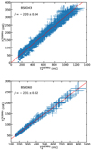 |
Fig. 5 Temperature-temperature plot of the bow shock of BSBD43 (top) and BSBD60 (bottom) using the Effelsberg continuum images at 4.487 GHz and 7.639 GHz. |
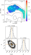 |
Fig. 6 Single-dish data analysis. Top: spectral index map of the bow shock of BD+43°3654, as seen with the Effelsberg telescope. As can be seen, the data are dominated by free-free emission. Bottom: posterior probability distributions of the fitted TB and β towards the position indicated by the cross in the middle panel. The maximum posterior possibility point in the parameter space is shown as an orange line. Contours denote the 0.5, 1.0, 1.5, and 2.0σ confidence intervals. |
4.4 Single-dish and Interferometry Data Combination
In order to combine our VLA data (hereafter IFD, for Inter-Ferometric Data) with our Effelsberg data (hereafter SDD, for single-dish data), we smoothed the images of each frequency to a common circular beam of FWHM 30″ for BSBD43, 20″ for BSBD60, and 155″ for all SDD. Next, we combined the IFD and SDD using the CASA task, feather (Rau et al. 2019), and converted the results into MJy sr−1. The data for the central frequency 7.6 GHz were omitted from the analysis of BSBD60 because the S/N was too low. All the results are shown in Figs. 8 and 9.
The feathering adds to the flux of BSBD43 (Fig. 8), especially to the SE of the apex of the shock, which agrees with the data from WISE and NVSS (Fig. 1, left). On the other hand, the feathering has not added any significant information for BSBD60 (Fig. 9).
Similarly, we calculated the SEDs for the feathered results as well as C-band only for the respective frequencies, and the results are summarised in Table 2. We find that α obtained from feathered maps is much closer to 0 (less negative) than IFD results for BSBD43, and the results are consistent with predominantly TE. Table 2 shows that the unphysically negative α = −1.49 + 0.08 that we obtained for the total VLA emission from the BSBD43 is changed to α = −0.31 + 0.16 with the inclusion of Effelsberg data in the feathered dataset. Within the uncertainties this is now consistent with mostly TE. The large difference between the VLA and feathered results indicates that BSBD43 is so diffuse that the VLA is not sensitive to much of the emission, particularly at the higher frequencies (see the respective fluxes in Table 2).
For BSBD60, the feathered results are very similar to the IFD.
5 Discussion
Wind bubbles are surrounded by Η ii regions (Mackey et al. 2015) that are bright thermal radio sources, whereas the outer edge of the wind bubble should be the brightest in ΝΤΕ (del Valle & Pohl 2018). We expect, therefore, the SDD to be sensitive to the more homogeneous and large-scale emission from the surrounding Ηii region, while the IFD to be more sensitive to the ΝΤΕ, which is less extended and has more small-scale structures. This is evident in the case of BSBD43, where the addition of the SDD has increased the spectral index, especially the additional areas that seem to appear after the feathering (Fig. 8). This could be due to the fact that SDD is dominated by TE (presumably from the Η ii region) with Sν ∝ ν-0.1, and that the total flux from Effelsberg is significantly larger than that obtained from the VLA. This makes the results somewhat difficult to interpret, because the spectral index obtained from the 5σ contours is consistent with TE in the feathered dataset, whereas from the VLA data alone one would conclude that most of the bow shock is emitting ΝΤΕ.
There are two possibilities that could explain our results. Either the emitting region is too extended for our VLA observations to obtain an accurate spectral index and so the emission is thermal at 4−12 GHz, or the VLA is picking out small features in the bow shock that are non-thermal emitters, and these are difficult to see once the bright, large-scale TE from Effelsberg is folded in. Given the detection of ΝΤΕ at lower frequencies (B21), we favour the latter interpretation.
Contrarily, for BSBD60 (Fig. 9) not much new information is added because, due to the fact that the diameter of the nebula is similar to the Effelsberg beam size, the emitting region is completely unresolved by the SDD. Our results for BSBD60 are relatively straightforward to interpret: we have detected synchrotron emission from the northern rim of the stellar wind bubble, and a combination of intense TE and ΝΤΕ from the bright-rimmed cloud projected onto the bubble.
5.1 Comparison Between Sources and With Literature
Both BSBD43 and BSBD60 have been studied before in the radio range (e.g. BIO, Thronson et al. 1982), but only the latter has not been previously proved to emit ΝΤΕ in the radio frequencies. In our analysis, however, it is the only source with self-consistency and this could be mainly due to its spatial extend. The fact that BSBD60 is smaller in diameter than BSBD43 contributes to a much higher S/N in the VLA images. This becomes even more evident from a flux comparison of the 5σ emission from both bow shocks throughout the bandwidth (Table 3), where BSBD60 is up to 10 times brighter than BSBD43.
On the other hand, our results for BSBD43 do not agree entirely with previous radio studies (B10, B21), which suggest that the bow shock emits NTE. In our case, the overall spectral index is too negative to be explained by NTE (−1.6). From Fig. 4, it can be argued that for frequencies <7 GHz, the spectrum is less steep. In fact, α4−7GHz = −0.83 ± 0.19, which agrees with the results of B21 for contours of >2.3 mJy beam−1. This could be due to loss of flux in higher frequencies from the SSP.
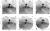 |
Fig. 8 Feathered results for BSBD43. All images appear within the limits of [0,1.2] MJy sr−1. The central frequency of each image is given at the top-right corner in GHz. |
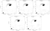 |
Fig. 9 Same as Fig. 8 but for BSBD60 only. All images appear within the limits of [0,10] MJy sr−1 for BSBD60. |
Flux as a function of photon energy per frequency for BSBD43 and BSBD60, including radio data from this work and the literature as well as X-ray and γ-ray upper limits from the literature.
5.2 Non-detection of the Stars
An additional comment can be made regarding the non-detection of the stars. Wright & Barlow (1975) state that for a star with a mass loss,  , at radio and infrared frequencies, v, the total observed flux can be calculated from the following:
 (8)
(8)
Here, for an ionised gas with ISM abundances, the ratio of electrons to ions is γ ≈ 1.2, the Gaunt factor is, with 20% accuracy, g ≈ 1.2 (Rybicki & Lightman 1986), the mean atomic gas weight is μ = 0.61 and Z = 1. The distance d is measured in kpc, wind speed υ∞, is in km s−1, and  is in M⊙ yr−1. For our observed frequencies, the mean value of the fluxes is calculated to be SBSBD43 ≈ 0.477 mJy and SBSBD60 ≈ 0.014 mJy. On the other hand, our observed 3σ upper limits are 0.18 mJy and 0.3 mJy, respectively. This implies two different outcomes foroursources. For BSBD60, our upper limit is much higher than the calculated value, meaning that the observational upper limit is consistent with the expected flux. For BSBD43, on the other hand, our upper limit implies that we should have detected this source (marginally) at the 2.7σ level, suggesting that
  might be overestimated. A reverse calculation of Eq. (8) using our 3σ upper limit results in a mass-loss rate of
  .
.
5.3 Modelling the Source of the Non-thermal Emission
There are at least two possible sources of NTE in bow shocks, electrons accelerated at the wind termination shock and radiating in the magnetic field of the shock (e.g. del Valle & Pohl 2018), and/or enhanced synchrotron emission from compression of the background GCR population and magnetic field in the radiative forward shock of the bow shock (Cardillo et al. 2019). Here we explore both possibilities.
5.3.1 Synchrotron and Inverse-Compton Emission Model
For both BSBD43 and BSBD60 we only have upper limits for NTE in X-ray and γ-ray bands, and with only radio detections one cannot predict a priori the level of the higher-energy radiation. Instead, we suppose that the actual X-ray and γ-ray flux is just below the upper limits quoted in Table 3, use the naima package (Zabalza 2015) to model the broadband SEDs, and compare the fitting results with the estimated physical conditions within the bow shocks. Considering the ambiguity of the shape of SED in the radio band, we build a box (grey colour, Fig. 10) in the radio band, covering all radio observations in this work. We assume a one-zone model with leptonic emission from electrons accelerated in the termination shock of the wind. The broadband SEDs and results of theoretical modelling are shown in Fig. 10. The X-ray and γ-ray data are upper limits taken from Table 3, except that for BSBD60 we consider the Fermi Large Area Telescope's point-source sensitivity as a nominal upper limit because there are no published results.
In the scope of this modelling, it is assumed that the electrons at the wind termination shock have the following energy distribution:
 (9)
(9)
where E is the energy of electrons, N(E) the number of electrons per unit energy, Γe is the power-law index, Ec and Emin describe the cut-off and the minimum energy of the electrons, and E0 is a normalisation constant. The total energy in relativistic electrons, We, is given by
 (10)
(10)
Considering the possible non-thermal origin of radio emission (B10, B21), it can be presumed that the lower energy band (i.e. from radio to X-ray) is due to synchrotron emission from the highly accelerated electrons in the magnetic field, B, along the bow shock. These electrons also interact with the ambient soft photon fields (from the star and the background) via inverse Compton (IC) scattering, producing high-energy emission from X-ray to γ-rays. The following radiation fields are considered: (i) cosmic microwave background (radiation temperature of 2.72 K, energy density of 1 eVcm−3); (ii) far-infrared dust emission (radiation temperature of 26.5 K, energy density of 0.415 eVcm−3); and (iii) stellar radiation, assuming a black-body with radiation temperature 40 700 Κ and energy density 2.4 × 1O−10 erg cm−3 for BSBD43, and radiation temperature 35 000 Κ and energy density 9.7 × 1O−10 erg cm−3 for BSBD60.
The energy density of the stellar field is obtained from the standoff distance of the bow shock and stellar luminosity of each object according to Urad = L/4πr2c. We use Rso ≈ 4′ (Sect. 4.2) and log L/L⊙ = 5.94 (Martins et al. 2005) for BD+43° 3654, and Rso ≈ 0′.6 (Sect. 4.2) and log L/L⊙ = 5.4 (Toalá et al. 2020) for BD+60° 2522.
The modelling best-fit parameters are presented Table 4. In both cases a hard power-law index (Γe ∼ 2) and a cutoff energy (Ec ∼ 1-3 TeV) are obtained. The hard spectrum is close to what is expected from DSA processes (e.g. Drury 1983). The total evaluated energy of electrons is We ∼ 1O47 erg in both cases. This can be compared with the total available energy processed through the wind termination shock. The wind power for each star  determines the total available energy:
 (11)
(11)
where tr is the time of residence for an accelerated particle in the shocked wind region, which can be calculated as tr ∼ Rso/ (del Palacio et al. 2018). Also, fvol is the fraction of the spherical region around the star that is responsible for the observable emission. For BD+43° 3654 the radio-bright emission cone has an opening angle θ ≈ 90° in the upstream direction, and for BD+60° 2522, θ ≈ 180°. If A is the surface area of the cone, then: A = 2πr2(l – cos θ/2) ⬄ fvol = A/(4πr2) = 0.5(1 - cos θ/2), evaluating to fvol ≈ 0.15 for BSBD43 and fvol ≈ 0.5 for BSBD60. Using the data from Table 1, we find Ew,bsbd43 = 1.5 × 1O47 erg and Ew,bsbd43 = 1.8 × 1O46 erg. Typically less than 1% of this energy goes to the accelerated electrons for standard shock-acceleration theories, and so we conclude that there is about 100 times (BSBD43) or 1000 times (BSBD60) less energy available than the We values obtained by the naima models. This implies that the actual level of non-thermal X-ray and γ-ray fluxes from these bow shocks is significantly below the upper limits from the literature, with the caveats that our modelling is a simple one-zone calculation with some quite uncertain parameters.
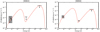 |
Fig. 10 Theoretical modelling of BSBD43 (left) and BSBD60 (right) by assuming a synchrotron and IC scenario and fitting using the naima package. Fit parameters are in Table 4. |
5.3.2 Compression of Galactic Electrons and Protons
Cardillo et al. (2019) attributed the gamma-ray access measured by Agile from Orion region to the compression of GCRs in the radiative bow shock of the massive OB star k-Ori moving through a region of a high ambient density. Here, we investigate if a similar compression of the Galactic electron and proton distribution can lead to detectable radio and gamma-ray emission.
The number density nad of adiabatically compressed cosmic rays is given by
 (12)
(12)
where r denotes the total shock-compression ratio and nISM the ambient cosmic ray density at momentum p (Tang 2019). We describe the spectrum of hadronic cosmic rays as a power law in total energy, modified at low energies by the particle speed, υp. The electron spectrum is a log-parabola at low energies,
 (13)
(13)
 (14)
(14)
Both electron and proton background spectra can be directly measured above a few GeV, where solar modulation is unimportant. The electron spectrum can be constrained by measurements of diffuse radio emission but the spectral slope of the proton spectrum at low energies remains unclear. At high energies the local cosmic ray spectrum has an index si = –2.75, which gives a spectrum harder than E−2 at low energies; we chose the normalisation in accordance with Moskalenko et al. (2002). For the electron spectrum, we fit the spectra given in Jaffe et al. (2011) for a galactocentric radius of 6.5 kpc with expression (14) as the spectrum shows a continuous change in the index below 4 GeV. The spectral index at high energies is found to be s2 = –3.04 and EB = 5 GeV. These spectra are compatible with direct observations of the electron spectra in the local ISM by Voyager 1, which also show spectra harder that s = 2.0 at low energies (Cummings et al. 2016).
It has to be noted that only low-energy particles can be efficiently compressed in the bow shock. Higher-energy particles have a larger mean-free path λ and cannot be confined when λ ≈ L, where L is the thickness of the compressed shell. Here, we assumed a thickness of L = 0.2 RSO. For the BSBD43, this means that particles with energies greater ≈ 15 GeV can only inefficiently be trapped.
The bow shock itself is likely radiative. Depending on the diffusion coefficient, even low-energetic cosmic rays might experience a compression ratio larger than the canonical value of 4, which is expected for a strong shock. Given the total compression due to radiative cooling of the downstream gas, values of Γe ≈ 1.25 might not be unreasonable. If the termination shock of the inner wind is the place of particle acceleration, local effects might significantly soften the electron spectra to values of Γe ⪢ 2 (Webb et al. 1985).
In addition to the parameters given in Table 1, we assumed a compression ratio at the forward shock of r = 20 and an ambient magnetic field strength of B0 = 5 µG. Since not all of the shock surface of the star can efficiently compress cosmic rays, we assumed a cone with a total opening angle of θ = 90° for the size of the compressing region. As a result, all emission was scaled by  ≈ 0.15 compared to a fully spherical emission geometry.
The model predicts the observed radio emission reasonably well for BSBD43 (see Fig. 11) and is at same time not violating the observational upper-limits on the gamma-ray emission. It has to be noted, nevertheless, that the hadronic gamma-ray emission represents the most optimistic scenario. Any lower ambient-medium density would reduce the hadronic gamma-ray emission while leaving the radio and IC emission unchanged, as long as the shock compression-ratio stays the same.
No reasonable set of parameters is able to reproduce the radio emission from BSBD60 in this scenario. This is mainly on account of the smaller separation between the star and the bow shock in this case. The small size of the emission region requires unreasonably strong magnetic fields (B0 ≥ 150 µG) and high compression factors (r ≥ 40).
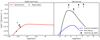 |
Fig. 11 Cosmic ray compression model for BSBD43, showing the predicted emission for radio (red), IC (blue), and pion-decay (black) emission based on the parameters in Table 1. The measured radio flux is denoted with stars and the gamma-ray upper limits by round markers. |
6 Conclusions
We report two new, high-resolution radio observations of bow shocks from runaway stars BD+43° 3654 (BSBD43) and BD+60° 2522 (BSBD60). We observed extended emission from both sources with the VLA and Effelsberg telescopes, at 4-12 GHz and 4-8 GHz, respectively. For BSBD43 we add higher frequency data to the results of B10 and B21, while for BSBD60 we present the first radio data since the 1970s. We then combined interferometric and single-dish data with the feather technique to further probe the nature of the emission of the bow shocks.
We have detected, for the first time, non-thermal radio emission from BSBD60, confirming the suggestion of Green et al. (2019) that this bow shock could be a bright non-thermal emitter. The emission traces a portion of the edge of the bubble very well, and the brightest region is the photoionised pillar projected behind the bubble. This pillar has the spectral index closest to TE, whereas the projected rim of the bubble has a more negative spectral index. In addition to its greater distance, BSBD60 appears quite compact compared to BSBD43, and so the inclusion of the Effelsberg data in the feathered dataset does not change the results significantly. Further interferometric radio observations at lower frequencies are needed to better characterise the emission and cleanly separate TE and NTE.
For BSBD43, our results are less conclusive: including only the VLA data, we find spectral indices that are so negative that they cannot be physical and must indicate some systematic loss of flux at high frequencies. Comparing the Effelsberg and VLA flux levels, we see that this is indeed the case, and the feathered dataset shows a mildly negative spectral index that could be consistent with TE or a combination of strong TE and weak NTE. The overall morphology of the VLA data is consistent with previous observations at lower frequency by B10 and B21. This suggests it is possible that the VLA observations are picking out small non-thermal emitting regions, which are concealed once the large-scale TE from Effelsberg is added, but this cannot be confirmed since we are missing flux at higher frequencies. Lower-spatial-resolution interferometric data are needed to test this hypothesis.
Finally, we modelled the source of the NTE in the two bow shocks with simple one-zone models of (i) high-energy electrons from shock acceleration at the wind termination shock and (ii) emission from GCRs compressed by the radiative forward shock of the bow shock. We find that the termination-shock model can explain the radio emission and is consistent with upper limits in X-rays and γ-rays. Using arguments based on the total energy available in non-thermal electrons, we show that the non-thermal X-ray and γ-ray emission could be well below current observational upper limits, for both sources. For the shock-compression model we find that it could explain the radio flux levels for BSBD43, and it predicts IC γ-ray emission about 0.5 dex below the Fermi upper limits. In the case of BSBD60, the bow shock is too small and the non-thermal radio emission cannot be explained by this model.
Acknowledgements
M.M. acknowledges funding from the Royal Society Research Fellows Enhancement Award 2017 (17/RS-EA/3468). J.M. acknowledges funding from a Royal Society-Science Foundation Ireland University Research Fellowship (14/RS-URF/3219, 20/RS-URF-R/3712). D.Z. and R.B. acknowledge funding from an Irish Research Council Starting Laureate Award (IRCLA\2017\83). This work is partly based on observations with the 100-m telescope of the MPIfR (Max-Planck-Institut für Radioastronomie) at Effelsberg. J.A.T. acknowledges funding from the UNAM DGAPA PAIIT (Mexico) project IA101622 and the Marcos Moshinsky Foundation (Mexico). The National Radio Astronomy Observatory is a facility of the National Science Foundation operated under cooperative agreement by Associated Universities, Inc. This publication makes use of data products from the Wide-field Infrared Survey Explorer, which is a joint project of the University of California, Los Angeles, and the Jet Propulsion Laboratory/California Institute of Technology, funded by the National Aeronautics and Space Administration. This work has made use of data from the European Space Agency (ESA) mission Gaia (https://www.cosmos.esa.int/gaia), processed by the Gaia Data Processing and Analysis Consortium (DPAC, https://www.cosmos.esa.int/web/gaia/dpac/consortium). Funding for the DPAC has been provided by national institutions, in particular the institutions participating in the Gaia Multilateral Agreement. The authors would like to thank the referee for their careful reading of our paper and constructive comments that improved the manuscript. Vasilii V. Gvaramadze very sadly passed away during the writing this paper; we will miss him.
Appendix A Analysis Including the H ii Regions Surrounding the Sources
It is worth discussing the difference it would make to our results if the H ii region above each of our sources was accounted for in our calculations for the spectral index. As it is mentioned in Sec. 4.3.1, we assumed for our calculations that only the bow shock is contributing to the total emission. It is, however, possible that the H ii region located at the northern part of our field of view can have an additional effect to the final results, especially given the large beam size of the Effelsberg data. Therefore, we included these sources (again for regions with flux above 5σ in the VLA map) and made an additional calculation of the spectral index for our data. The results are presented in Figs. B.1. For BSBD43, the spectral index becomes less negative, as expected because we add a presumably thermal source to the total. For BSBD60, the spectral index became more negative, likely because the VLA spectral index for these bright-rimmed clouds is strongly negative, albeit very uncertain (see Fig. 2). Here the results are inconclusive.
Appendix B Uv Range
The uυ range for each 1 GHz-wide band of BSBD43 is show in Figs. B.2. The equivalent plots for BSBD60 are omitted since they were similar, only different in amplitude. As it can be seen, all of them have a significant amount of information, thereby justifying the investigation of flux in the whole bandwidth.
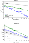 |
Fig. B.1 SED with H ii area above source included in VLA and feathered data. |
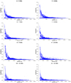 |
Fig. B.2 Intensity amplitude vs. uv wave (measured in the observed wavelength). Each plot represents a 1-gigahertz-wide band of our BSBD43 data. |
References
- Aharonian, F., Yang, R., & de Oña Wilhelmi, E. 2019, Nat. Astron., 3, 561 [Google Scholar]
- Akimkin, V. V., Kirsanova, M. S., Pavlyuchenkov, Y. N., & Wiebe, D. S. 2015, MNRAS, 449, 440 [NASA ADS] [CrossRef] [Google Scholar]
- Baranov, V. B., Krasnobaev, K. V., & Kulikovskii, A. G. 1970, Akad. Nauk SSSR Dokl., 194, 41 [NASA ADS] [Google Scholar]
- Benaglia, P., Romero, G. E., Martí, J., Peri, C. S., & Araudo, A. T. 2010, A&A, 517, L10 [NASA ADS] [CrossRef] [EDP Sciences] [Google Scholar]
- Benaglia, P., del Palacio, S., Hales, C., & Colazo, M. E. 2021, MNRAS, 503, 2514 [NASA ADS] [CrossRef] [Google Scholar]
- Brunthaler, A., Menten, K. M., Dzib, S. A., et al. 2021, A&A, 651, A85 [EDP Sciences] [Google Scholar]
- Cardillo, M., Marchili, N., Piano, G., et al. 2019, A&A, 622, A57 [NASA ADS] [CrossRef] [EDP Sciences] [Google Scholar]
- Cesarsky, C. J., & Montmerle, T. 1983, Space Sci. Rev., 36, 173 [NASA ADS] [CrossRef] [Google Scholar]
- Christopoulou, P. E., Goudis, C. D., Meaburn, J., Dyson, J. E., & Clayton, C. A. 1995, A&A, 295, 509 [NASA ADS] [Google Scholar]
- Comerón, F., & Pasquali, A. 2007, A&A, 467, L23 [NASA ADS] [CrossRef] [EDP Sciences] [Google Scholar]
- Condon, J. J., Cotton, W. D., Greisen, E. W., et al. 1998, AJ, 115, 1693 [Google Scholar]
- Cornwell, T. J. 2008, IEEE J. Sel. Top. Signal Process., 2, 793 [Google Scholar]
- Cummings, A. C., Stone, E. C., Heikkila, B. C., et al. 2016, ApJ, 831, 18 [CrossRef] [Google Scholar]
- Deharveng, L., Zavagno, A., Schuller, F., et al. 2009, A&A, 496, 177 [NASA ADS] [CrossRef] [EDP Sciences] [Google Scholar]
- del Palacio, S., Bosch-Ramon, V., Müller, A. L., & Romero, G. E. 2018, A&A, 617, A13 [NASA ADS] [CrossRef] [EDP Sciences] [Google Scholar]
- del Valle, M. V., & Pohl, M. 2018, ApJ, 864, 19 [NASA ADS] [CrossRef] [Google Scholar]
- Drury, L. O. 1983, Rep. Progr. Phys., 46, 973 [Google Scholar]
- Foreman-Mackey, D., Hogg, D. W., Lang, D., & Goodman, J. 2013, PASP, 125, 306 [Google Scholar]
- Fujii, M. S., & Portegies Zwart, S. 2011, Science, 334, 1380 [Google Scholar]
- Gaia Collaboration (Brown, A.G.A., et al.) 2018, A&A, 616, A1 [NASA ADS] [CrossRef] [EDP Sciences] [Google Scholar]
- Gaia Collaboration (Brown, A.G.A., et al.) 2021, A&A, 649, A1 [NASA ADS] [CrossRef] [EDP Sciences] [Google Scholar]
- Goodman, J., & Weare, J. 2010, Commun. Appl. Math. Comput. Sci., 5, 65 [Google Scholar]
- Green, S., Mackey, J., Haworth, T. J., Gvaramadze, V. V., & Duffy, P. 2019, A&A, 625, A4 [NASA ADS] [CrossRef] [EDP Sciences] [Google Scholar]
- Gull, T. R., & Sofia, S. 1979, ApJ, 230, 782 [CrossRef] [Google Scholar]
- Gvaramadze, V. V., & Bomans, D. J. 2008, A&A, 490, 1071 [NASA ADS] [CrossRef] [EDP Sciences] [Google Scholar]
- H.E.S.S. Collaboration (Abdalla, H., et al.) 2018, A&A, 612, A12 [NASA ADS] [CrossRef] [EDP Sciences] [Google Scholar]
- H.E.S.S. Collaboration (Abdalla, H., et al.) 2020, A&A, 635, A167 [NASA ADS] [CrossRef] [EDP Sciences] [Google Scholar]
- Henney, W. J., & Arthur, S. J. 2019a, MNRAS, 486, 4423 [Google Scholar]
- Henney, W. J., & Arthur, S. J. 2019b, MNRAS, 489, 2142 [NASA ADS] [CrossRef] [Google Scholar]
- Högbom, J. A. 1974, A&AS, 15, 417 [Google Scholar]
- Jaffe, T. R., Banday, A. J., Leahy, J. P., Leach, S., & Strong, A. W. 2011, MNRAS, 416, 1152 [NASA ADS] [CrossRef] [Google Scholar]
- Katushkina, O. A., & Izmodenov, V. V. 2019, MNRAS, 486, 4947 [Google Scholar]
- Katushkina, O. A., Alexashov, D. B., Gvaramadze, V. V., & Izmodenov, V. V. 2018, MNRAS, 473, 1576 [NASA ADS] [Google Scholar]
- Kobulnicky, H. A., Gilbert, I. J., & Kiminki, D. C. 2010, ApJ, 710, 549 [NASA ADS] [CrossRef] [Google Scholar]
- Kobulnicky, H. A., Chick, W. T., Schurhammer, D. P., et al. 2016, ApJS, 227, 18 [Google Scholar]
- Lockman, F. J. 1989, ApJS, 71, 469 [Google Scholar]
- Mackey, J., Gvaramadze, V. V., Mohamed, S., & Langer, N. 2015, A&A, 573, A10 [NASA ADS] [CrossRef] [EDP Sciences] [Google Scholar]
- Mackey, J., Haworth, T. J., Gvaramadze, V. V., et al. 2016, A&A, 586, A114 [NASA ADS] [CrossRef] [EDP Sciences] [Google Scholar]
- Maíz Apellániz, J., Sota, A., Arias, J. I., et al. 2016, ApJS, 224, 4 [CrossRef] [Google Scholar]
- Martí-Devesa, G., Reimer, O., Li, J., & Torres, D. F. 2020, A&A, 635, A141 [Google Scholar]
- Martins, F., Schaerer, D., & Hillier, D. J. 2005, A&A, 436, 1049 [NASA ADS] [CrossRef] [EDP Sciences] [Google Scholar]
- McMullin, J. P., Waters, B., Schiebel, D., Young, W., & Golap, K. 2007, in Astronomical Society of the Pacific Conference Series, Astronomical Data Analysis Software and Systems XVI, eds. R. A. Shaw, F. Hill, & D. J. Bell, 376, 127 [Google Scholar]
- Meyer, D. M. A., Mackey, J., Langer, N., et al. 2014, MNRAS, 444, 2754 [NASA ADS] [CrossRef] [Google Scholar]
- Moore, B. D., Walter, D. K., Hester, J. J., et al. 2002, AJ, 124, 3313 [NASA ADS] [CrossRef] [Google Scholar]
- Moskalenko, I. V., Strong, A. W., Ormes, J. F., & Potgieter, M. S. 2002, ApJ, 565, 280 [NASA ADS] [CrossRef] [Google Scholar]
- Müller, P., Krause, M., Beck, R., & Schmidt, P. 2017, A&A, 606, A41 [NASA ADS] [CrossRef] [EDP Sciences] [Google Scholar]
- Pavlyuchenkov, Y. N., Kirsanova, M. S., & Wiebe, D. S. 2013, Astron. Rep., 57, 573 [NASA ADS] [CrossRef] [Google Scholar]
- Perley, R. A., & Butler, B. J. 2017, ApJS, 230, 7 [NASA ADS] [CrossRef] [Google Scholar]
- Perley, R. A., Chandler, C. J., Butler, B. J., & Wrobel, J. M. 2011, ApJ, 739, L1 [Google Scholar]
- Prajapati, P., Tej, A., del Palacio, S., et al. 2019, ApJ, 884, L49 [NASA ADS] [CrossRef] [Google Scholar]
- Pshirkov, M. S. 2016, MNRAS, 457, L99 [NASA ADS] [CrossRef] [Google Scholar]
- Rau, U., & Cornwell, T. J. 2011, A&A, 532, A71 [NASA ADS] [CrossRef] [EDP Sciences] [Google Scholar]
- Rau, U., Naik, N., & Braun, T. 2019, AJ, 158, 3 [NASA ADS] [CrossRef] [Google Scholar]
- Reid, M. J., Menten, K. M., Zheng, X. W., Brunthaler, A., & Xu, Y. 2009, ApJ, 705, 1548 [NASA ADS] [CrossRef] [Google Scholar]
- Rybicki, G. B., & Lightman, A. P. 1986, Radiative Processes in Astrophysics (New York: John Wiley & Sons) [Google Scholar]
- Scherer, K., Baalmann, L. R., Fichtner, H., et al. 2020, MNRAS, 493, 4172 [Google Scholar]
- Schönrich, R., Binney, J., & Dehnen, W. 2010, MNRAS, 403, 1829 [NASA ADS] [CrossRef] [Google Scholar]
- Schulz, A., Ackermann, M., Buehler, R., Mayer, M., & Klepser, S. 2014, A&A, 565, A95 [NASA ADS] [CrossRef] [EDP Sciences] [Google Scholar]
- Sofue, Y., & Reich, W. 1979, A&AS, 38, 251 [NASA ADS] [Google Scholar]
- Sota, A., Maíz Apellániz, J., Walborn, N. R., et al. 2011, ApJS, 193, 24 [Google Scholar]
- Tang, X. 2019, MNRAS, 482, 3843 [NASA ADS] [CrossRef] [Google Scholar]
- Tavani, M., Sabatini, S., Pian, E., et al. 2009, ApJ, 698, L142 [NASA ADS] [CrossRef] [Google Scholar]
- Taylor, A. R., Goss, W. M., Coleman, P. H., van Leeuwen, J., & Wallace, B. J. 1996, ApJS, 107, 239 [NASA ADS] [CrossRef] [Google Scholar]
- Thronson, H. A.J., Lada, C.J., Harvey, P.M., & Werner, M.W. 1982, MNRAS, 201, 429 [CrossRef] [Google Scholar]
- Toalá, J. A., Oskinova, L. M., González-Galán, A., et al. 2016, ApJ, 821, 79 [CrossRef] [Google Scholar]
- Toalá, J. A., Oskinova, L. M., & Ignace, R. 2017, ApJ, 838, L19 [CrossRef] [Google Scholar]
- Toalá, J. A., Guerrero, M. A., Todt, H., et al. 2020, MNRAS, 495, 3041 [CrossRef] [Google Scholar]
- Turtle, A. J., Pugh, J. F., Kenderdine, S., & Pauliny-Toth, I. I. K. 1962, MNRAS, 124, 297 [NASA ADS] [CrossRef] [Google Scholar]
- van Buren, D., & McCray, R. 1988, ApJ, 329, L93 [NASA ADS] [CrossRef] [Google Scholar]
- van den Eijnden, J., Heywood, I., Fender, R., et al. 2022, MNRAS, 510, 515 [Google Scholar]
- Weaver, R., McCray, R., Castor, J., Shapiro, P., & Moore, R. 1977, ApJ, 218, 377 [Google Scholar]
- Webb, G. M., Axford, W. I., & Forman, M. A. 1985, ApJ, 298, 684 [CrossRef] [Google Scholar]
- Wright, A. E., & Barlow, M. J. 1975, MNRAS, 170, 41 [Google Scholar]
- Wright, E. L., Eisenhardt, P. R. M., Mainzer, A. K., et al. 2010, AJ, 140, 1868 [Google Scholar]
- Zabalza, V. 2015, in International Cosmic Ray Conference, 34th International Cosmic Ray Conference (ICRC2015), 34, 922 [Google Scholar]
In the following, TE and NTE refer to thermal and non-thermal radio emission, respectively, unless noted otherwise.
The NRAO is a facility of the NSF operated under cooperative agreement by Associated Universities, Inc.
The 100-metre telescope at Effelsberg is operated by the Max-PlanckInstitut für Radioastronomie (MPIFR) on behalf of the Max-Planck Gesellschaft (MPG).
The Rayleigh–Jeans law suggests Fv ∝ ν2T ∝ να and the temperature–frequency dependence defines T ∝ vβ, which gives α = β + 2.
All Tables
Flux as a function of photon energy per frequency for BSBD43 and BSBD60, including radio data from this work and the literature as well as X-ray and γ-ray upper limits from the literature.
All Figures
|
Fig. 1 (Non-PB-corrected) images of BSBD43 (left) and BSBD60 (right) in radio with contours at 4–12 GHz (VLA, black), at 1.4 GHz (NVSS, cyan, contour at 20 mJy), and infrared at 22 μm (WISE, blue). The star is symbolised with an asterisk and the VLA beam size at the bottom left with a solid black ellipse. The VLA contour levels are −5, 5, 10, 15, and 30 times the rms of 0.06 mJy beam−1 for BSBD43, whereas the rms for BSBD60 is 0.1 mJy beam−1. The contours for NVSS and WISE were chosen in order to highlight the most interesting features of each image. The grey scale shows the intensity in Jy beam−1. |
| In the text | |
|
Fig. 2 Maps of the spectral index, α (top) and its uncertainty, αerr (bottom) for BSBD43 (left) and BSBD60 (right). Only pixels with significance above 5σ were selected, which is 0.3 mJy beam−1 for BSBD43 and 1 mJy beam−1 for BSBD60; white dotted contours surround errors equal to 0.5. The maps are scaled for α=[−2,0.5] and αerr = [0,1]. All maps are PB corrected. |
| In the text | |
|
Fig. 3 Intensity map of the Effelsberg data at 4.5 GHz for BSBD43 (left) and BSBD60 (right). The beam size is represented as a solid black disc at the bottom left, while the star is represented with a white asterisk. The grey scale shows the intensity in mJy beam−1. The contours represent emission of 5, 10, and 15 σ, where σ is 30 mJy beam−1 and 10 mJy beam−1 for BSBD43 and BSBD60, respectively. The dotted yellow contours represent WISE emission at 22 μm, of 250 dn and 580 dn. |
| In the text | |
|
Fig. 4 Power-law fits to the flux within the 5σ contour of Fig. 1 from the VLA C- and X-band data (blue) and for the feathered VLA plus Effelsberg dataset (black) in Table 2. The horizontal error bars show the width of each sub-band, and the vertical error bars show the flux uncertainty The shaded regions show the 1σ bounds of the fit. |
| In the text | |
|
Fig. 5 Temperature-temperature plot of the bow shock of BSBD43 (top) and BSBD60 (bottom) using the Effelsberg continuum images at 4.487 GHz and 7.639 GHz. |
| In the text | |
|
Fig. 6 Single-dish data analysis. Top: spectral index map of the bow shock of BD+43°3654, as seen with the Effelsberg telescope. As can be seen, the data are dominated by free-free emission. Bottom: posterior probability distributions of the fitted TB and β towards the position indicated by the cross in the middle panel. The maximum posterior possibility point in the parameter space is shown as an orange line. Contours denote the 0.5, 1.0, 1.5, and 2.0σ confidence intervals. |
| In the text | |
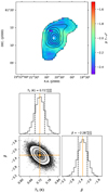 |
Fig. 7 Same as Fig. 6 but for BSBD60. |
| In the text | |
|
Fig. 8 Feathered results for BSBD43. All images appear within the limits of [0,1.2] MJy sr−1. The central frequency of each image is given at the top-right corner in GHz. |
| In the text | |
|
Fig. 9 Same as Fig. 8 but for BSBD60 only. All images appear within the limits of [0,10] MJy sr−1 for BSBD60. |
| In the text | |
|
Fig. 10 Theoretical modelling of BSBD43 (left) and BSBD60 (right) by assuming a synchrotron and IC scenario and fitting using the naima package. Fit parameters are in Table 4. |
| In the text | |
|
Fig. 11 Cosmic ray compression model for BSBD43, showing the predicted emission for radio (red), IC (blue), and pion-decay (black) emission based on the parameters in Table 1. The measured radio flux is denoted with stars and the gamma-ray upper limits by round markers. |
| In the text | |
|
Fig. B.1 SED with H ii area above source included in VLA and feathered data. |
| In the text | |
|
Fig. B.2 Intensity amplitude vs. uv wave (measured in the observed wavelength). Each plot represents a 1-gigahertz-wide band of our BSBD43 data. |
| In the text | |
Current usage metrics show cumulative count of Article Views (full-text article views including HTML views, PDF and ePub downloads, according to the available data) and Abstracts Views on Vision4Press platform.
Data correspond to usage on the plateform after 2015. The current usage metrics is available 48-96 hours after online publication and is updated daily on week days.
Initial download of the metrics may take a while.