| Issue |
A&A
Volume 663, July 2022
|
|
|---|---|---|
| Article Number | A89 | |
| Number of page(s) | 14 | |
| Section | The Sun and the Heliosphere | |
| DOI | https://doi.org/10.1051/0004-6361/202142761 | |
| Published online | 14 July 2022 | |
A new method to determine solar energetic particle anisotropies and their associated uncertainties demonstrated for STEREO/SEPT
1
Institut für Experimentelle und Angewandte Physik, Christian Albrechts-Universität zu Kiel, Kiel, Germany
e-mail: bruedern@physik.uni-kiel.de
2
Centre of Space Research, North-West University, North-West, South Africa
3
Department of Physics and Astronomy, University of Turku, Turku, Finland
Received:
26
November
2021
Accepted:
22
March
2022
Context. The shape of the pitch-angle distribution (PAD) of solar energetic particles (SEPs) can be used to infer information about their source and interplanetary transport. In modeling and observational studies of SEP events, these PADs are frequently applied to determine the anisotropy which is a proxy for the strength of the pitch-angle scattering during transport. For the determination of the PAD, derivation of the pitch angle of SEPs takes on a crucial role. For most instrument-sampled PADs, the particle’s pitch angle cannot be resolved directly but is usually approximated by considering the time-averaged in situ magnetic field direction, and the center viewing direction of the telescope. However, variations of the magnetic field, and the extent of the physical opening of the instrument lead to uncertainty on the determination of the pitch angle and therefore to uncertainty on the anisotropy and its interpretation.
Aims. In this work, we present a new method to determine a distribution of anisotropy values which allows us to estimate the corresponding uncertainty ranges. We apply our method to electron measurements by the Solar Electron and Proton Telescope on board each STEREO spacecraft.
Methods. We determined a distribution of anisotropy values by solving an inversion problem that takes into account the directional response of the instrument, the variation of the in situ magnetic field, and the stochastic nature of particle detection. Using 95% confidence intervals, we estimate the uncertainty on the anisotropy.
Results. The application of our method to a solar electron event observed by STEREO B on 14 August 2010 yields a maximum anisotropy of 1.9 with an uncertainty on the order of ±0.1. During the background period, the anisotropy shows strong fluctuations, and absolute uncertainties on the order of ±0.5 that are attributable to low counting statistics.
Key words: Sun: heliosphere / instrumentation: detectors / techniques: miscellaneous / Sun: particle emission
© ESO 2022
1. Introduction
The anisotropy of solar energetic particle (SEP) observations is an often-used quantity to obtain information about particle acceleration at the Sun, the injection of SEPs into space, and their transport through the interplanetary magnetic field. For instance, a long-lasting anisotropy indicates that particles are continuously injected into space, which can be an indicator of ongoing particle acceleration, for example by a coronal-mass-ejection-driven shock.
The anisotropy is a frequently applied quantity in observational (e.g., Dresing et al. 2014; Lario et al. 2014; Gómez-Herrero et al. 2015) and modeling studies (e.g., Dröge et al. 2014, 2016; Strauss et al. 2017a) of SEP events. From a physical point of view, the anisotropy expresses a snapshot of the preferred direction of a particle ensemble propagating with respect to the local direction of the interplanetary magnetic field. As SEPs are transported through the interplanetary magnetic field, their preferred direction, that is, their pitch angle, is subject to change. The instantaneous pitch angle of a particle propagating in a magnetic field is defined as the angle between its velocity vector and the local magnetic field vector. The nature of these pitch-angle changes can be stochastic, that is, scattering with fluctuations of the interplanetary magnetic field, or systematic, that is, because of the focusing effect of the radially decreasing interplanetary magnetic field. Mathematically, the first-order anisotropy A1 is defined as the first moment of the instantaneous pitch-angle-dependent particle distribution I(μ), where μ = cos(θ):
Strongly field-aligned pitch-angle distributions (PADs) of SEPs, such as those found in weak pitch-angle-scattering conditions, yield large values of the anisotropy. For strong scattering conditions, the anisotropy takes on smaller values or even vanishes. However, the case of vanishing anisotropy (A1 = 0) is ambiguous. It can be produced by an isotropic distribution or any distribution that is symmetrical around μ = 0, such as a bidirectionally beamed distribution. To distinguish between these different cases, the second-order anisotropy, A2, has to be analyzed. To further distinguish between bidirectional and isotropic PADs, Carcaboso et al. (2020) presented a new method based on signal processing that indicates periods showing a nonvanishing second-order anisotropy.
Most SEP instruments cannot resolve the instantaneous pitch angle of a particle for two reasons: (a) time resolution for the particle flux measurement and (b) the extent of the physical opening of the instrument. As the particle flux is measured over different magnetic field directions, the pitch angle of the particles can only be approximated. Due to the limitation of the physical opening cone of a SEP instrument, the range of pitch angles can be determined. These uncertainties on and limitations to the determination of pitch angle lead to an uncertainty in the PAD derivation and therefore to an uncertainty in the anisotropy. In this work, we develop a new method to determine the first-order anisotropy of SEP observations as well its uncertainty. Our new determination method takes into account the directional response of the instrument, the variation of the in situ magnetic field, and the stochastic nature of particle detection. In principle, our new method can be applied to most SEP instruments, requiring their directional response function. In this work, we apply our new method to electron measurements in the range of 65–105 keV taken by the Solar Electron and Proton Telescope (SEPT, Müller-Mellin et al. 2008).
In Sect. 2 we introduce the general directional response function of a simple particle telescope. In Sect. 3 we demonstrate how to transform this response function to μ (cosine of the pitch angle) space. In Sect. 4 we discuss how the combined μ-response function of a particle instrument, consisting of multiple fixed viewing directions, changes depending on a fixed magnetic field direction. In Sect. 5 we discuss the loss of information due to moving from the directional response function in μ-space to an idealized instrument and demonstrate how its response changes when the magnetic field fluctuates around an average value. In Sect. 6 we further demonstrate the measurement process of a SEP instrument and explain the necessity for an inversion process for the determination of the PAD. We introduce the general inversion problem and how we apply it to obtain a distribution of anisotropy values in Sect. 7. We present a more detailed derivation of the inversion problem in Appendix A. We refer to our new method for determining a distribution of anisotropy values as the Anisotropy Distribution Inversion Method (ADIM). In Sect. 8 we demonstrate the results of ADIM for a solar electron event observed by SEPT on board STEREO B on 14 August 2010. We discuss further details on the implementation of ADIM to measurements of the STEREO/SEPT instrument in Appendix B.
2. The directional response function
The directional response function of a particle instrument plays a key role in our new anisotropy determination method. The response function of a particle telescope allows the user to convert the measured count rate to the physical particle flux (see Sullivan 1972, for a detailed description).
Figure 1 shows the general directional response function of a simple particle telescope – consisting of one circular, planar particle detector – to isotropically distributed incident particles within the circular opening. The directional response function in panels b and c is given for a spherical grid that consists of 493 grid cells that all measure the same solid angle. The maximum of the directional response is found around the center axis of the telescope. With increasing zenith angle, the response decreases drastically from its maximum value, as highlighted by the logarithmic color axis. This decrease in the response is due to a geometrical projection effect (Thomas & Willis 1972). Thus, the likelihood of detecting particles coming from higher incident angles is reduced.
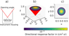 |
Fig. 1. Directional response function of a simple particle telescope. (a): cross-section of a simple particle telescope, where the origin of the normalized coordinate system in panel b is represented by the intersection of the two red lines. (b) and (c): general directional response function of a planar detector to isotropically distributed incident particles within the physical opening cone, which is indicated by the red lines in (a) or by the red cone in (b). The directional response function is given as the color-coded response factor for a spherical grid (black lines) in a coordinate system using normalized axes. |
3. Directional response in μ (cosine of pitch-angle) space
For an isotropic particle flux, the shape of the directional response function of an SEP instrument in μ-space matches the distribution of μ-values of incident particles. However, for a highly non-isotropic particle flux, as observed especially in the early phases of a particle event, the shape of the directional response function in μ-space differs from the distribution of μ-values of incident particles depending on the gradient of the μ-dependent particle flux distribution. By considering the directional response function, it is possible to more realistically consider additional particle trajectories for the approximation of the pitch angle of the particles, that is, the μ-value. This is an improvement over characterizing the pitch angle of the particles based only on the nominal pitch angle, which only takes the center viewing direction of the telescope into account.
Figure 2 shows the process of transforming the directional response function shown in Figs. 1b and c into μ-space for a single selected magnetic field vector in the reference frame of the spacecraft. We note that the natural reference frame of the pitch-angle-dependent particle flux is the solar wind, which is offset to the reference frame of the spacecraft. For relativistic electrons, this offset is small and can therefore be neglected. However, for ion observations, the correct reference frame should be correctly identified thanks to their slower gyration times in comparison to electrons. Panel a of Fig. 2 shows the physical opening cone as the gray cone in a coordinate system using normalized axes. The selected magnetic field vector is located slightly outside the physical opening cone, and is represented by the black arrow in panel a, and by the black dot in panel b. To transform the directional response function to μ-space, we employ the corresponding spherical grid, which is shown in panels b and c of Fig. 1. We obtain a corresponding μ-value for each grid cell by computing the inner product of the vectors pointing from the mid-points of the grid cell to the center of the coordinate system and the selected magnetic field vector, respectively. These μ-values determine the colorized pattern that is visible over the spherical cap of the physical opening cone in the upper panels of Fig. 2. These colors represent the respective μ-bins that are in accordance with the histogram shown in panel c. The heights of the bars are determined by the sum of the directional response factors over the spherical grid cells that are within a specific μ-bin. Due to the finite and directed opening of the telescope, it is only sensitive to part of the μ-space. As the selected magnetic field vector points in the opposite direction of the incoming particle trajectories of the telescope, it responds only to particles with a negative μ-value. The directional response function in μ-space depends on the orientation of the telescope with respect to the magnetic field direction. For a particle telescope with a fixed viewing direction, the μ-response changes according to the magnetic field vector, that is, it is a convolution of Figs. 1b and 2a or alternatively Figs. 1c and 2b.
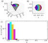 |
Fig. 2. Transforming the directional response function to μ-space. Panel a: physical opening cone (gray cone) of a particle telescope allows incoming particle trajectories originating over a spherical cap of a unit sphere. The top of each trajectory is color coded according to the corresponding μ-value which is determined for the magnetic field vector (black arrow). Panel b: top view of panel a. The black dot indicates the direction of the magnetic field vector. Panel c: The corresponding directional response function in μ (the cosine of the pitch angle) space. |
4. Multiple viewing directions
The determination of the PAD of SEPs requires more than a single telescope on a nonrotating spacecraft. In the following, we discuss the μ-response for a particle instrument consisting of four fixed viewing directions, using a similar setup to SEPT, which consists of two pairs of opposite viewing directions. Part (a) of Fig. 3 shows the center axis of the telescope for the four viewing directions as color-coded arrows. The physical opening cones are indicated in the same colors. For the same selected magnetic field direction (black arrow) as shown in Fig. 2, the μ-response for each telescope – again indicated by the same colors – is shown in the right panel. The dashed colored lines represent the nominal μ-value for each respectively colored viewing direction. As a consequence of the instrument setup, possible particle trajectories are inverse for the blue and green telescopes and for the red and orange telescopes. Hence, the respective μ-response pairs are mirrored at μ = 0.
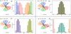 |
Fig. 3. Combined μ-responses of a particle instrument, consisting of four viewing directions for various selected magnetic field vectors. Left panels of (a)–(d): magnetic field vector (black arrow) in relation to the center axis of the four particle telescopes (color-coded arrows). The color-coded cones represent the physical opening cone of each telescope. Right panels of (a)–(d): corresponding μ-response depicted as a color-coded histogram for each telescope. The colored dashed lines represent the respective nominal μ-values. The magnetic field vector is (a) located slightly outside the blue cone, (b) perpendicular to the center axis of each of the four telescopes, (c) located directly in between the blue and red colored center axes, and (d) pointing along the center axis of the red colored telescope. |
Depending on the magnetic field vector changing direction, the μ-responses take on different shapes and cover different parts in μ-space because the telescopes are fixed. Part (b) of Fig. 3 shows the μ-response of the instrument if the magnetic field is perpendicular to the center axis of each of the four telescope. Hence, the μ-responses fully overlap and are all centered around μ = 0. In part (c) of Fig. 3, the responses correspond to a magnetic field vector that is located directly in between the blue and red center axes, resulting in both their responses perfectly overlapping in μ-space. In part (d) of Fig. 3, the responses correspond to a magnetic field vector pointing along the center axis of the red telescope. As a result, the responses of the red and orange telescopes are very narrow and peak at μ = ±1, while the blue and green responses overlap centered around μ = 0. Even though all of the different viewing directions have the same field of view in three-dimensional space, the total range covered in μ-space can vary. Furthermore, depending on the magnetic field vector, the μ-responses of some of the instruments can intersect over part of the μ-space, even though none of the physical opening cones of the telescopes intersect in this way. However, if some telescopes are sensitive to the same part in μ-space, they observe different parts in gyro phase space for particles with constant μ-value.
5. Application of the directional response to an idealized instrument
When measuring the pitch-angle-dependent particle flux with most particle instruments, no detailed information about the incidence angle of the particles for the respective viewing directions is obtained. Instead of obtaining the particle flux for highly resolved μ-bins, a single flux value is measured that corresponds to a larger part of μ-space. For an idealized instrument, that is, with no production of secondary particles and scattering in the instrument housing, the μ-response of the instrument allows us to identify the corresponding parts of μ-space for which a single flux value is observed.
For the case of the μ-response of the instrument shown in part (d) of Fig. 3, the boxes in the upper panel of part (a) of Fig. 4 indicate the corresponding parts of μ-space for which a single flux value can be measured. As the observation of the particle flux is usually measured over some time period, the magnetic field vector does not need to be constant over time and therefore the flux is measured over varying parts of μ-space. If the magnetic field vector fluctuates around its average vector, the μ-response of the instrument can differ significantly depending on whether it is obtained as the averaged response over the fluctuating vectors, or only for the averaged magnetic field vector. The top panel of part (b) of Fig. 4 shows the μ-response of the instrument when the response is averaged over magnetic field vectors that fluctuate around the direction of the selected magnetic field vector shown in part (a) of Fig. 4. In addition to the boxes indicating the parts in μ-space that the respective viewing directions are sensitive to, the top panel shows the magnetic field fluctuation, which is indicated by the black arrow and black circle. In comparison to the μ-response of the instrument obtained for the averaged vector (part (a) of Fig. 4), the responses in part (b) of Fig. 4 are broadened and intersect for a few μ-bins. This demonstrates that more information is preserved if the μ-response of the instrument is determined by the average response over a fluctuating magnetic field vector and not over the averaged magnetic field vector.
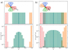 |
Fig. 4. Coverage of a particle instrument in μ-space for a stable magnetic field vector (a) and a fluctuating vector (b). Bottom: colored μ-response for the respectively colored viewing directions of the particle instrument (shown above) corresponding to the stable magnetic field vector shown by the black arrow (same case as part (d) of Fig. 3), or the fluctuating magnetic field vector shown by the black arrow and circle. Top: colored boxes that indicate the parts of μ-space for which the respectively colored viewing directions can obtain a single particle flux value. The colored dashed lines represent the respective nominal μ-values. |
6. Measurement of the pitch-angle-dependent particle flux
The directional response of a particle instrument in μ-space can be used in the forward modeling of SEP transport (e.g., Agueda et al. 2008; Pacheco et al. 2019), where the response is employed to reproduce the measurement process of a gyrotropic PAD of SEPs. If we have precise knowledge about the gyrotropic pitch-angle distribution function, we can determine the expected measurement of the particle instrument with the help of the directional response function that is transformed to μ-space.
The upper panel of Fig. 5 shows the gyrotropic and anisotropic pitch-angle distribution function that we obtained by applying the 1D SEP transport model by Strauss et al. (2017b). The expected particle flux measurement for each viewing direction is obtained by folding the pitch-angle distribution function with the respective μ-response. Due to the measurement process, we lose detailed information about the anisotropic PAD. Furthermore, if some of the μ-responses of the instrument intersect over some part of μ-space, the same part of a gyrotropic PAD contributes to the particle observation of the corresponding viewing directions, but is weighted differently because of the respective responses. As the particle flux observation is affected by the instrument, it is necessary to deconvolve the flux observation and the μ-response of the instrument to determine information about the original PAD of SEPs.
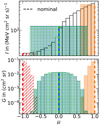 |
Fig. 5. Reproducing the PAD measurement process. Bottom: directional response function in μ-space in accordance with Fig. 4b. Top: by folding an anisotropic PAD of SEPs (black edged histogram) and the μ-response shown in the bottom panel, we can reproduce the measurement of the instrument, which is given by the height of the colored boxes. The colored dashed lines represent the respective nominal μ-values. |
7. Inversion problem for obtaining a distribution of anisotropy values
To improve the quality of observational and modeling studies that apply the anisotropy of SEP observations, we demonstrate a new method for the determination of the anisotropy, that we call ADIM. In contrast to previous anisotropy determination methods, ADIM includes an estimation of uncertainty ranges for the anisotropy. By considering the counting statistics of the observations, we can obtain a distribution of anisotropy values. Using 95% confidence intervals for these distributions, we determine the corresponding uncertainty ranges for the anisotropy.
To obtain information about the anisotropy of the original PAD of SEPs, we apply an inversion process that uses the SEP observation and the μ-response of the instrument. For this inversion process, we use a further simplified version of Eq. (1) from Sullivan (1972) that expresses the determination of the expected coincidence counting rate for a particle telescope. We derive this further simplified version in Appendix A. Thus, we express the expected counting rate of a particle instrument consisting of N telescopes with distinct viewing directions that are at the same location and observe the same differential pitch-angle-dependent particle flux:
In Eq. (2), C(t0) expresses the expected counting rate over some observational period T at time t0 for each of the instrument’s telescopes as a vector. Similarly, Gj represents the μ-response averaged over a fluctuating magnetic field vector for the j-th μ-bin and each viewing direction. M is the number of bins in μ-space. ΔE refers to the absolute range of the observed particle energy. Ij represents the discretized gyrotropic PAD of SEPs and is assumed to be constant over the observational period T of the instrument.
Equation (2) is a classical inversion problem that we can solve for the pitch-angle-dependent particle flux because the counting rates and the μ-response function are known quantities. Due to the generally steep decline of the μ-responses as shown for example in the previous sections, segmenting μ-space into more parts than there are distinctive responses results in an equation system that is underdetermined. Thus, we limit M depending on the number of distinct responses Gj. We refer to the limited number of μ-bins as pixels. As the μ-response of the instrument can vary from one measurement time step to the next, M can take on values from one up to the number of telescopes for a nonrotating SEP instrument, or the number of sectors for a rotating instrument. We choose the width of these pixels according to the shape of the μ-response of the instrument. We discuss how to choose the optimal pixel number and their widths in Appendix B.2.
In principle, by reducing M to less than or equal to the number of telescopes (or sectors), the equation system Eq. (2) can be solved by linear algebra. However, the counting rates C(t0) are a statistical quantity. Thus, we use maximum likelihood optimization to solve Eq. (2) for the particle flux Ij. Again, we discuss details in Appendix B.3. Once the particle flux is obtained, the anisotropy can be computed by applying the discrete representation of Eq. (1). As most particle instruments only provide the particle flux for an observational period as a single value, we consider the counting statistics of the observation to generate a distribution of anisotropy values. Therefore, we not only consider the result of the optimization that best replicates the observation, but also the results that yield re-determined counting rates that are within the respective counting statistics of the observation. For measurement time-steps where no sufficient statistics (i.e., < 100 anisotropy values) are obtained, we do not determine an anisotropy or the uncertainty of the anisotropy. If ADIM yields ≥100 anisotropy values, we characterize the anisotropy by the median of the anisotropy distribution. To reflect the fact that the outline shape of the distribution need not to be symmetrical, we choose to quantify the uncertainty on the anisotropy through confidence intervals based on percentiles, using a 95% confidence level. We demonstrate a first-principle validity check of ADIM using in situ magnetic field data and synthetic PAD data in Appendix C.
To apply ADIM to observational SEP data, the following assumptions and limitations are required: we assume that (1) we are dealing with an ideal detector that only detects one specific particle species within a specific finite energy range (i.e., we neglect the detection of other particle species and higher energetic particles); (2) the particle flux is constant over the accumulation time of the instrument; (3) the particle flux is gyrotropic; and that (4) the correct reference frame of the magnetic field vector is identified.
8. Application to the Solar Electron and Proton Telescope on board STEREO
Figure 6 shows the final result of ADIM for a solar electron event observed by SEPT on board STEREO B in the range of 65–105 keV on 14 August in 2010, which has been modeled by Dröge et al. (2016). For the differential directional particle flux I, we used level 2 SEPT data1 that have a time resolution of ∼60 s, which is set by the measurement time-steps of the instrument. We estimated corresponding uncertainty ranges for the flux data by utilizing the counting statistics of the measurement. For the μ determination, we used 8 Hz STEREO/MAG (Acuña et al. 2008) data2, and the response of the electron detector of the SEPT. We simulated this response with the help of the GEANT4 toolkit (Agostinelli et al. 2003) and demonstrate the simulation results in Appendix B.1. The nominal μ-values are determined for a one-minute averaged magnetic field, and the μ-response is averaged over the fluctuating in situ magnetic field. Both the nominal μ-values and μ-response are determined for the respective measurement time-steps of SEPT. The variations of the nominal μ-values are due to changes in the magnetic field direction. In the background phase (9:00 to ∼10:30 UTC), the particle flux is roughly constant for all viewing directions and is independent of the respective μ-coverage which varies moderately over this time-period.
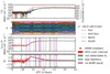 |
Fig. 6. ADIM data product for the omnidirectional particle flux and anisotropy for a solar electron event observed by SEPT on board STEREO B on 14 August, 2010. From top to bottom: differential directional particle flux including estimated uncertainty ranges as shaded areas that are barely visible because of the large extent of the logarithmic y-axis, nominal μ-value (solid lines) and extent of μ-response (shaded area), omnidirectional particle flux, and anisotropy. In the panels for the omnidirectional flux and anisotropy, the black dots represent the median value of the respective distributions determined by ADIM. The red bars indicate the corresponding uncertainty ranges that are obtained by applying 95% confidence intervals. The green and purple bars mark time-periods where ADIM did not yield a result (we give further details in Sect. 8). The gray shaded areas in the anisotropy panel indicate anisotropy values which cannot be obtained by ADIM. |
Around 10:30 UTC, the particle flux first starts to increase for the Sun viewing direction, while the particle flux for the anti-Sun, North, and South telescopes increases between approximately 10:40 and 10:50 UTC. As a consequence of the much higher particle flux for the Sun viewing direction with respect to the other viewing directions and the generally stable μ-coverage for the Sun viewing direction (μ ≈ 1), a positive anisotropy is seen from 10:30 to 15:00 UTC.
The bottom panel of Fig. 6 shows the results of ADIM for the determination of the anisotropy A1. Similar to the uncertainty estimation of the anisotropy, ADIM can be used to yield the omnidirectional particle flux, including a corresponding uncertainty estimation. The final results for the omnidirectional particle flux Iomni are shown in the second panel from the bottom. For each accumulation period of STEREO/SEPT, the median values of the distribution of the anisotropy and the omnidirectional particle flux are shown as black dots. The red bars represent the estimated uncertainty ranges by applying 95% confidence intervals.
The gray shaded area marks the anisotropy values that cannot be obtained by ADIM. As STEREO/SEPT only provides SEP measurements for four viewing directions, the number of pixels is limited in the application of ADIM. As a consequence, the highest obtainable anisotropy value is limited as well. In cases of weak pitch-angle scattering conditions, the anisotropy of the original PAD of SEPs might be underestimated. To increase the highest obtainable absolute anisotropy value, we cannot increase the number of pixels in the application of ADIM, because this would lead to an underdetermined equation system. Instead, to accommodate for the uncertainty introduced due to the limitation of the SEPT, we use ADIM for pixel widths that are slightly varied by ±0.1. We note that smaller variations of the pixel width are only applicable if the μ-responses do not show fluctuations due to an overly fine binning. In contrast, larger variations of the pixel width are not applicable either, because the particle flux levels determined by ADIM mostly fail to replicate the observation.
In addition, we flag the measurement time-steps that result in no determination of the anisotropy: “bad coverage” is where all μ-responses intersect in the center of μ-space, which is not the case for the SEP event shown in Fig. 6; “bad statistics”, where some of the μ-responses of the instrument almost fully intersect, but the respective counting statistics do not agree; and “no ADIM result”, where ADIM fails to obtain sufficient statistics, because the gradient of the PAD of SEPs cannot be reasonably estimated due to the coverage of the μ-response of the instrument, as specifically the restriction to too few viewing directions. These scenarios are marked for measurement time-steps by blue, green, and purple bars, respectively.
In the pre-event phase (9:00 to ∼10:30 UTC) the median values of the one-minute anisotropy distributions show large fluctuations. A few values are even larger than 1 or smaller than −1, respectively. For these larger absolute anisotropy values, the corresponding uncertainty ranges are on the order of ±0.5 up to ±0.7, which is mostly due to the low particle flux or count rates. Beginning with the increase in the particle flux for the Sun viewing direction (∼10:30 UTC), the uncertainty of the anisotropy becomes smaller because of the considerable increase in counting statistics. Shortly before 10:50 UTC, the anisotropy shows a local minimum which is a consequence of the drastic increase in the particle flux of the south viewing direction and a decrease in the particle flux of the north viewing direction due to a change in the μ-coverage. The anisotropy reaches its peak at 10:47 UTC with a maximum value of A1 = 1.90 and an uncertainty on the order of ΔA1 ≈ ±0.1. In the decreasing phase of the anisotropy from ∼10:50 to 15:00 UTC, the uncertainty on the anisotropy stays on the order of ±0.1. For this specific event, the uncertainty ranges of the anisotropy (red bars) are far from the highest (lowest) possible obtainable anisotropy value (gray areas), which indicates that we do not underestimate the anisotropy. We compare the results obtained by ADIM to those obtained using other anisotropy determination methods for the same event in Appendix D.
9. Summary and conclusion
In this work, we present a new method for determining the anisotropy of SEPs that will help to improve their interpretation. In addition to previous anisotropy determination methods, our new method includes an estimation of uncertainty ranges. We estimate these uncertainty ranges by determining a distribution of anisotropy values and applying 95% confidence intervals. Hence, we refer to our new method as the anisotropy distribution inversion method (ADIM). We generate a distribution of anisotropy values by considering the counting statistics of the measurements, because particle instruments only provide one particle flux value per viewing direction per accumulation time-period.
To further improve on previous anisotropy determination methods, we not only approximate the pitch angle of the particles by the nominal pitch angle, which is defined by the time-averaged magnetic field and the center axis of the respective telescope, but also take into account that a particle telescope is sensitive to a range of particle pitch angles. Therefore, we introduce the directional response function of a particle instrument and demonstrate how to transform it into μ (cosine of the pitch angle) space. As the μ-response of an instrument changes with the direction of the magnetic field, we can easily consider the variability of the magnetic field by averaging the μ-response over the accumulation time of the instrument.
We apply the μ-response of the instrument to invert the SEP measurements to infer information about the anisotropy of the original PAD of the SEPs. We solve this inversion problem by maximum likelihood optimization. To obtain a distribution of anisotropy values, we consider all solutions of one optimization run that are in good agreement with the counting statistics of the observation. For each of these solutions, an anisotropy value can be computed. If there is a sufficient number of anisotropy values, we estimate the uncertainty on the anisotropy by 95% confidence intervals based on percentiles.
Including the uncertainty on the anisotropy in future SEP studies will not only enhance the quality of observational investigations, but will also create new opportunities for transport modeling studies. By constraining the models with the new uncertainties, the validity range of different model runs can be mathematically determined and even uncertainties on the model parameters such as the mean free path can be derived. In principle, our new method for determining a distribution of anisotropy values can be applied to any other particle instrument, but requires the instrument’s directional response. In our case, the response function of the instrument is determined with the help of a GEANT4 simulation which we demonstrate in Appendix B.1. In this work, we applied ADIM to the electron detector of the STEREO/SEPT instrument. Therefore, applying ADIM to the Electron and Proton Telescope (EPT) on board Solar Orbiter is especially straightforward due to the similarity with the SEPT instrument. Furthermore, we note that the directional response function of the SEPT transformed to μ-space allows us to employ forward transport modeling by using the modeling approach by Agueda et al. (2008).
We demonstrate the final results of ADIM for a solar electron event on the 14 August 2010 that was observed by the SEPT instrument on board STEREO B. For this specific event, we obtain uncertainties on the anisotropy on the order of ±0.1. By applying ADIM, we can clearly identify whether the increase in the anisotropy deviates significantly from zero, which could not be achieved by previous anisotropy determination methods. In the pre-event phase of this event, we find that the uncertainty on the anisotropy is mostly on the order of ±0.5 that is attributable to the low particle flux or counting statistics. The median values of the determined anisotropy distributions show larger fluctuations, indicating that it is not meaningful to determine the anisotropy for such periods. With the increase in the particle flux or counting statistics, the uncertainty on the anisotropy gets smaller and can therefore be separable from zero. In a few cases, we find that ADIM applied to STEREO/SEPT observations does not allow us to determine the anisotropy or its uncertainty for observational time-periods for one of the following reasons: (a) The combined μ-responses of the telescopes overlap in the center of μ-space (μ = 0) and therefore cannot perform a meaningful inversion. (b) Two μ-responses cover mostly the same part of μ-space, and therefore we expect their measurements to be about the same. However, if the estimated uncertainty ranges of these measurements do not intersect, we cannot perform an inversion following the rules described in this work. (c) The ADIM does not yield sufficient statistics for the determination of uncertainty ranges, which can mostly be attributed to the STEREO/SEPT providing only four-sector measurements. Furthermore, as a consequence of the aforementioned limitation of the SEPT, the highest detectable anisotropy value that can be obtained by ADIM is limited. We identify whether the anisotropy is potentially underestimated if the determined uncertainty range of the anisotropy comes close to the highest obtainable anisotropy value.
Acknowledgments
We acknowledge financial support by the Deutsche Forschungsgemeinschaft (DFG) via project GI 1352/1-1. The STEREO/SEPT project is supported under grant 50OC2102 by the Federal Ministry of Economics and Technology on the basis of a decision by the German Bundestag. This work was performed in the framework of the SERPENTINE project, which has received funding from the European Union’s Horizon 2020 research and innovation program under grant agreement No. 101004159. N.D. is grateful for support by the Turku Collegium for Science, Medicine and Technology of the University of Turku, Finland.
References
- Acuña, M. H., Curtis, D., Scheifele, J. L., et al. 2008, Space Sci. Rev., 136, 203 [Google Scholar]
- Agostinelli, S., Allison, J., Amako, K., et al. 2003, Nucl. Instrum. Methods Phys. Res. A, 506, 250 [Google Scholar]
- Agueda, N., & Lario, D. 2016, ApJ, 829, 131 [NASA ADS] [CrossRef] [Google Scholar]
- Agueda, N., Vainio, R., Lario, D., & Sanahuja, B. 2008, ApJ, 675, 1601 [NASA ADS] [CrossRef] [Google Scholar]
- Brüdern, M., Dresing, N., Heber, B., et al. 2018, Cent. Eur. astrophys. bull., 42, 2 [Google Scholar]
- Carcaboso, F., Gómez-Herrero, R., Espinosa Lara, F., et al. 2020, A&A, 635, A79 [NASA ADS] [CrossRef] [EDP Sciences] [Google Scholar]
- Dresing, N., Gómez-Herrero, R., Heber, B., et al. 2014, A&A, 567, A27 [NASA ADS] [CrossRef] [EDP Sciences] [Google Scholar]
- Dröge, W., Kartavykh, Y. Y., Dresing, N., Heber, B., & Klassen, A. 2014, J. Geophys. Res. (Space Phys.), 119, 6074 [CrossRef] [Google Scholar]
- Dröge, W., Kartavykh, Y. Y., Dresing, N., & Klassen, A. 2016, ApJ, 826, 134 [Google Scholar]
- Gómez-Herrero, R., Dresing, N., Klassen, A., et al. 2015, ApJ, 799, 55 [Google Scholar]
- Lario, D., Raouafi, N. E., Kwon, R.-Y., et al. 2014, ApJ, 797, 8 [NASA ADS] [CrossRef] [Google Scholar]
- Müller-Mellin, R., Gomez-Herrero, R., Böttcher, S., et al. 2008, Int. Cosmic Ray Conf., 1, 371 [NASA ADS] [Google Scholar]
- Pacheco, D., Agueda, N., Aran, A., Heber, B., & Lario, D. 2019, A&A, 624, A3 [NASA ADS] [CrossRef] [EDP Sciences] [Google Scholar]
- Strauss, R. D. T., Dresing, N., & Engelbrecht, N. E. 2017a, ApJ, 837, 43 [NASA ADS] [CrossRef] [Google Scholar]
- Strauss, R. D., Ogunjobi, O., Moraal, H., McCracken, K. G., & Caballero-Lopez, R. A. 2017b, Sol. Phys., 292, 51 [NASA ADS] [CrossRef] [Google Scholar]
- Sullivan, J. D. 1972, Nucl. Instrum. Methods, 98, 187 [CrossRef] [Google Scholar]
- Thomas, G. R., & Willis, D. M. 1972, J. Phys. E Sci. Instrum., 5, 260 [NASA ADS] [CrossRef] [Google Scholar]
- van den Berg, J., Strauss, D. T., & Effenberger, F. 2020, Space Sci. Rev., 216, 146 [NASA ADS] [CrossRef] [Google Scholar]
Appendix A: General inversion problem
For our new method to determine the anisotropy of SEPs, we use an inversion process to infer information about the anisotropy of the original PAD of SEPs. In the following, we give a detailed derivation of this inversion problem. We begin with Eq. (1) from Sullivan (1972), which describes the determination of the expected coincidence counting rate of a single particle telescope. This latter depends on the original PAD of SEPs and the directional response of the telescope. In Sullivan (1972), the expected coincidence counting rate C(x, t0) between the opening of the telescope and its planar detector (or a stack of planar detectors) is expressed as:
In Eq. (A.1), the coincidence counting rate C(x, t0) is obtained by the product of the detection efficiency ϵα and the differential directional particle flux Jα(E, ω, x, t), which is summed over the α-th species of particle and integrated over energy E, the full-sphere solid angle Ω, the surface area of the detector S, and the accumulation time of the telescope T. In this formula, x labels the spatial coordinates of the telescope, t0 the starting time of the observation, dt the time integration, dσ an element of the surface area of the last detector,  the unit vector in direction of ω, dω an element of the solid angle, dE the energy integration, and t the time. In the same manner as Sullivan (1972) we assume that dσ, ω, and x are independent of time, that no transformation of particle type occurs, that the particle trajectory in the instrument is a straight line, that Jα is independent of x as well as σ, and that ϵα is independent of t as well as x. Most SEPs are relativistic particles. Due to their high velocities, the gyro motion of such particles is negligible for traveling the usually very short distances from the opening of the telescope to the detector. Furthermore, we consider an ideal telescope where ϵα = 0 for any other particle species other than for example electrons. By dropping the subscript α, and defining the directional detector response function A(E, ω) as
we can simplify Eq. (A.1) to:
Equation (A.3) expresses the expected counting rate for a single telescope. As we assume that Jα is independent of x, we can drop the dependency of the expected counting rate C on x. To express the expected counting rate for a particle instrument consisting of N telescopes with distinct viewing directions that are at the same location in space and observe the same differential directional particle flux we vectorize Eq. (A.3):
Equation (A.4) is a classical inversion problem which allows to obtain the differential directional particle flux J(E, ω, t) by, e.g., minimizing the combined expected counting rate vector C(t0) with respect to the observation Cobs(t0). Once the particle flux is obtained, an anisotropy value can be computed by applying Eq. (1). However, this equation system is underdetermined and to apply it for example to STEREO/SEPT observations we have to make further simplifications.
A.1. Simplifying the inversion problem
In the following, we further constrain Eq. (A.4) by assuming that the particle flux J(E, ω, t) is gyrotropic3 in μ-space. Therefore, we express J(E, ω, t) in μ-space instead of the spherical coordinate system of the instrument, e.g., spacecraft coordinates. We assume that all particles propagate along a magnetic field B, and that their spatial distribution depends on the gyro phase φ, and the cosine of the pitch angle  , where r represents the trajectory of the particles. For a spherical coordinate system where the z-axis is aligned with the direction of the magnetic field
  , the gyro phase φ represents the azimuth angle, and μ represents the cosine of the zenith angle θ. Thus, we can rotate any vector
  , where
  ,
,  , and
, and  represent the unit vectors of the coordinate system of the instrument and
  ,
,  , and
, and  represent the respective coordinates to a corresponding vector
  , where
  ,
,  , and
, and  represent the unit vectors of the
  aligned coordinate system and ar, bφ, and cθ represent the respective coordinates.
In Eq. (A.5), R(B(t)) labels the rotation matrix that aligns the z-axis of the instrument’s coordinate system to the direction of the magnetic field  . As this rotation indirectly depends on time due to the magnetic field vector, a dependency on time is introduced to the directional response function in μ-space A(E, φ, μ, t). By furthermore assuming that the differential directional particle flux J(E, φ, μ, t) is gyrotropic, i.e., does not depend on the gyro phase φ, Eq. (A.4) can be expressed in the magnetic-field-aligned spherical coordinate system:
To further simplify the equation system Eq. (A.6), we neglect the contribution of particles that have energies not within a specific energy range [E0,E1], i.e., we assume that the detector response function A(E, φ, μ, t) = 0 for particles with energies ranging [0,E0) or (E1,∞]. Within this specific energy range [E0,E1], we assume that neither the differential directional particle flux J(E, μ, t) nor the response function A(E, φ, μ, t) changes with energy. Thus, the energy integration simplifies:
In Eq. (A.7), ΔE is given by ΔE = E1 − E0. Furthermore, we discretize the μ integration by partitioning μ-space into a number of Mμ-ranges [μj,μj + 1], where j can take on values from 0 to M − 1. We assume that J(μ, t) is constant within each of the individual μ-ranges, but can take on different values for each range, respectively. In the following, the discretized differential directional particle flux for the j-th μ-range is labeled as Ij(t). Thus, the spherical integration simplifies:
We define the combined directional detector response factor Gj(t) for the j-th μ-range:
In Eq. (A.9), Gj(t) is given for one specific magnetic field vector B(t) because the latter determines the rotation from the spherical coordinate system of the instrument to μ-space. Furthermore, we approximate the time integration by discretizing it as follows..:
where the accumulation duration T is partitioned into Nt equal time ranges Δt so that T = Nt × Δt. The fully discretized equation system of Eq. (A.6) is expressed:
In Eq. (A.11), Gj, i and Ij, i represent the directional detector response factor and differential directional particle flux for the i-th time range of the accumulation duration and the j-th μ-range, respectively. Finally, we have to assume that the differential directional particle flux Ij, i remains constant within the accumulation period of the instrument and thus drop the subscript i. By defining the time-averaged directional response factor  as
as
we can express the discretized equation system as follows:
This final discretized equation system Eq. (A.13) can be solved for the μ-dependent particle flux Ij, if the directional response function of the instrument in μ-space Gj is known, because C(t0) is given by the observation of a SEP instrument. Thus, Eq. (A.13) can be applied to infer information about the anisotropy of the μ-dependent SEP flux. This final discretized equation system Eq. (A.13) can be applied to most SEP instruments, even for rotating ones, if none of the following assumptions and limitations are violated: (1) An ideal detector that only detects one specific particle species within a specific finite energy range (i.e., we neglect the detection of other particle species and of higher energetic particles), (2) the particle flux is constant over the accumulation time of the instrument, (3) the particle flux is gyrotropic, and (4) the correct reference frame of the magnetic field vector is identified. The application of this inversion problem requires the directional response function of the SEP instrument, which could for example be obtained by a GEANT4 (Agostinelli et al. 2003) simulation.
Appendix B: Implementation details of ADIM for STEREO/SEPT observations
In the following, we describe our new determination method for the anisotropy of SEP observations by the STEREO/SEPT instrument, using the inversion problem given by Eq. (A.13). By considering the counting statistics in the inversion problem, we can generate a distribution of anisotropy values. The distribution of anisotropy values allows us to estimate the corresponding uncertainty ranges for the anisotropy. To apply this inversion problem, the directional response function of STEREO/SEPT is required. In Sect. B.1 we describe the determination process of the directional response function of STEREO/SEPT. In Sect. B.2 we describe further details of the implementation of ADIM to SEP observations by STEREO/SEPT.
B.1. The directional response function of STEREO/SEPT
We obtain the directional response to electrons in the nominal energy range of 65–105 keV of the SEPT instrument by running a GEANT4 (Agostinelli et al. 2003) simulation. As all four electron (i.e., foil-side) telescopes of the SEPT instrument are built equally, we only simulated the response for one of the telescopes. In this response simulation of a single electron telescope, we neglect the contribution of ions and higher energetic electrons. In more detail, we distribute the starting points of incoming electrons isotropically over a full sphere and perform this simulation for incoming electrons with primary energy ranges matching the electron bins of the SEPT detector that are defined in Table 12 of (Müller-Mellin et al. 2008). We determine the directional response factors by Monte-Carlo integration, as described in Sullivan (1972). Each response factor is determined for a spherical segment. These spherical segments are defined by cutting the sphere by a pair of parallel planes at specific zenith angles. As a result of our simulation, we find that the detector does not respond to electrons with initial energies up to 125 keV that are coming from opposed to the nominal viewing direction. Furthermore, we find that the response for electrons coming from the side is several magnitudes smaller compared to the highest response, which is found closest to the center axis of the telescope. In the application of ADIM, we do not employ the full sphere simulation or the response simulation limited to the physical opening cone of the detector, which is shown in Fig. 1. Instead, we simulate the angular response up to ±45° around the center axis of the telescope as a compromise for the fact that the detector can respond to particles from outside the telescope’s physical opening, and to easily increase the statistics of the response simulation. In contrast to Fig. 1, we consider that the response can be extended over the limitation of the physical opening cone as a consequence of physical processes such as scattering and/or the production of secondary particles within the housing of the instrument or in the foil that is located in front of the electron detector.
Figure B.1 shows the directional response of one foil-side detector of the STEREO/SEPT instrument to electrons with an initial energy of between 65 and 105 keV as a result of our GEANT4 simulation in a coordinate system using normalized axes. Panel (a) of this figure shows a simplified cross-section of the SEPT telescope, where the origin of the normalized coordinate system in panel (b) is represented by the intersection of the two lines that connect the detector’s edges to the edges of the physical opening. Panels (b) and (c) of Fig. B.1 show the color-coded directional detector response factors for a spherical grid (black lines) that consists of 1267 grid cells from the side and top, respectively. The physical opening cone is represented by the red cone in panel (b) and the red circle in panel (c). The directional response extends over the limitation of the physical opening cone, clearly indicating that particles with incident angles out of the physical opening cone can contribute to the response of the detector. This extension over the boundary of the physical opening cone is rather due to scattering in the instrument’s housing or foil and not due to the production of secondary particles, because the electron energies are still quite low. The maximum of the directional response is found around the center axis of the telescope. With increasing zenith angle, the response decreases drastically from its maximum value, as highlighted by the logarithmic axis for the color coded directional response factor. To obtain the directional response in μ-space, we further segment the directional response factors that are obtained for the zenith angle segmentation by partitioning each zenith angle segment for the azimuth angle. This spherical grid of 1267 grid cells over the ±45° spherical cap is indicated by the black lines in panels (b) and (c) of Fig. B.1. All spherical grid cells measure the same solid angle which is achieved by a nonequidistant grid for the zenith angle, where the equidistant segmentation of the azimuth angle increases with increasing zenith angle. Similarly, as described in Sects. 3 and 4, we obtain the combined directional response function of the STEREO/SEPT instrument in μ-space.
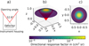 |
Fig. B.1. Directional electron response function of SEPT. (a): Simplified cross-section of the SEPT telescope, where the origin of the normalized coordinate system in panel (b) is represented by the intersection of the two lines that connect the detector’s edges to the edges of the physical opening. (b) and (c): Directional response of one of the electron telescopes of STEREO/SEPT to isotropically distributed incident electrons with primary energy between 65 and 105 keV in a coordinate system using normalized axes. The response extends over the physical opening cone of the instrument, which is indicated by the red lines in (a), the red cone in (b), or the red circle in (c). The black lines in (b) and (c) represent the spherical grid for which the directional response factors are given. |
B.2. Choosing the pixel number and width for the inversion process
In the following, we describe the application of the general inversion problem Eq. (A.13) to SEP observations by the STEREO/SEPT instrument in more detail. To solve the equation system Eq. (A.13) for the discretized particle flux the number of μ-bins M has to be limited, because the STEREO/SEPT instrument only provides four-sector measurements. Therefore, for STEREO/SEPT observations, we segment the μ-space into either one, two, three, or four μ-bins depending on the shape of the combined μ-response of the instrument for each 60-second accumulation period. We refer to these μ-bins as pixels. Selecting a larger number of pixels than there are distinct responses leads to an underdetermined equation system.
Figure B.2 shows an example for the estimation of the optimal pixel number and width for the combined μ-response of the STEREO/SEPT instrument that is shown in the bottom panel. We automated the determination of the number of distinct responses, i.e., the number of pixels in the inversion, by utilizing the full width at half maximum (FWHM) of the respone of each telescope. We define two neighboring responses as distinct if the highest response factors are not within the FWHM of the adjacent response, respectively. In cases where there are three or four distinct responses, we estimate the optimal widths of each pixel by varying the widths in steps of 0.1 in μ-space systematically. For each step of the variation, we determine the total directional response factor of each viewing direction within each pixel. For the j-th pixel, we obtain the highest response factor  of any viewing direction, where n labels any of the four viewing directions. We then estimate the optimal pixel width by maximizing the sum of the highest response factor over each pixel
  . The top of Fig. B.2 shows the optimal number of pixels and widths for the combined responses shown directly underneath. Here, the color coding of each pixel represents the color matching to the viewing direction with the highest response factor.
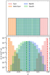 |
Fig. B.2. Example of optimal pixel number for ADIM. Bottom: Combined μ-responses of STEREO/SEPT that shows three distinctive responses, which are obtained by averaging the responses over a fluctuating magnetic field vector for the measurement time-step centered at 11:34 UTC on 14 August 2010. Top: Corresponding number and width of pixels (μ-bins) for the utilization of ADIM. |
The determination of the pixel number and width is straightforward if the instrument’s μ-response only shows one or two distinct responses. In the case of only two distinctive μ-responses, i.e., there are two overlapping responses in each μ-hemisphere, we separate the μ-space in two halves. In cases where there is only one pixel, i.e., the four responses overlap centered around μ = 0, no information about the anisotropy can reliably be obtained, because all viewing directions are sensitive to the same part of a PAD of SEPs. By restricting M to either M = 2, M = 3, or M = 4 in the equation system of Eq. (A.13), we can solve it for the discretized μ-dependent particle flux Ij and infer information on the original PAD of SEPs.
B.3. Estimating a particle flux level for each pixel
For the STEREO/SEPT instrument, we solve the inversion problem Eq. (A.13) for either two, three, or four pixels (bins in μ-space). As the observed counting rates come from a statistical universe, we use maximum likelihood optimization for solving the equation system. Therefore, we aim to minimize
where n refers to the different telescopes, Cn, obs to the observed counting rate, Cn, inv to the re-determined counting rate obtained by Eq. (A.13), and ΔCn, obs the uncertainty of the observation that is due to the counting statistics. We perform successive optimization runs to obtain the flux levels that replicate the observations best. In one optimization run, we tabularize ten particle flux levels within each pixel and compute χ2 for each combination. The combination that minimizes χ2 determines ten new flux levels within each pixel for a successive optimization run. For each pixel, we equidistantly space ten new flux levels over the range obtained by varying the respective flux level that minimizes χ2 by ±25%. We begin our optimization with the same flux levels tabulation for each pixel: 1, 5, 10, 50, 100, 500, 1000, 5000, 10000, and 50000 (MeV cm2 sr s)−1. We allow a maximum of 50 successive optimization runs, which we stop if the corresponding χ2 of two successive runs no longer significantly reduces.
Appendix C: First-principle validity check of the Anisotropy Distribution Inversion Method
As a means to validate our new method to determine a distribution of anisotropy values and thus corresponding uncertainty ranges, we generated synthetic PAD data through transport modeling4 (Strauss et al. 2017b; van den Berg et al. 2020). By applying in situ magnetic field data and using Eq. (A.11) we reduce these synthetic PADs to pitch-angle coverage cases of STEREO/SEPT. We apply ADIM to these hybrid PAD observations and determine the anisotropy. As the anisotropy of the synthetic PADs is well known, we can carry out a meaningful comparison to the anisotropy values obtained by ADIM.
Figure C.1 shows a validity check of ADIM where we kept the original PAD of SEPs for the determination of the hybrid observation constant over time. We generated a synthetic PAD with well-known anisotropy value (A1 = 2.0) where we selected δ-injection and a radial mean free path of λr = 0.73AU. For the determination of the μ-response that is averaged over the fluctuating in situ magnetic field within the respective measurement time steps of the instrument we use 8Hz STEREO/MAG data5, measured on STEREO B on 7 November in 2013 from 13:00 to 15:00 UTC. The upper panel of Fig. C.1 shows the reduced PADs. The second panel shows the nominal μ-values as colored solid lines, and the extent of the averaged μ-responses as shaded areas. The two bottom panels show the azimuth (φ) and the zenith angle (θ) variation of the in situ magnetic field (RTN coordinates). The panel in the middle shows the comparison of the well-known anisotropy value of the synthetic PAD (black circles) with the results of ADIM (black dots and red bars), and in addition to the discretized anisotropy determination method (Brüdern et al. 2018) (blue crosses), taking into account the full cone opening angle (fcoa). Periods for which ADIM did not yield any results are marked by the blue, green and purple shaded areas. The gray shaded areas mark anisotropy values that can not be obtained by ADIM, due to the limitation of four viewing directions of the STEREO/SEPT instrument. The comparison clearly shows that our new method is an improvement for the determination of the anisotropy, because the results of ADIM are much less dependent on the pitch-angle coverage than it is the case for the results of the previous determination method. Furthermore, this comparison indicates that the determination of the anisotropy utilizing ADIM should be understood as a lower boundary for original anisotropy of a PAD of SEPs.
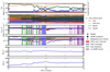 |
Fig. C.1. First-principle validity check of ADIM. From top to bottom, hybrid particle flux observation, nominal μ-value (solid lines) and extent of averaged μ-response (shaded area), anisotropy determination comparison, azimuth and zenith angle of the in situ magnetic field vector (RTN coordinates). In the anisotropy panel, the black dots and red bars represent the result of ADIM applied to the hybrid observation, the black circles represent the well-known anisotropy value of a synthetic PAD, and the blue crosses represent the anisotropy obtained by a previous anisotropy determination method. The green, blue, and purple bars mark time periods where ADIM did not yield a result. The gray shaded areas in the anisotropy panel indicate anisotropy values which cannot be obtained by ADIM. |
Appendix D: Comparison with previous anisotropy determination methods
Figure D.1 shows a comparison of the final result of ADIM with previous anisotropy determination methods for the same solar electron event as shown in Fig. 6. Both of the upper panels are the same as in Fig. 6, which are discussed in Sect. 8.
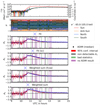 |
Fig. D.1. Comparison of ADIM results to previous determination methods of the anisotropy for a solar electron event observed by SEPT on board STEREO B on 14 August 2010. From top to bottom, differential directional particle flux, nominal μ-value (solid lines) and extent of μ-response (shaded area). Each of the four bottom panels shows the respective comparison to one of the previously used determination methods of the anisotropy (blue circles) to the results of ADIM (black dots and red bars). The previous determination methods are: "Fit", "Fit (sc)", "Weighted sum", and "Weighted sum (fcoa)", as explained in the text. |
The following panels show the comparison of ADIM (median as black dots and uncertainty range as red bars) to one of the previously used determination methods of the anisotropy (blue circles). The previous determination methods are: "Fit" where the observed particle flux is fitted over the nominal μ-values by a truncated Legendre polynomial (e.g., Agueda & Lario 2016; Carcaboso et al. 2020), "Fit (sc)" which is the same as ("Fit"), but in addition assumes that the PAD of SEPs is always a beam as a stability criterion (sc, Dröge et al. 2014), "Weighted sum" which is a discrete interpretation of the integral definition of A1 (Brüdern et al. 2018), "Weighted sum (fcoa)"which is the same as "Weighted sum", but in addition uses the telescope’s full cone opening angle (fcoa) in μ-space as a weight (Brüdern et al. 2018).
Both "Fit" and "Fit (sc)" show smaller values for the anisotropy than ADIM around the maximum for the anisotropy (∼ 10:50 UTC). Likewise, as a consequence of going from three to four distinct nominal μ-values from ∼11:00 to ∼11:50 UTC, the anisotropy values of "Fit" and "Fit (sc)" are larger than the anisotropy obtained by ADIM. For the same time period and reason, "Weighted sum" shows even larger anisotropy values than the ones obtained by ADIM. The anisotropy values obtained using the "Weighted sum (fcoa)" method are in good agreement with the results of ADIM around ∼ 10:50 UTC. For the declining phase of the anisotropy (∼11:00 to ∼11:50 UTC) the anisotropy values obtained by "Weighted sum (fcoa)" are slightly below the ones of ADIM.
All Figures
|
Fig. 1. Directional response function of a simple particle telescope. (a): cross-section of a simple particle telescope, where the origin of the normalized coordinate system in panel b is represented by the intersection of the two red lines. (b) and (c): general directional response function of a planar detector to isotropically distributed incident particles within the physical opening cone, which is indicated by the red lines in (a) or by the red cone in (b). The directional response function is given as the color-coded response factor for a spherical grid (black lines) in a coordinate system using normalized axes. |
| In the text | |
|
Fig. 2. Transforming the directional response function to μ-space. Panel a: physical opening cone (gray cone) of a particle telescope allows incoming particle trajectories originating over a spherical cap of a unit sphere. The top of each trajectory is color coded according to the corresponding μ-value which is determined for the magnetic field vector (black arrow). Panel b: top view of panel a. The black dot indicates the direction of the magnetic field vector. Panel c: The corresponding directional response function in μ (the cosine of the pitch angle) space. |
| In the text | |
|
Fig. 3. Combined μ-responses of a particle instrument, consisting of four viewing directions for various selected magnetic field vectors. Left panels of (a)–(d): magnetic field vector (black arrow) in relation to the center axis of the four particle telescopes (color-coded arrows). The color-coded cones represent the physical opening cone of each telescope. Right panels of (a)–(d): corresponding μ-response depicted as a color-coded histogram for each telescope. The colored dashed lines represent the respective nominal μ-values. The magnetic field vector is (a) located slightly outside the blue cone, (b) perpendicular to the center axis of each of the four telescopes, (c) located directly in between the blue and red colored center axes, and (d) pointing along the center axis of the red colored telescope. |
| In the text | |
|
Fig. 4. Coverage of a particle instrument in μ-space for a stable magnetic field vector (a) and a fluctuating vector (b). Bottom: colored μ-response for the respectively colored viewing directions of the particle instrument (shown above) corresponding to the stable magnetic field vector shown by the black arrow (same case as part (d) of Fig. 3), or the fluctuating magnetic field vector shown by the black arrow and circle. Top: colored boxes that indicate the parts of μ-space for which the respectively colored viewing directions can obtain a single particle flux value. The colored dashed lines represent the respective nominal μ-values. |
| In the text | |
|
Fig. 5. Reproducing the PAD measurement process. Bottom: directional response function in μ-space in accordance with Fig. 4b. Top: by folding an anisotropic PAD of SEPs (black edged histogram) and the μ-response shown in the bottom panel, we can reproduce the measurement of the instrument, which is given by the height of the colored boxes. The colored dashed lines represent the respective nominal μ-values. |
| In the text | |
|
Fig. 6. ADIM data product for the omnidirectional particle flux and anisotropy for a solar electron event observed by SEPT on board STEREO B on 14 August, 2010. From top to bottom: differential directional particle flux including estimated uncertainty ranges as shaded areas that are barely visible because of the large extent of the logarithmic y-axis, nominal μ-value (solid lines) and extent of μ-response (shaded area), omnidirectional particle flux, and anisotropy. In the panels for the omnidirectional flux and anisotropy, the black dots represent the median value of the respective distributions determined by ADIM. The red bars indicate the corresponding uncertainty ranges that are obtained by applying 95% confidence intervals. The green and purple bars mark time-periods where ADIM did not yield a result (we give further details in Sect. 8). The gray shaded areas in the anisotropy panel indicate anisotropy values which cannot be obtained by ADIM. |
| In the text | |
|
Fig. B.1. Directional electron response function of SEPT. (a): Simplified cross-section of the SEPT telescope, where the origin of the normalized coordinate system in panel (b) is represented by the intersection of the two lines that connect the detector’s edges to the edges of the physical opening. (b) and (c): Directional response of one of the electron telescopes of STEREO/SEPT to isotropically distributed incident electrons with primary energy between 65 and 105 keV in a coordinate system using normalized axes. The response extends over the physical opening cone of the instrument, which is indicated by the red lines in (a), the red cone in (b), or the red circle in (c). The black lines in (b) and (c) represent the spherical grid for which the directional response factors are given. |
| In the text | |
|
Fig. B.2. Example of optimal pixel number for ADIM. Bottom: Combined μ-responses of STEREO/SEPT that shows three distinctive responses, which are obtained by averaging the responses over a fluctuating magnetic field vector for the measurement time-step centered at 11:34 UTC on 14 August 2010. Top: Corresponding number and width of pixels (μ-bins) for the utilization of ADIM. |
| In the text | |
|
Fig. C.1. First-principle validity check of ADIM. From top to bottom, hybrid particle flux observation, nominal μ-value (solid lines) and extent of averaged μ-response (shaded area), anisotropy determination comparison, azimuth and zenith angle of the in situ magnetic field vector (RTN coordinates). In the anisotropy panel, the black dots and red bars represent the result of ADIM applied to the hybrid observation, the black circles represent the well-known anisotropy value of a synthetic PAD, and the blue crosses represent the anisotropy obtained by a previous anisotropy determination method. The green, blue, and purple bars mark time periods where ADIM did not yield a result. The gray shaded areas in the anisotropy panel indicate anisotropy values which cannot be obtained by ADIM. |
| In the text | |
|
Fig. D.1. Comparison of ADIM results to previous determination methods of the anisotropy for a solar electron event observed by SEPT on board STEREO B on 14 August 2010. From top to bottom, differential directional particle flux, nominal μ-value (solid lines) and extent of μ-response (shaded area). Each of the four bottom panels shows the respective comparison to one of the previously used determination methods of the anisotropy (blue circles) to the results of ADIM (black dots and red bars). The previous determination methods are: "Fit", "Fit (sc)", "Weighted sum", and "Weighted sum (fcoa)", as explained in the text. |
| In the text | |
Current usage metrics show cumulative count of Article Views (full-text article views including HTML views, PDF and ePub downloads, according to the available data) and Abstracts Views on Vision4Press platform.
Data correspond to usage on the plateform after 2015. The current usage metrics is available 48-96 hours after online publication and is updated daily on week days.
Initial download of the metrics may take a while.