| Issue |
A&A
Volume 663, July 2022
|
|
|---|---|---|
| Article Number | A176 | |
| Number of page(s) | 19 | |
| Section | Astrophysical processes | |
| DOI | https://doi.org/10.1051/0004-6361/202142121 | |
| Published online | 29 July 2022 | |
Combined dynamo of gravitational and magneto-rotational instability in irradiated accretion discs
Physics Department of Bayreuth, Universitätsstraße 30, Bayreuth, Germany
e-mail: lucas.loehnert@uni-bayreuth.de
Received:
31
August
2021
Accepted:
3
April
2022
Aims. We aim to assess whether magneto-rotational instability (MRI) can exist in a turbulent state generated by gravitational instability (GI). We investigated the magnetic field saturation and elucidated the ability of GI turbulence to act as a dynamo.
Methods. The results were obtained by numerical simulations using the magnetohydrodynamics code Athena. A sub-routine to solve the Poisson equation for self-gravity using three-dimensional Fourier transforms was implemented for that purpose. A GI-turbulent state was then restarted, with a zero-net-flux type magnetic seed field being introduced. The seed field was chosen with β ≈ 1010 to make sure that the magnetic field of the stationary state is exclusively generated by the dynamo.
Results. Shortly after introducing the magnetic seed field, a significant field amplification is observed, despite MRI not being active. This shows that GI acts as a kinematic dynamo. The growing magnetic field allows MRI to become active, which leads to the emergence of a butterfly diagram. The turbulent stress of the saturated state is found to be consistent with the superposition of GI stresses and MRI stresses. Moreover, the ratio of magnetic stress to magnetic pressure is found to lie in the 0.3−0.4 range, which is typical for MRI turbulence. Furthermore, it is found that the magnetic energy significantly decreases if self-gravity is turned off. This indicates, in accordance with the initial field amplification, that GI provides the dominant dynamo contribution and that MRI is not simply added but rather grows on the magnetic field provided by GI turbulence. Finally, it is shown that the combined GI-MRI-dynamo is consistent with an α − Ω model and that the observed oscillation frequency of the butterfly diagram roughly agrees with the model prediction.
Key words: accretion, accretion disks / protoplanetary disks / magnetic fields / instabilities / turbulence / dynamo
© ESO 2022
1. Introduction
The process of accreting matter towards the central object in an accretion disc requires angular momentum to be transported outwards (Lynden-Bell 1969; Shakura & Sunyaev 1973; Lynden-Bell & Pringle 1974; Balbus & Hawley 1998). Molecular viscosity is insufficient to generate the required angular momentum transport and, hence, turbulence is considered the source of the required stresses (see e.g., Shakura & Sunyaev 1973; Balbus & Hawley 1998). Various candidates for instabilities providing the necessary turbulence have been considered. Two prominent candidates are magneto-rotational instability (MRI; see e.g., Balbus & Hawley 1991, 1998; Hawley et al. 1995; Brandenburg et al. 1995) and gravitational instability (GI; Toomre 1964; Lynden-Bell & Kalnajs 1972; Gammie 2001; Kratter & Lodato 2016).
Magneto-rotational instability is proposed as a mechanism for generating turbulence in sufficiently ionised discs (Balbus & Hawley 1991; Blaes & Balbus 1994; Hawley et al. 1995) including accretion discs of binary objects (black holes, neutron stars, white dwarfs), active galactic nuclei (Balbus & Hawley 1998), and sufficiently ionised regions of protoplanetary discs (Armitage 2011). MRI relies on the coupling of adjacent fluid elements by magnetic field lines producing the necessary mechanism for outward angular momentum transport (see e.g., Balbus & Hawley 1998). The linear and nonlinear properties of MRI are studied in various numerical simulations and for a variety of different configurations (Hawley et al. 1995; Brandenburg et al. 1995; Stone et al. 1996; Suzuki & Inutsuka 2009; Guan & Gammie 2011; Shi et al. 2009; Simon et al. 2011; Bai & Stone 2013; Fromang et al. 2013; Bodo et al. 2014).
The GI plays an important role in galactic discs, contributing to the spiral structure (see e.g., Toomre 1964; Lin & Shu 1964; Lynden-Bell & Kalnajs 1972; Kratter & Lodato 2016), and it is also relevant for active galactic nuclei (Menou & Quataert 2001; Goodman 2003) and for sufficiently massive protoplanetary discs (see e.g., Armitage 2011; Kratter & Lodato 2016). A measure of stability is provided by the Toomre parameter (Toomre 1964):

with the sound speed cs, Kepler orbital frequency Ω0, and mass surface density Σ. The system is gravitationally unstable for Q < 1 (see e.g., Toomre 1964). It is noted that this holds for the thin-disc limit, and three-dimensional effects can alter the stability criterion, typically stabilising the disc (Kratter & Lodato 2016; Binney & Tremaine 1987). Furthermore, turbulent viscosities and radiation physics can have an influence (Lin & Kratter 2016). Simulation studies address gravito-turbulence in both two-dimensional setups (Gammie 2001; Rice et al. 2011; Paardekooper 2012; Young & Clarke 2015; Löhnert et al. 2020) and three-dimensional configurations (see e.g., Rice et al. 2003; Lodato & Rice 2004; Boley et al. 2006; Stamatellos & Whitworth 2008; Cossins et al. 2009; Shi & Chiang 2014; Riols et al. 2017; Riols & Latter 2018b; Booth & Clarke 2019; Hirose & Shi 2019. The instability saturates in a nonlinear state that is a statistical balance between radiative cooling on the one hand and thermal energy production due to shocks generated by gravitational turbulence on the other hand (Gammie 2001; Kratter & Lodato 2016).
In addition to the ability to transport angular momentum, the disc’s ability to sustain large-scale magnetic fields via a dynamo is also attributed to turbulent properties (see e.g., Moffatt 1978; Brandenburg & Donner 1997; Vishniac & Brandenburg 1997; Balbus & Hawley 1998; Rüdiger & Pipin 2000). Magneto-rotational turbulence is often considered as a dynamo mechanism, sustaining large-scale magnetic fields (see e.g., Brandenburg et al. 1995; Balbus & Hawley 1998; Ziegler & Rüdiger 2000; Lesur & Ogilvie 2008; Gressel 2010; Guan & Gammie 2011; Käpylä & Korpi 2011). It was recently suggested that GI can also provide the means to sustain a dynamo (see e.g., Riols & Latter 2019).
The interplay of magneto-rotational and gravitational turbulence has previously been considered in the context of gravito-magneto limit cycles (see Armitage et al. 2001; Zhu et al. 2010; Martin & Lubow 2011; Martin et al. 2012), suggesting that the heating due to GI may enhance the ionisation level and in turn trigger MRI. A few studies also exist on the direct interplay of GI with magnetic fields or MRI (Fromang et al. 2004; Fromang 2005), and more recently Riols & Latter (2018a, 2019) investigated the interaction of GI and MRI more directly in the context of local shearing box simulations with a β-cooling prescription. A possible dynamo-mechanism is provided in Riols & Latter (2019). A global simulation for the interaction of both is provided by Deng et al. (2020).
The present study is intended to address the question of MRI and GI coexistence for ideal magnetohydrodynamic (MHD) cases with zero-net-flux initial conditions and for irradiated discs in the local shearing-box approximation.
This paper is structured as follows. In Sect. 2, the model equations are discussed and important quantities and averages are defined. In Sect. 3, the numerical scheme is described, as well as the boundary conditions, initial conditions and the method used to solve the Poisson equation for self-gravity. Section 4 briefly discusses benchmark simulations for magneto-rotational turbulence as well as gravitational-turbulence. Simulations including both self-gravity and MHD are studied in Sect. 5. The time evolution of field amplitudes, energy densities, and the saturated turbulent stresses are analysed in detail. In Sect. 6, we explain why a superposition of gravitational and magneto-rotational turbulence is likely to be present. The influence of irradiation is addressed in Sect. 7, thereby making a comparison to Riols & Latter (2018a, 2019). The importance of self-gravity in the dynamo mechanism is highlighted in Sect. 8. In Sect. 9, it is then shown that the findings are consistent with an α − Ω model for the dynamo. The main results are summarised in Sect. 11.
2. The model
The model consists of the MHD equations of motion in the local shearing box approximation, retaining the effect of self-gravity as well as a cooling (heating) term:


In the equations above, ρ is the mass-density, v the fluid velocity, P the thermal pressure, B the magnetic field, E the total energy density, J the current density, and  the gravitational stress tensor. The
  -tensor is given by
(see e.g., Lynden-Bell & Kalnajs 1972), with the potential of self-gravity Φ. The first term is a dyadic product and the second term contains the identity-matrix  . The total energy density is defined by
The cooling (heating) model  includes both pure radiative cooling and a heating source:
where cs, 0 is the background sound speed. The first term on the right hand side corresponds to a simple β-cooling prescription with cooling timescale τc. The second term is the heating-source due to irradiation (e.g., from the central star). In general, the sound speed is defined here as  , with adiabatic index γ. Unless stated otherwise, γ = 1.64 is used. In the absence of turbulence, the interplay of cooling and heating generates a stationary, stratified state with ρ = ρ(z), P = P(z), and
  . Hence, irradiation heating would balance radiative cooling such that the disc settles into a state with constant temperature in the vertical direction. It is noted that in turbulent states, one may find ⟨ρ⟩xy ≠ ρ(z) and ⟨P⟩xy ≠ P(z), with a horizontal average ⟨…⟩xy and
  in general.
To investigate turbulent states, averages of different types are used. Spatial averages are denoted by ⟨⟩i, whereby the identifier i defines the average region; for example, ⟨f⟩xy averages f over horizontal planes z = const, and the average is thus a function of z only. Without further designation, ⟨f⟩ is an average over the entire box-volume. Time averages are indicated by ⟨f⟩t. A statement of the form ⟨⟨f⟩⟩t then means that f is first averaged over the volume and the resulting values are then averaged over time.
To quantify the strength of gravitational instability, the Toomre-parameter is used (see e.g., Toomre 1964; Kratter & Lodato 2016; Gammie 2001):

where Σ is the averaged mass surface density, Σ = ⟨ρ⟩ Lz, ⟨ρ⟩ is the volume-averaged mass density, and Lz is the vertical extend of the box volume. In the following discussions, two different definitions for the Toomre parameter are used, Q0 and ⟨Q⟩. The difference arises due to different choices for the sound-speed. For Q0, the irradiation value is used (cs = cs, 0), and for ⟨Q⟩, the volume average is used (cs = ⟨cs⟩). Hence,
Another frequently used quantity is the Alfven speed:  (see e.g., Jackson 2014; Balbus & Hawley 1998). When applying a volume average,
  is used.
The dimensionless turbulent stress parameter α (see Shakura & Sunyaev 1973) is defined by

The additional factor 2/(3γ) is frequently used in the context of gravitational turbulence (see e.g., Gammie 2001) and is also used here. The turbulent stress is comprised of three contributions, the Reynolds stress, the Maxwell stress, and the gravitational stress:
In dimensionless form (Eq. (8)), the corresponding stresses are referred to as αr, αm, and αg, respectively.
In the simulations and plots, all quantities f are made dimensionless by using characteristic scales fch, yielding f = f̂ fch, with f̂ being dimensionless. Times are made dimensionless using the fiducial orbital angular frequency, that is,  . Velocities scale with the background speed of sound vch = cs, 0. Lengths are made dimensionless by using the scale height H = cs, 0/Ω0 and lch = H. It is noted that the exact definition of H varies in the literature as the additional factors
  or
or  may arise and H should rather be understood as a typical scale. Mass densities are made dimensionless by using
  , and from there a typical pressure of
  immediately follows. A typical magnetic field is conveniently defined as
  . Finally, the characteristic gravitational potential is
  .
.
3. Method and code
3.1. Code and algorithm
For all simulations shown here, the MHD code Athena 1 is used (see Stone et al. 2008). The Riemann solver applied here is the Roe solver (Roe 1981), and the spatial reconstruction is third order (Colella & Woodward 1984). The integrator used is the corner transport upwind (CTU) integrator (see Colella 1990). The equations solved are Eqs. (2a)–(2f) (Stone & Gardiner 2010). The fast advection in rotating gaseous objects (FARGO) algorithm is also enabled (see Masset 2000; Stone & Gardiner 2010). The latter separates the velocity into background shear and perturbation v = −(3Ω0/2)xey + δv. The equations are then solved for the perturbation and the shear advection separately, and the shear advection is added to the perturbations afterwards. In boxes spanning many scale heights in radial direction, the shear velocities can become large near the boundaries, and FARGO can therefore reduce the required time step. As velocities are expected to reach supersonic values, especially in self-gravitating cases, shock-capturing H correction is enabled (see Sanders et al. 1998).
The problem generator used builds upon the stratified-shearing-sheet generator that is based on the setup in Hawley & Balbus (1992), Stone et al. (1996). The time step is mediated via the Courant–Friedrichs–Lewy (CFL) number (see e.g., Courant et al. 1928), with a CFL value of 0.06.
3.2. Boundary conditions
All variables (velocities without background shear flow) are periodic in the y direction and shearing-periodic in the x direction. In the vertical direction, outflow boundary conditions are used for hydrodynamical variables, that is, the ghost-zone velocities are set to zero for inward motion and extrapolated constantly into the ghost zones otherwise. Mass density and pressure are extrapolated constantly into the ghost zones, whereby the pressure in the ghost zones is isothermally linked to the density. For the magnetic field, we utilised vertical field boundary conditions at the vertical boundaries. Hence, Bx = By = 0 and ∂zBz = 0 (see e.g., Brandenburg et al. 1995; Ziegler & Rüdiger 2001; Käpylä & Korpi 2011; Oishi & Low 2011) at the vertical boundaries (Bx, y is set to zero in the ghost zones and Bz is extrapolated constantly into the ghost zones). The mass density can be very small near the vertical boundaries, and in order to limit the time step, a lower boundary for the density is introduced (similarly to Shi & Chiang 2014). The limit is chosen as ρ0(t = 0) × 10−4, with ρ0 being the mid-plane density at initialisation, or ρ0 = 1.0 for restarted simulations.
3.3. Initial conditions
The background equilibrium consists of a density and pressure distribution (ρ(z),P(z)), whereby the z dependence accounts for the vertical stratification. The background velocity is the Kepler shear flow, v0 = −(3Ω0/2)xey. Density and pressure are linked by  , assuming a constant isothermal speed of sound,
  . This does not imply that an isothermal equation of state is used, and the condition is only imposed at the start of the simulation. It is noted that cs, 0 corresponds to the irradiation value in Eq. (5), as this must be the case if the initial state is an equilibrium. With that, one finds ⟨Q⟩=Q0 for the initial state. The equilibrium is then perturbed by random density perturbations that are introduced at the start of the simulation. Depending on the exact purpose, a seed magnetic field can also be introduced, which we describe in more detail in the respective sections.
The exact form of the stratification profile (ρ(z),P(z)) depends on whether self-gravity is used or not. Without self-gravity, the initialised equilibrium profile for density and pressure is Gaussian ( ). Therein, ρ0 (P0 for the pressure) is the mid-plane value at z = 0.
With self-gravity, the stratification profile is given by the vertical force balance (see e.g., Shi & Chiang 2014):
whereby Φ is the gravitational potential due to self-gravity and  is the vertical contribution from the central star’s potential. Considering that the stratification is initially isothermal, one can rewrite the force balance, yielding
The latter equation is solved once at the start of the simulation using a Runge–Kutta fourth-order method.
3.4. Poisson solver for self-gravity
Athena provides a self-gravity solver based on fast Fourier transforms (FFTs) that can be used in three-dimensional shearing-box calculations. Though, the latter only allows for periodic (shearing periodic in x) boundary conditions in all directions. In order to simulate stratified cases, major changes to the method of solving the Poisson equation are thus required. A possible solution is provided in Koyama & Ostriker (2009), Shi & Chiang (2014). We adopted the code structure provided in Athena and implemented the method outlined in Koyama & Ostriker (2009). Here, a brief analytical explanation of the ansatz is provided, while more details about the numerical implementation are given in Appendix A. One starts by applying a Fourier transform only over (x, y), leaving z unchanged:
The Poisson equation then takes on the form
Solving Eq. (13) for  , assuming a mass density
  yields Green’s function for the vertical direction (see also Koyama & Ostriker 2009):
The solution for arbitrary  can then be obtained by applying a convolution
  . The potential in real space then is
As is described in more detail in Appendix A, the convolution integral can be evaluated such that only three-dimensional FFTs of sizes Nx × Ny × Nz and Nx × Ny × (2Nz) occur. In order to evaluate the convolution for a finite domain size in z, vacuum boundary conditions (see Koyama & Ostriker 2009; Shi & Chiang 2014) are assumed. This implies that the mass density vanishes outside the vertical boundaries. The values in the vertical boundary cells are calculated by explicitly integrating ∇2Φ = 0 in the z direction. Finally, it is noted that this method is different from the method used in Riols & Latter (2018a). Both agree up to Eq. (13), but differences arise in the treatment of the z dependence. Instead of using Green’s function and convolutions, Riols & Latter (2018a) applied a finite difference scheme in order to solve Eq. (13) for all z values.
4. MRI and SG benchmarks
4.1. MRI turbulence
Pure MHD simulations were prepared as a benchmark for magneto-rotational instability. We solved Eqs. (2a)–(2f) without the self-gravity term  in the Euler-equation and with the energy evolution equation (Eq. (2e)) replaced by an isothermal equation of state
  (cs, i = 0.780869 is set at simulation start). The initial condition for the magnetic field is a zero-net-flux type (B(t = 0)=B0sin(2πx/Lx) ez), with the field pointing in the z direction (similarly to Simon et al. 2011). The initial field amplitude is defined by the ratio of thermal-to-magnetic pressure β0 at the start of the simulation. Hence,
  , whereby P0 is the mid-plane value of the initial Gaussian pressure stratification. Instability is initiated by adding small random perturbations to the mass density and the thermal pressure.
Three different configurations varying in resolution and β0 are chosen (20pHbeta100, 30pHbeta100, and 20pHbeta200). The simulation specifics are listed in the first four lines of Table 1. All configurations share the same box size, whereby 20pHbeta100 and 20pHbeta200 are resolved by ∼20 points per scale height in all three directions and 30pHbeta100 by ∼30 points. The physical box size in the (x, y)-plane is chosen as equal to that used in Simon et al. (2011), Riols & Latter (2018a). The vertical domain size is 8H, which has turned out to reasonably capture the vertical disc structure. The vertical resolution in 20pHbeta100 is chosen similar to that used for GI (see Sect. 4.2) and is also similar to the (x, y)-resolution. It is noted that an additional constraint arises as the total number of processors used has to be divisible by 20 (see Appendix C).
MRI-benchmark simulations.
All simulations immediately develop a butterfly diagram, as can be seen for 20pHbeta100 in Fig. 1, showing the horizontally averaged toroidal magnetic-field component ⟨By⟩xy. This is a common feature in zero-net-flux MRI simulations (see e.g., Brandenburg et al. 1995; Brandenburg & Donner 1997; Miller & Stone 2000; Davis et al. 2010; Gressel 2010; Simon et al. 2011).
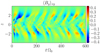 |
Fig. 1. (z, t)-diagram of the horizontally averaged toroidal magnetic field component ⟨By⟩xy for simulation 20pHbeta100. A butterfly pattern emerges shortly after the start of the simulation. |
We also tested whether the magneto-rotational instability is resolved in the chosen configurations. An approximate criterion for this is given by the ratio of the most unstable MRI wavelength (∼2πvA, i/Ω0, see e.g., Balbus & Hawley 1998) to the discretisation length of the grid (δxi = Li/Ni). The index i refers to the ith Cartesian component. The resulting quality factor is often referred to as QMRI (see e.g., Noble et al. 2010; Simon et al. 2011):
Hence, QMRI, i > 1 is required for the MRI to be resolved. Sano et al. (2004) found QMRI, z ≳ 6 as a criterion for MRI to be fully resolved. Time-averaged values ⟨QMRI, i⟩t are shown for all three configurations in Table 1. In all cases, one finds ⟨QMRI, y⟩t > ⟨QMRI, x⟩t > ⟨QMRI, z⟩t. The lowest value is ⟨QMRI, z⟩t = 7.4, observed for 20pHbeta100 and above the threshold found by Sano et al. (2004). Furthermore, as a clearly visible butterfly diagram emerges, the simulations are considered sufficiently resolved.
In MRI calculations, the turbulent stress has two contributions, the Maxwell part and the Reynolds part, see Eqs. (8) and (9). Time-averaged values of the stress contributions αr (Reynolds), αm (Maxwell), and α = αr + αm are listed in Table 1. For incompressible and isothermal MRI simulations, the factor (2/(3γ)) in Eq. (8) is often not considered. Hence, for better comparison with other MRI-related literature, that additional factor is not used for the values listed in Table 1. Also, the stresses are sometimes normalised by the mid-plane pressure instead of the volume-averaged pressure. Hence, values normalised by the mid-plane pressure at the start of the simulation P0(t = 0) are additionally provided in Table 1, designated  . The obtained values agree well with previous studies. Stone et al. (1996) found (αm = 0.0044, αr = 0.00125) for run ‘IZ1’ (compared to values
  in Table 1) and Simon et al. (2011) found (αm = 0.022, αr = 0.0058) for run ‘32Num’ (compared to values αm, r in Table 1).
In all three configurations, one finds Maxwell-to-Reynolds stress ratios in the αm/αr ≈ 3.6−3.8 (Table 1) range. This is typical for magneto-rotational turbulence and is often observed in simulations (see e.g., Hawley et al. 1995; Blackman et al. 2008; Simon et al. 2011; Riols & Latter 2018a).
Another quantity that is found to yield typical values for MRI turbulence is the ratio of Maxwell stress to magnetic pressure: rsp = ⟨⟨−BxBy⟩/⟨B2/2⟩⟩t (Hawley et al. 1995; Blackman et al. 2008; Simon et al. 2011; Hawley et al. 2011). Observed values often lie in the 0.3−0.4 range. For all three cases studied here, one finds a value of rsp ∼ 0.35 (see Table 1), which agrees well with the expected range for MRI. As we show below, this also holds for the GI-MRI combined state.
4.2. GI turbulence
In order to study purely gravito-turbulent states in stratified shearing box systems, Eqs. (2a)–(2f) are solved with B = J = 0. The cooling (heating) model used is that in Eq. (5), with the first term representing radiative cooling with cooling time τc and the second term accounting for irradiation heating with irradiation temperature ∝cs, 0. It is noted that in code units, cs, 0 = 1 (see Sect. 2).
We discuss four different configurations, which are shown as columns in Table 2. The four configurations differ in the total mass contained in the box volume. A convenient dimensionless measure for the mass content is the background Toomre value Q0, Table 2. Background here means that the constant value cs, 0 (irradiation) is used in Q0 instead of cs, and, hence, Q0 only depends on the volume-averaged mass density ⟨ρ⟩ (see also Sect. 2). The vertical boundary conditions allow mass to leave the box, causing Q0 to slightly evolve over time. As the latter effect is small, a time average ⟨Q0⟩t over an interval of  is provided in Table 2. Listed separately from the background value is the saturated Toomre value ⟨⟨Q⟩⟩t. The inner average ⟨Q⟩ is over the volume and calculated according to Eq. (7). The obtained values are then averaged over the respective time interval (outer brackets). It is noted that, in contrast to Q0, ⟨Q⟩ also depends on the saturated sound speed ⟨cs⟩ and is therefore also sensitive to the saturation level of the thermal energy density.
Hydrodynamical benchmark simulations with self-gravity.
The box dimensions are the same for all four simulations and are listed in the first three rows of Table 2. Box dimensions of 20H in both horizontal directions turned out to be reasonable for GI, avoiding bursting behaviour due to unstable modes fitting the box size as well as being reasonable in terms of computational effort. The horizontal box size is also similar to that used in Riols & Latter (2018a). The corresponding number of grid points is a compromise between computational accessibility and resolution, whereby the z resolution is chosen to be similar to the horizontal. Hence, the resolution is also comparable to (slightly higher than) that used for 20pHbeta100. Similar to the MRI cases, one has to take into account that the total number of processors used to parallelise over (x, y) is ideally divisible by 20. Hence, 440 points in both horizontal directions is a convenient choice (see also Appendix C). The chosen CFL number in all cases is 0.06. All simulations listed in Table 2 are restarted from an initial simulation that has been brought into the nonlinear state. At the restart time, the mass densities have been rescaled to yield different total box masses (⇒ different Q0; see Appendix B).
Mass-density snapshots for simulation GI072 are visualised in Fig. 2, with the first image showing a horizontal slice (x, y) and the second image depicting a vertical slice (x, z). In the bottom image, the base-ten logarithm of the mass density is used in order to provide a more convenient visual representation. In the (x, y) slice, one can see density waves and also shocks, separating the waves from lower density regions. Similarly to the findings in Riols & Latter (2018b), vortical motions above and below density waves are also observed. This is captured well in Fig. 3, which depicts an (x, z) slice of the mass density and the vertical stream lines for a fixed time point in the turbulent state of GI058. One can clearly observe four eddies symmetrically oriented around the density maximum near the centre of the image. The stream lines are traced only in the (x, z) plane, that is, neglecting the velocity component vy. The line colouring is such that motion away from the mid-plane is positive and motion towards the mid-plane is negative (sign(z) vz).
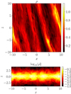 |
Fig. 2. Mass-density slices for GI072 in fully developed turbulence, |

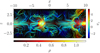 |
Fig. 3. Poloidal mass-density slice ρ(x, y = 0, z) with stream lines traced in the (x, z) plane. Stream-line colours are mapping the vertical velocity component away from the mid-plane (sign(z) vz). The stream lines are traced for one fixed point in time (t = const.) and by considering only the velocity components (vx, vz). |
In hydrodynamic, self-gravitating cases, the turbulent stress has two contributions: a Reynolds-part and a gravitational-part (see Eqs. (8)–(9)). Time averages of the dimensionless stress contributions αr (Reynolds), αg (gravitational), and α = αr + αg are provided in Table 2. The obtained values for α and αg are shown as a function of the saturated Toomre parameter ⟨⟨Q⟩⟩t in Fig. 4, whereby red dots correspond to αg and black stars correspond to α. The time averages for both α… and ⟨Q⟩ were taken over an interval of  in the fully developed turbulent state of each simulation. The MHD simulations sg-mhd-1 and sg-mhd-2 that will be discussed in later sections are shown as diamonds and crosses. The red dashed line is a guide for the eye (linear fit) for the trend in αg.
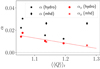 |
Fig. 4. Time-averaged dimensionless turbulent stresses (Eqs. (8) and (9)) as function of the volume and time-averaged Toomre parameter ⟨⟨Q⟩⟩t. Each data point corresponds to one simulation. The black stars show the sum total of Reynolds and gravitational stress α = αr + αg for the hydrodynamical simulations (GI058, GI072, GI087, GI095). The corresponding contributions from the gravitational stress αg are hown as red dots. Depicted as black diamonds and red crosses are α and αg for the MHD simulations sg-mhd-1 and sg-mhd-2 (discussed in the following sections). In MHD cases, one has α = αr + αg + αm, with Maxwell contribution αm. The red dashed line is a guide to the eye (linear fit) for the trend in αg. |
The energy balance is also tested in the nonlinear state. The only way the system can lose or gain energy is by extracting kinetic energy from the background shear flow (Kepler) or by radiative cooling and irradiation heating (Eq. (5)). Minor losses over the vertical boundaries may also occur. In a stationary state, the kinetic energy extracted from the Kepler shear (related to α) is balanced by net cooling and irradiation (related to  ). The balance can be used to derive a relation between the cooling rate and the dimensionless turbulent stress α (see Gammie 2001; Rice et al. 2011). For the cooling-model used here, this is
with P = (γ − 1)Eth. The values αp calculated via Eq. (17) are also shown in Table 2. As can be seen, for all simulations the αp are in good agreement with the values α obtained via Eq. (8), proving that the energy balance between turbulent dissipation and cooling is statistically satisfied with a high level of accuracy.
5. MHD simulations including self-gravity and irradiation heating
5.1. Initial conditions
To investigate interactions of the gravito-turbulent state with magnetic fields, a simulation with fully developed gravito-turbulence but no magnetic field is restarted introducing a magnetic seed field (see also the method used in Riols & Latter 2018a, 2019). The initial field is seeded into the turbulent state of GI072,  after the start of the simulation. This corresponds to the density slices shown in Fig. 2. It is noted that, unless stated otherwise, the time axes in all subsequent plots start at tΩ0 = 120, which is due to the fact that GI072 is restarted from an initial simulation (see Appendix B) and tΩ0 = 120 corresponds to the absolute time point when the seed field is introduced.
For simplicity, the aforementioned combined simulation is referred to as sg-mhd-1 in the following. The magnetic seed field is chosen such that β ∼ 1010, to make sure that no artefacts from the initial conditions arise. The initial seed-field configuration is of zero-net-flux type, with the field pointing in the z direction:


All hydrodynamic simulation parameters of GI072 are passed on to sg-mhd-1. This includes the radiative cooling model of Eq. (5), with a cooling-time of τcΩ0 = 10.
5.2. Observed time evolution
This section is used to report on some prominent features that are observed in the self-gravitating MHD simulations. More detailed discussions of some of the aspects are provided in subsequent sections.
The time evolution of the box-averaged magnetic energy density for sg-mhd-1 can be seen in the first image of Fig. 5 as the dashed and dotted lines, corresponding to the left abscissa. Most of the energy is in the y component ( , dotted line), followed by minor contributions from the x component (
 , dashed line) and the z component (
 , dash-dotted line). The system enters a growth phase immediately after initialisation, with the magnetic energy density increasing between five and eight orders of magnitude within 120 ≲ tΩ0 ≲ 400. The growth then stagnates for tΩ0 ≳ 400. In the latter phase, the volume-averaged magnetic field components are oscillating (see e.g., ⟨By⟩ as the black solid line in the first image of Fig. 5). The simulation sg-mhd-2 (red solid line) is discussed in more detail in the last paragraph of this section. ⟨By⟩ yields significantly larger oscillation amplitudes than the other components, and, during maxima, ∼30% of the total magnetic energy is assigned to ⟨By⟩2/2.
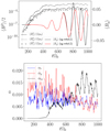 |
Fig. 5. Time evolution for a selection of volume-averaged quantities, whereby the first image shows quantities related to the magnetic field and the second image depicts the turbulent stresses. First image: left axis, dashed and dotted lines: box-averaged magnetic energy densities for Bx, By, and Bz. Right axis, solid lines: box-averaged toroidal field component ⟨By⟩ for simulations sg-mhd-1(black) and sg-mhd-2(red). Simulation sg-mhd-2 is discussed in the last paragraph of this section. Second image: turbulent stresses normalised by pressure sorted for αr (Reynolds), αg (gravity), and αm (Maxwell). The stresses (αr, αg) are smoothed using a Gaussian convolute (standard deviation |

In order to asses whether MRI can be active, one can calculate the QMRI, j parameters (Eq. (16)) for each field component, Bj, using the time evolution of the magnetic energy densities. First considered is the initial phase, 120 ≤ tΩ0 ≲ 400. Similarly to the energy densities, the QMRI, j also increase with time, and it is found that QMRI, y ≥ QMRI, x ≥ QMRI, z. Time averages over three different intervals in the initial phase are shown in Table 3.
As can be seen, QMRI, z < 1, except for the last interval. The z contribution is important as the Alfven component vA, z is connected to the most unstable MRI mode (see e.g., Sano et al. 2004). It was pointed out in Sano et al. (2004) that QMRI, z < 6 can lead to the decay of turbulence or significantly lower saturation levels (see also Sect. 1). In Simon et al. (2011), stratified, resistive, and viscous simulations are studied, and it is found that certain parameter regimes lead to time intervals of low turbulent activity. It is also mentioned that those intervals coincide with periods of unresolved poloidal magnetic fields, and turbulence sets back in once the shear has generated enough toroidal field strength By to restart turbulence. Hence, one concludes that MRI is, at maximum, marginally resolved in the early phases of sg-mhd-1. Especially in the interval 120 ≤ tΩ0 ≤ 200, all QMRI, j are significantly lower than one, and MRI is almost certainly absent. Further hints for this are also given in Sect. 6. Nevertheless, significant field amplifications are observed in that time period, as can be seen from the energy densities in Fig. 5. However, in the last image of Fig. 6 it is also observed that the ratio
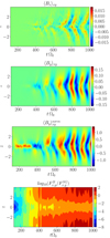 |
Fig. 6. (z, t) diagrams for different horizontally averaged quantities in sg-mhd-1. The first two images show the magnetic field components ⟨Bx⟩xy and ⟨By⟩xy, respectively. The third image shows |
relating horizontal forces due to the field line being bent to horizontal forces due to self-gravity, is significantly lower than one for tΩ0 ≲ 400. Here, the values shown in Fig. 6 are horizontal averages. It is noted that the field-line bending forces are also an important part of MRI. Weak magnetic pressure forces are guaranteed by the high initial thermal-to-magnetic pressure ratio β ∼ 1010. Hence, one concludes that MRI is most likely absent from the initial phase, and Lorentz forces in general are negligible compared to self-gravity forces. Consequently, one has to assume that the system would be stable without GI and the initial field amplifications must then be caused by kinematic effects of GI turbulence. This suggests that GI provides a possible dynamo mechanism. Additionally, in contrast to the low initial QMRI, j values, the saturation level of the QMRI, j is roughly two-to-three times larger than for the pure MRI simulations. For the toroidal component, this yields QMRI, y ∼ 50−90 for tΩ0 ≳ 600.
The second image in Fig. 5 shows the turbulent stresses normalised by the volume-averaged pressure, following Eqs. 8 and 9. It is noted that both αr and αm significantly fluctuate with time and are therefore smoothed by folding the time series with a Gaussian distribution (standard deviation  ).
).
Similarly to the magnetic energy, the Maxwell contribution to the stress (αm) is also increasing significantly and even becomes the dominant stress contribution for tΩ0 ≳ 700. This is in contrast to Riols & Latter (2018a), in which αg is the dominant contribution.
The volume-averaged toroidal field component ⟨By⟩ for sg-mhd-1 is shown in the first image of Fig. 5 as the solid black curve. For tΩ0 ≳ 400, clear oscillations with growing amplitude can be observed. We only show the y component, though the same oscillation occurs for the ⟨Bx⟩ component as well. This can also be seen in the horizontally averaged field components ⟨Bx⟩xy and ⟨By⟩xy, which are shown in the first two images of Fig. 6. The oscillations appear as a clearly regular pattern that closely resembles that of a butterfly diagram, similar to MRI turbulence (see e.g., Gressel 2010; Davis et al. 2010; Simon et al. 2011). Field reversals are also found in Riols & Latter (2018a), although they are much less regular and more concentrated to the mid-plane, especially for cooling times tΩ0 ≲ 20. The pattern obtained here appears to be more akin to that found in the global simulations of Deng et al. (2020).
The first of the bottom two images in Fig. 6 shows ⟨By⟩xy, except that the averaged field components are normalised by the root-mean-squared field, which is averaged over the entire box volume at that particular time point:  . From that, one can see that the initial phase tΩ0 ≲ 400 is qualitatively different from later times. One field reversal near the mid-plane is observed shortly before tΩ0 = 400, though this may already be a first manifestation of the emerging butterfly diagram. Also, the magnetic activity seems to be concentrated closer to the mid-plane, which is clearly in contrast to the butterfly-diagram that develops later. This initial state appears to be qualitatively closer to the state observed in Riols & Latter (2018a), where most of the activity is near the mid-plane and field reversals occur less regularly.
The last image in Fig. 6 shows the ratio of horizontal field-line bending forces,  , to horizontal self-gravity forces,
  , whereby the base-ten logarithm of the values is depicted. For tΩ0 ≲ 400, self-gravity clearly dominates (see also the discussion above), whereas for later times, forces due to field-line bending can significantly exceed self-gravity above and below the mid-plane (see also Sect. 6).
The total mass in the simulation volume (M = ⟨ρ⟩ Lx Ly Lz) starts to decrease once the magnetic field becomes more dominant tΩ0 ≳ 400. This trend is shown for the volume-averaged mass density ⟨ρ⟩ by the blue declining curve in Fig. 7. We interpret this as an increased wind activity at the vertical box boundaries. Something similar is also observed for the global simulations in Deng et al. (2020). One can take advantage of this by restarting sg-mhd-1 at a given time point (here tΩ0 = 600) and holding the total mass in the box volume constant from then on. This restarted simulation is referred to as sg-mhd-2 in the following. Consequently, sg-mhd-1 and sg-mhd-2 can really only be compared for tΩ0 > 600. Simulation sg-mhd-1 for tΩ0 > 600 and simulation sg-mhd-2 are exactly equal, with the only difference being that the total mass contained in the box volume is held constant in sg-mhd-2. Hence, the volume-averaged mass density ⟨ρ⟩ stays constant in sg-mhd-2, whereas it slowly decreases in sg-mhd-1 (see the dashed blue lines in Fig. 7). Clearly, at tΩ0 = 600 the values for ⟨ρ⟩ are exactly equal in sg-mhd-1 and sg-mhd-2. This reflects on the Toomre values ⟨⟨Q⟩⟩t and the latter split at tΩ0 = 600 with ⟨Q⟩ increasing for sg-mhd-1 and ⟨Q⟩ staying roughly constant for sg-mhd-2 (see the solid black lines in Fig. 7). This allows one to study the dependence of various quantities on the Toomre parameter in the presence of magnetic fields. For example, one now has two data points for MHD cases in Fig. 4 instead of only one. The last point is elaborated on in more detail in the next section. The replenishing is achieved by calculating the total box mass at each moment and comparing it to the original value (here at tΩ0 = 600). Once the mass deviates by more than 1%, the latter is restored to its original value by adding a density correction δρ at each grid point, such that the integral yields exactly the missing mass, ∫δρ dV = △M. Thereby, the density correction is distributed homogeneously over (x, y) and has a Gaussian profile in the z direction. Here,  with h = 0.5 is chosen. Between sg-mhd-1 and sg-mhd-2, no qualitative changes are observed, with the butterfly diagram, for instance, being unchanged. The box-averaged toroidal field component ⟨By⟩ for sg-mhd-2 is shown as the red, solid curve in Fig. 5, and it can be seen that no qualitative changes occur, except slight changes in frequency and amplitude. However, quantitative changes in the time-averaged stresses can be observed between sg-mhd-1 and sg-mhd-2. This is discussed in more detail in the next section.
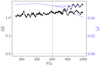 |
Fig. 7. Saturated Toomre parameter ⟨Q⟩ (solid black, left axis) and box-averaged mass density ⟨ρ⟩ (dashed blue, right axis). At tΩ0 = 600, sg-mhd-1 was restarted, with ⟨ρ⟩ held constant from then on (sg-mhd-2). Therefore, the values of ⟨ρ⟩ start to deviate between sg-mhd-1 and sg-mhd-2 at tΩ0 = 600. Similarly, the values of ⟨Q⟩ also begin to deviate at tΩ0 = 600. For sg-mhd-1, ⟨Q⟩ slightly increases, and for sg-mhd-2, ⟨Q⟩ stays almost constant. |
6. GI-MRI coexistence
6.1. Testing the presence of MRI
Table 4 lists important quantities averaged over both volume and time for simulations sg-mhd-1 and sg-mhd-2. For sg-mhd-1, two different time intervals are considered for the average, 120 ≤ tΩ0 ≤ 320, left column, and 700 ≤ tΩ0 ≤ 1000, middle column. The first time interval corresponds to the previously discussed initial phase, where the most unstable MRI mode is significantly under-resolved and where MRI is therefore most likely absent. This is further backed up below. Listed in the third column are time averages for sg-mhd-2 (mass held constant) using the second time interval (700 ≤ tΩ0 ≤ 1000).
Selection of volume- and time-averaged quantities for simulations sg-mhd-1,2.
In sg-mhd-1, the time-averaged αm is dominant for 700 ≤ tΩ0 ≤ 1000, whereas αg has decreased by roughly 50% compared to the 120 ≤ tΩ0 ≤ 320 interval. The Reynolds contribution αr is also reduced by ∼20%, which is significantly less than the reduction of αg. The total stress (α = αr + αg + αm) increases from the first to the second time interval by ∼14%, which can be attributed to the emergence of αm for tΩ0 ≳ 400. Also shown in Table 4 is the predicted total stress, αp, calculated from the energy balance between turbulent production and radiative cooling (heating) (Eq. (17)). In the low stress interval (120 ≤ tΩ0 ≤ 320) of sg-mhd-1, both α and αp are in good agreement, indicating that most of the energy extracted from the background is eventually lost through radiative cooling. In the second interval (700 ≤ tΩ0 ≤ 1000) of sg-mhd-1, the αp-value did not change, but the total stress α increased by ∼14%. This agrees with the observed loss of mass, as the generation of a wind will also lead to an additional energy flux that is not accounted for by radiative cooling. Hence, the most dominant effect of introducing magnetic fields is that the gravitational stress αg is decreasing, whereas the Maxwell stress αm is increasing and also overcompensating the reductions of both αg and αr.
As it turns out, the reduction of αg in sg-mhd-1 from the first to the second time interval is related to an increase in the saturated Toomre parameter, ⟨Q⟩. The reason for changes in ⟨Q⟩ is twofold. The dominant reason in sg-mhd-1 is that, as discussed in Sect. 4, winds at the vertical boundaries lead to a sinking mass in the box volume, thereby increasing both the irradiation-Toomre Q0 as well as the saturated value ⟨Q⟩ (see Table 4). The second reason includes changes in the saturated thermal energy density. The irradiation value Q0 does only react to changes in mass as the irradiation temperature is held constant (cs, 0 = const.), but the saturated value ⟨Q⟩ can change due to thermal energy changes as it also depends on the saturated sound-speed ⟨cs⟩. Hence, the ⟨⟨Q⟩⟩t-difference between sg-mhd-2 and sg-mhd-1 is in part due to the higher mass in sg-mhd-2 (mass held constant), but also due to the slightly different saturation levels of the thermal energy density (see Table 4).
Regardless of the exact changing mechanism, the difference of ⟨⟨Q⟩⟩t between sg-mhd-1 and sg-mhd-2 allows one to investigate the dependence of αg on the saturated Toomre-parameter ⟨⟨Q⟩⟩t for the MHD cases. It turns out that the reduction of the time-averaged αg from the first to the second time interval is only 33% for sg-mhd-2 compared to 50% for sg-mhd-1 (see Table 4). A possible trend can be directly analysed using Fig. 4. The dimensionless gravitational stresses αg are shown for sg-mhd-1,2 (700 ≤ tΩ0 ≤ 1000) via the two red crosses in Fig. 4, whereby the lower αg value corresponds to sg-mhd-1 (see also Table 4). These values can then be compared to αg, obtained from the purely hydrodynamical GI-simulations and shown as red dots. One can clearly see a trend for αg as a function of ⟨⟨Q⟩⟩t. The data point obtained for sg-mhd-2 is especially close to a hydrodynamical simulation (GI087). It is stressed at this point that sg-mhd-1 (and therefore sg-mhd-2) is restarted initially from GI072 by introducing a seed field. Hence, it appears that the newly formed turbulent states with magnetic fields lead to significantly different values in both ⟨⟨Q⟩⟩t and αg; though, the dependence αg(⟨⟨Q⟩⟩t) remains similar to the hydrodynamical states. This is clearly not the case for the total stress α = αr + αg + αm. From Fig. 4, one can see that simulations sg-mhd-1,2 (black diamonds) deviate significantly from the trend observed for the purely hydrodynamical cases (black stars). This is of course attributed to the emergence of a strong magnetic stress contribution αm (see also Table 4). Despite αg being larger for sg-mhd-2 compared with sg-mhd-1, one can see from Table 4 that the total stress (α = αr + αg + αm) for sg-mhd-2 is exactly equal to that found for sg-mhd-1. Consequently, αm is found to be lower in sg-mhd-2 compared to sg-mhd-1. What this suggests is that GI with magnetic fields is qualitatively similar to purely hydrodynamic GI; though, the presence of magnetic fields may have an influence on the Toomre-parameter and thereby on the absolute strength of GI, as measured in αg.
It then remains to be tested whether the magnetic stress-contribution αm originates from MRI-turbulence. As shown by the previous considerations, the introduction of magnetic fields did not change the turbulence characteristics of GI, although the absolute values ⟨⟨Q⟩⟩t and αg can change. Therefore, a simple superposition may be assumed and the turbulent stress is separated into two contributions: α = α(GI)+α(MRI). The magnetic part αm then originates from MRI and the gravitational stress αg originates from GI. The Reynolds part has contributions from both MRI and GI. Hence, the following separation of α is suggested:
Therein, the Reynolds stress has the contributions αr = αr(GI)+αr(MRI). One then determines the relations of (αm with αr) and (αg with αr) for pure MRI and pure-GI states, respectively. More precisely, the ratios Fm = αm/αr for MRI and Fg = αg/αr for GI are defined. It is noted that this assumes the ratios Fg and Fm to be set independently from each other. Hence, the presence of MRI does not affect Fg and GI does not affect Fm. It is again noted that this is supported by the previous considerations, showing that the hydrodynamical trend for αg can be extended to the MHD cases as well. To see whether the combined states, sg-mhd-1 and 2, are consistent with the independently set values of Fm and Fg, one first determines the ratio Fg from GI simulations and then calculates the resulting Fm. Simulations of magneto-rotational instability suggest typical values of 3.6 ≲ Fm ≲ 4.0 (see Sect. 4.1 and Sect. 8 below). Values for Fg are obtained from the pure GI simulations discussed in Sect. 4 and are listed in the last row of Table 2. One could have started with Fm and derived Fg from that, but Fm is rather a fixed (typical) value, whereas Fg can depend on the mass content measured by Q0, as can be seen in Table 2. As Table 2 provides Fg for simulations with different total box masses and therefore different values of ⟨Q0⟩t, one can estimate the Fg for sg-mhd-1 (reduced mass) and sg-mhd-2 (constant mass) by interpolating between the values in Table 2. For sg-mhd-1 one thereby finds ⟨Q0⟩t = 0.86 leading to Fg ≈ 2.0 and for sg-mhd-2 it is ⟨Q0⟩t = 0.75 leading to Fg ≈ 1.85.
In the combined state, one has Fg = αg/(αr(GI)) and as αr = αr(MRI)+αr(GI), one finds αr(MRI)=αr − αg/Fg. This is then substituted in Fm = αm/(αr(MRI)), yielding
Applying Eq. (22) to the values for sg-mhd-1 and sg-mhd-2 (second and third column in Table 4), one finds
Hence, the values are in very good agreement with the expectation for MRI turbulence. This also demonstrates that the combined state is consistent with a coexistence of GI and MRI, whereby the ratios Fg and Fm are set independently from each other. For comparison, one can also evaluate Fm for the initial phase 120 ≤ tΩ0 ≤ 320 of simulation sg-mhd-1 (first column in Table 4). There, one finds ⟨Q0⟩t ∼ 0.72, which is expected, as sg-mhd-1 is restarted from GI072 and the initial magnetic fields are weak. From Table 2 then follows Fg = 1.8. Using the time averages in Table 4 and applying Eq. (22), one obtains Fm = 0.223 ≪ 4. This is further proof supporting the argument in Sect. 5.2 that MRI is absent from the initial phase of sg-mhd-1. It also shows that, even when GI is corrected for, the kinematic stress contributions dominate the magnetic contribution and the fields are likely passive in the initial phase. This further strengthens the picture that the initial field amplification is caused by GI turbulence. This is of course significantly different from the saturated state primarily studied in this section.
Similarly to the pure MRI simulations, one can also check for the ratio of Maxwell stress to magnetic pressure rsp = ⟨⟨−BxBy⟩/⟨B2/2⟩⟩t. For sg-mhd-1, we find rsp = 0.32, and for sg-mhd-2 rsp = 0.34, whereby the time averages are evaluated for 700 ≤ tΩ0 ≤ 1000. Hence, the ratio also agrees well with the ratios obtained for the pure MRI simulations (see Sect. 4.1).
The coexistence hypothesis is further backed up by the last image in Fig. 6, depicting the ratio of horizontal field-line bending forces to horizontal forces of self-gravity  , evaluated for sg-mhd-1. As can be observed in Fig. 6, values of
  occur for tΩ0 ≳ 400. The ratio increases with |z|, and for higher altitudes one even finds values up to ∼100 and the bending forces clearly dominate. Only near the mid-plane (|z|≲1H) does one find self-gravity forces to be significantly larger than field-line bending. Since the instability mechanism of MRI relies on field-line bending forces (see e.g., Balbus & Hawley 1998), this is a strong indication that the latter is active, at least for higher altitudes.
6.2. Discussion and comparison to previous studies
At this point, it is useful to present a short discussion about the interpretation of the previously obtained results and also to give a comparison to the findings for the non-irradiated cases studied in Riols & Latter (2018a). First, an overview of similarities and differences to the setup of the SGMRI simulations in Riols & Latter (2018a) is given. The similarities are discussed first. One of them is the horizontal box size, which is 20H in both the x and the y direction. The horizontal resolutions are also similar, whereby Riols & Latter (2018a) used ∼26 points per H, and here, 22 points per H are used. This is true for the vertical resolution as well, which is ∼21 point per H in both cases. The boundary conditions are also similar for both setups. These are outflow-type boundaries for the velocity and vertical-field boundary conditions for the magnetic field. An important difference is the cooling model. In addition to a pure cooling function, the model used here also includes a heating term (see the second term in Eq. (5)). The latter is not used in Riols & Latter (2018a). Additionally, the vertical box size used here (−4H < z < 4H) is slightly larger than the size used in Riols & Latter (2018a) (−3H < z < 3H). The comparison provided here especially refers to the SGMRI-(...) simulations in Riols & Latter (2018a), as they also introduced a magnetic seed field into a gravito-turbulent state. It is noted that Riols & Latter (2018a) also provided simulations starting with an MRI state and introducing self-gravity, whereby no significant differences are observed.
Now, differences in the simulation outcomes are elucidated. One difference is the saturation level of the turbulent stresses. Here, it is found that αm is the dominant contribution in both simulations sg-mhd-1 and 2 and the stresses αg and αr are of the same order of magnitude. This is in contrast to SGMRI-10 (τcΩ0 = 10) in Riols & Latter (2018a). There, αm and αr are of the same order of magnitude and αg is the dominant contribution. Moreover, the relative strength of αm is even weaker for higher cooling times. Differences are also observed in both the time evolution and the vertical structure of the magnetic field. Our simulations sg-mhg-1 and 2 both develop butterfly diagrams with clearly distinguishable field oscillations (see Fig. 6). Furthermore, magnetic activity extends to higher altitudes. This is a distinguishing feature of Riols & Latter (2018a), in which more irregular field reversals were found, and for cooling times τcΩ0 < 100 the magnetic activity is mainly confined to the mid-plane region. It is noted that the concentration of magnetic activity near the mid-plane is also found here, though this is only in the early phases tΩ0 ≲ 400 where MRI is not resolved or fully developed. We agree with Riols & Latter (2018a) that GI provides a dynamo (see the initial field amplification between  and
and  ). However, it is found that this does not imply suppression of MRI for efficient cooling (τcΩ0 = 10), but rather that the saturated state is characterised by a coexistence of both.
It is noted at this point that the previously discussed simulations do include the effect of irradiation heating (second term in Eq. (5)), which is not the case in Riols & Latter (2018a). Whether the differences are due to the influence of irradiation is elucidated in Sect. 7 below. The boundary conditions used here are comparable to those used in Riols & Latter (2018a); hence, the differences are unlikely to arise from boundary artefacts.
From the previously derived results, one concludes that the turbulent states of simulations sg-mhd-1 and 2 consist of a coexistence between MRI and GI. However, this does not mean that the stresses can simply be added, as is also pointed out in Riols & Latter (2018a). Equation (26) may seem to do that, but it is noted that the saturation value of the Toomre-parameter ⟨Q⟩ also changes with the introduction of magnetic fields. Hence, this is different than adding MRI stresses to the GI stress before magnetic fields have been introduced, as the presence of magnetic fields has an influence on the overall energy balance. Here, the changes in ⟨Q⟩ are in part due to mass changes, but even with constant mass, the additional Maxwell stress −BxBy provides additional means to extract energy from the background flow and thereby to change the saturation level of thermal energy.
Finally, it is noted that the results obtained here are more akin to the findings in the global simulations of Deng et al. (2020). There, hints for field-oscillations reminiscent of a butterfly diagram are found as well. Furthermore, the ‘grvmhd1’ simulation in Deng et al. (2020) develops a Maxwell stress in excess of the other stress contributions, which is also a common feature of the simulations presented here.
7. The influence of irradiation-heating
All previous simulations include irradiation heating (second term in Eq. (10)), which is not the case for the simulations in Riols & Latter (2018a). As notable differences arise in the previous chapters, the influence of irradiation will be elucidated in more detail here. For that purpose, restarts are conducted from sg-mhd-1 at tΩ0 = 920. For the restarts, irradiation is turned off and the total mass held constant. Two different restarts are run, with the first changing the cooling time to τcΩ0 = 20 (sg-mhd-noirrad-20) (a more detailed discussion is provided for that cooling time in Riols & Latter 2018a) and the second keeping the original cooling time τcΩ0 = 10 (sg-mhd-noirrad-10).
The restart of sg-mhd-noirrad-20 is done in two steps. At tΩ0 = 920, irradiation is turned off, and later, at tΩ0 = 1060, the cooling time is set to τcΩ0 = 20.
The horizontally averaged toroidal field component ⟨By⟩xy is depicted for sg-mhd-noirrad-20 as functions of z and t in the first image of Fig. 8. As can be seen, the butterfly diagram is at first disrupted but eventually returns. The resulting state is qualitatively different from that found for SGMRI-20 in Riols & Latter (2018a). It is noted that for sg-mhd-noirrad-10, the field oscillations become more irregular near the mid-plane (|z|≲1H), but the butterfly is still visible for higher altitudes. The second image of Fig. 8 depicts the dimensionless turbulent stresses αr, αg, and αm as a function of time. Averaging the stresses over time, starting at tΩ0 = 1100 yields the values listed in the first line of Table 5. The corresponding values found in Riols & Latter (2018a) (SGMRI-20) are shown in the second line. The same is also shown for sg-mhd-noirrad-10 (third line) and the respective SGMRI-10 simulation of Riols & Latter (2018a) (fourth line).
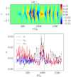 |
Fig. 8. Time evolutions of the vertical magnetic field structure and the dimensionless turbulent stresses for simulation sg-mhd-noirrad-20. First image: horizontally averaged field component ⟨By⟩xy as function of (z, t). Second image: dimensionless turbulent stresses (αr, αg, αm). Stresses (αr, αg) were smoothed using a Gaussian convolute (standard deviation |

Time-averaged, dimensionless, turbulent stresses for cases without irradiation: sg-mhd-noirrad-10 (τcΩ0 = 10, first line) and sg-mhd-noirrad-20, (τcΩ0 = 20, second line).
The stresses for SGMRI-20 and SGMRI-10 were obtained by applying Eqs. (8) and (9) to the values provided in Riols & Latter (2018a) (see also Appendix D). In addition to the stresses, the ratio of Maxwell stress to magnetic pressure rsp = ⟨⟨−BxBy⟩/⟨B2/2⟩⟩t is provided in the last column.
As one can see, all stress contributions (αr, αg and αm) in sg-mhd-noirrad-10 are comparable to those obtained in SGMRI-10. Regarding the ratio rsp, both simulations yield values from 0.3−0.4, which is also typical of MRI. The situation is different for sg-mhd-noirrad-20 and SGMRI-20, with the stresses differing significantly. The Reynolds-contribution αr is mostly similar in both cases, but the Maxwell and gravitational contributions switch places. In sg-mhd-noirrad-20, the Maxwell part αm is dominant whereas in SGMRI-20 the gravitational contribution αg is dominant. Also, the magnetic stress-to-pressure ratio for sg-mhd-noirrad-20 is rsp ∼ 0.32, which is also MRI typical, but for SGMRI-20 it is found to be rsp ∼ 0.28, which is considerably lower than all other values. We also analysed the sum total stress α for both cooling times. One first notices that the cases of Riols & Latter (2018a) and our simulations agree in that their α values differ by roughly a factor of two between τcΩ0 = 10 and τcΩ0 = 20. This finding is reasonable, considering that the total stress α is a measure of the rate at which energy is drawn from the Kepler flow and that the cooling timescale is a measure of how fast the system can lose thermal energy. Assuming a steady state, the extracted energy must be balanced by the losses. Reducing the τcΩ0 by a factor of two means doubling the energy-loss rate, which correlates with a doubling of turbulent energy production α. However, considering each cooling time separately, the α values found in Riols & Latter (2018a) and the values found here differ by ∼10%. One likely reason for the differences in α might be different rates of wind cooling. It may also be speculated that this is related to the other differences observed for τcΩ0 = 20 as well. This is also supported by the observed butterfly pattern, as the latter is characterised by magnetic activity rising to higher altitudes. Hence, this is likely an interesting route for future investigations.
One concludes that for τcΩ0 = 10 we can partly reproduce the results obtained in Riols & Latter (2018a), especially that the turbulent stresses are comparable. Although, for τcΩ0 = 20, significant differences arise. Although we currently have no clear explanation for the latter differences, one might speculate that they are related to wind activity at higher altitudes. Furthermore, we come to a different conclusion regarding the coexistence of GI and MRI. Similarly to the irradiated cases, the ratio of Maxwell stress to magnetic pressure is typical of MRI in both cases, and for τcΩ0 = 20 one finds a clearly visible butterfly pattern. Hence, a GI–MRI coexistent state can also be sustained without irradiation, and MRI is not suppressed.
8. Turning off self-gravity
To elaborate on the role of self-gravity, the simulation sg-mhd-1 is restarted at tΩ0 = 920, with the influence of self-gravity being effectively removed. For that purpose, the gravitational constant is rescaled by a factor of 100 (G = 1 → G = 0.01). That simulation is run until tΩ0 = 1520 and is referred to as sg-mhd-G001. Time evolutions of the ⟨By⟩-field component and the magnetic energy densities are shown in the first image of Fig. 9. The vertical dashed line marks the time point of rescaling, tΩ0 = 920. The energy densities are mapped to the left abscissa, with curves for  (black, dashed),
  /2 (blue, dotted), and
  (red, dash-dotted). The ⟨By⟩-component is mapped to the right abscissa as the black solid curve. Shown in the second image of Fig. 9 is the toroidal field component, averaged horizontally ⟨By⟩xy and as function of (z, t), whereby t starts at
  .
.
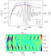 |
Fig. 9. Time evolution for a selection of volume-averaged quantities, related to the magnetic field, and the evolution of the vertical magnetic field structure, for simulation sg-mhd-G001. First image: volume-averaged magnetic energy densities separated into components |

Some observations can immediately be made. The volume-averaged magnetic energy densities decrease significantly. Comparing the time intervals (500 ≤ tΩ0 ≤ 920) and (1200 ≤ tΩ0 ≤ 1520), one finds that  decreases by 92%,
  by 84%, and
  by 93%. The oscillations in the volume-averaged ⟨By⟩ component also have significantly lower amplitudes and appear to be less regular without self-gravity. The oscillation frequency stays roughly equal. The butterfly diagram remains, although the mid-plane activity is significantly reduced (see the second image of Fig. 9).
As the magnetic field energy drops by roughly an order of magnitude, one concludes that the GI dynamo dominates in generating the magnetic field. One also concludes that the influence of GI is especially pronounced near the mid-plane, which is expected, as self-gravity has the most influence there. This also agrees with the last image in Fig. 6 (sg-mhd-1), indicating that Lorentz-forces can exceed self-gravity forces, especially for higher altitudes. The potential of GI to act as a dynamo is also consistent with the findings in Riols & Latter (2018a, 2019). The image that emerges is that MRI is operating on the field generated by the GI-dynamo, thereby leading to nonlinear saturation in the butterfly pattern. It is noted that the lack of coherence in the oscillations in the top image of Fig. 9 probably originates from a decoupling of the regions above and below the mid-plane, with the latter two regions in turn oscillating slightly out of phase. This then causes the volume-averaged values to oscillate more irregularly. The less regular oscillations are also present in the smaller box MRI simulations of Sect. 4.1.
Finally, the fact that one obtains a turbulent state for 1200 ≤ tΩ0 ≤ 1520 is further proof that in the original simulations one does have both GI and MRI. The stresses found in the new turbulent state are αm = 0.0024 and αr = 0.00058, yielding a ratio of αm/αr ≈ 4.1, which, as expected, agrees with the typical value for MRI.
9. Dynamo properties
Decomposing the velocity (v = (3Ω0/2)xey + δv) into background shear and perturbation δv, one can analytically show that the induction equation (Eq. (2d)) is of the following form:
with electromotive force ℰ = δv × B (see also Vishniac & Brandenburg 1997; Guan & Gammie 2011; Simon et al. 2011). A horizontal average is applied, yielding for the x and y components, respectively (see also Riols & Latter 2019),
It is then assumed that the connection between turbulent electromotive force and averaged field is of the form  , with coefficients
  and i, j ∈ {x, y}. The z derivatives in the induction equation are estimated to be of the order of ∂z ∼ 1/H. Substitution into Eqs. (25)-(26) and averaging over z yields (see also Guan & Gammie 2011)
It is noted that in the two equations above, the more convenient coefficients  ,
,  ,
,  and
and  are defined and are also used throughout the paper.
Depending on the exact choice of the αij, oscillations in ⟨Bx, y⟩ will occur. As Eqs. (27a)–(27b) are linear in the field components, one can analytically solve the model with an ansatz of the form ⟨Bj⟩=Ajexp(s t), whereby the both s and the Aj are complex numbers. Elementary analytical calculations then yield

The second term on the right hand side of Eq. (28a) is important for oscillations. For (Tr/2)2 − D < 0, the solutions oscillate with a frequency of  . In the simpler case of vanishing diagonal elements, αxx, αyy, the condition for oscillation reduces to αxy (αyx − 1.5Ω0)< 0. In case oscillations are present, the growth or decay of the latter is set by whether Tr/2 is positive or negative.
All simulations carried out in this study show field oscillations in the form of butterfly diagrams. In the early phases of sg-mhd-1 (tΩ0 < 400), sign reversals of both ⟨Bx⟩ and ⟨By⟩ occasionally occur. This is in contrast to Riols & Latter (2018a), in which irregularly occurring field reversals were found (more akin to the initial phase of sg-mhd-1), and also to Riols & Latter (2019), with field reversals being absent completely.
To test how the simulations relate to the simple dynamo-model of Eqs. (27a)–(27b), correlations between the time derivatives ∂t⟨Bi⟩ and the components themselves ⟨Bj⟩ were studied. This is visualised in the scatter plots of Fig. 10, with ∂t⟨Bi⟩ mapped to the y-axis and ⟨Bj⟩ mapped to the x-axis. Two subsequent time points in the scatter plots are separated by  , and the time derivatives are explicitly calculated from that. The set of all dots corresponds to the time interval (700 ≤ tΩ0 ≤ 1000) of sg-mhd-2. Shown in the legends are the slopes and y incidents, which were determined via linear regression. The appearance of ellipsoidal shapes in some plots is an indication that non-zero diagonal elements αxx and αyy also contribute. As H = 1 in code units, the slopes can be identified with the coefficients αij (see Eqs. (27a)–(27b)). The resulting coefficients are summarised in Table 6.
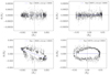 |
Fig. 10. Time derivatives of the volume-averaged magnetic field components ∂t⟨Bi⟩ as functions of the field components themselves ⟨Bj⟩. Each dot corresponds to a given time point in the interval (700 ≤ tΩ0 ≤ 1000) of sg-mhd-2, separated by |

A peculiarity arises for the coefficient αyx, as determining the latter also requires subtracting the shear (−1.5Ω0), that is, αyx = slope + 1.5. Directly reading off the slope from the bottom left image of Fig. 10, one finds the slope ≈ − 1.3. From this, one concludes that the effect of shearing (often called the Ω effect) is the dominant source for ⟨By⟩ production.
The αyx can be calculated more directly by evaluating the term ⟨∂z⟨ℰx⟩xy⟩z in Eq. (26) as function of ⟨Bx⟩, thereby avoiding to calculate the time derivative. Generating a similar scatter-plot with this term instead, yields αyx ≈ 0.197. That is in very good agreement with the value derived by explicitly calculating the time derivative ∂t⟨By⟩, providing a direct check.
The analytical dynamo model in Eqs. (28a)–(28c) is then applied to the values in Table 6, yielding

This implies that oscillations should be present in agreement with the observed butterfly diagram. From ω = 2π/T, one finds a time period  . The actual time evolution of ⟨By⟩, evaluated for sg-mhd-2, is shown via the red solid curve in Fig. 5. The dominant frequency obtained by calculating the Fourier series for the interval (700 ≤ tΩ0 ≤ 1000) yields a period of
  . Hence, the measured period is of the same order of magnitude as the period predicted by the model, though they are not exactly equal. The predicted growth rate (Tr/2) is found to be two orders of magnitude lower than the frequency part, which is considered an indication that the simulation is in a quasi-steady state, as amplitude growth stagnates. Doing the same analysis for (400 ≤ tΩ0 ≤ 700), one finds s ≈ 0.0022 ± i ⋅ 0.031. The frequency is roughly equal in both intervals, though the growth rate is one order of magnitude larger in the earlier time interval. This is expected, as the amplitude growth can clearly be observed for (400 ≤ tΩ0 ≤ 700) (see Fig. 5).
Riols & Latter (2019) proposed a possible mechanism for the GI-dynamo, which involves horizontal rolls (see Riols & Latter 2018b) above and below the density waves in the mid-plane. These rolls are indeed observed in the simulations presented in this paper (see Fig. 3). Also seen in Fig. 3 is that neighbouring rolls often rotate with opposite orientation. Furthermore, as the rolls are connected to density waves, the rolls are often not exactly parallel to the y-axis. Thus, a magnetic field with only a By component can be bent by neighbouring rolls to locally produce a Bx component (see the mechanism proposed in Riols & Latter 2019).
As the horizontal rolls appear slightly above and below the mid-plane (see Fig. 3), they tend to separate the upper atmosphere regions from the mid-plane. In order to demonstrate this, the horizontally averaged enstrophy  is calculated, whereby only the y vorticity ωy = ∂zvx − ∂xvz is considered. The enstrophy value is normalised by the mean-squared velocity perturbation ⟨δv2⟩xy in order to isolate changes in the vortical structure from changes in the magnitude of the velocity. The vertical profile,
  , obtained by averaging over the time interval (700 ≤ tΩ0 ≤ 1000), is depicted in Fig. 11, right abscissa. It is noted that the time average is obtained by evaluating
  for ten equidistant time points in the considered interval. As can be seen from Fig. 11, the enstrophy has pronounced maxima at |z|≈1H, separating the inner regions from regions in the upper atmosphere. Shown in black (left y-axis) are the two contributions to the electromotive force (ℰy = vzBx − vxBz), ⟨⟨vxBy⟩xy⟩t (dashed) and ⟨⟨vzBx⟩xy⟩t (dotted). The horizontally averaged magnetic field components periodically change sign, and so do the terms ⟨viBj⟩xy. For that reason, the ⟨viBj⟩xy are multiplied with the sign of the volume-averaged field component ⟨Bx⟩ at that particular time point. An average over the time interval (700 ≤ tΩ0 ≤ 1000) with ten equidistant time points then yields the black curves in Fig. 11. It can be seen that both ⟨⟨vxBz⟩xy⟩t and ⟨⟨vzBx⟩xy⟩t change behaviour at |z|≈1H, and on average ∂z(vxBz) and ∂z(vzBx) change sign at |z|≈1H. This is a strong hint that the rolls indeed play an important role in the dynamo mechanism (Riols & Latter 2019).
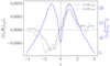 |
Fig. 11. Vertical profiles for a selection of quantities (averaged over (x, y), and over time). Left (vertical) axis: Vertical, turbulent shearing (⟨vxBz⟩xy, black dashed line), and vertical compression (⟨vzBx⟩xy, black dotted line) as a function of z. Right (vertical) axis: Toroidal enstrophy normalised by the mean-squared velocity perturbations ( |
This is further addressed in Table 7, which shows the αij one obtains if the field components are not averaged over the entire box height, but only over given height intervals. Two intervals are chosen, separating the mid-plane region |z|< 1H (interval I1) and the region above the mid-plane |z|> 1H (interval I2). This also coincides with the regions below and above the rolls, respectively. The values are calculated by reconstructing the ∂t⟨Bi⟩ from ∂z(⟨ℰj⟩xy) and averaging over the corresponding height interval in z. The frequencies can also be calculated for intervals I1 and I2, yielding s1 = 0.000251 ± i ⋅ 0.0505 and s2 = 0.00535 ± 0.0101, respectively. In terms of time periods, that is  for I1 and
  for I2. The mid-plane value is by far the closest to the observed butterfly frequency of
  , indicating that the frequency is predominantly set near the mid-plane.
αij coefficients for simulation sg-mhg-2 (700 ≤ tΩ0 ≤ 1000) and averaged over different altitudes.
The values in Table 7 demonstrate that the dynamo properties do change as a function of z. At higher altitudes, the Ω-effect is less dominant over the turbulent contributions compared to the volume near the mid-plane. αxy decreases towards higher altitudes. Though, the diagonal elements both increase significantly from the mid-plane to the higher regions. This is in agreement with the situation depicted in Fig. 11 suggesting that the dynamo changes properties at |z|≈1H.
The simulations presented here are hence consistent with the dynamo mechanism based on rolls, as proposed in Riols & Latter (2019); yet, we come to the opposite conclusion in terms of oscillations. In Riols & Latter (2019), the average field grows without sign reversals; although, it has to be noted that Riols & Latter (2019) also included a finite resistivity. The ideal runs in Riols & Latter (2018a) also show field reversals, though they are much less regular than the butterfly pattern found here. In our understanding, the model relying on the rolls connected with the density waves naturally predicts field reversals. Consider a purely toroidal magnetic field line with By > 0. The mechanism in Riols & Latter (2019) then suggests that the field line is lifted upwards between two neighbouring rolls. As the rolls are not perfectly aligned with the y-axis, some parts of the field line come to rest on the first roll, and other parts on the second roll. As the rolls rotate in opposite directions, the field line is bent between the two rolls, producing a positive Bx component. This is in agreement with the observation that αxy is positive. However, the thus produced Bx > 0 is subjected to shear, producing a δBy < 0. Hence, the newly produced y field has opposite sign to the original field. That will lead to the originally positive By being reduced and eventually crossing By = 0.
10. Summary
We first investigated the direct interaction of gravitational turbulence with magnetic fields by introducing a magnetic seed field into a gravito-turbulent state (simulation sg-mhd-1, with cooling time τcΩ0 = 10). Significant amplifications in the magnetic energy density and the volume-averaged fields can be observed in the initial phase, shortly after introducing a magnetic seed field. After  , the system changes state and a butterfly diagram develops that also extends towards higher altitudes in the z direction. This is in contrast to earlier studies of Riols & Latter (2018a) finding field reversals to occur much less regularly and magnetic activity to be more localised in the mid-plane region. It is noted that a concentration near the mid-plane is found in simulation sg-mhd-1 as well; though, this only occurs in the aforementioned initial phase after introducing the seed-field.
In accordance with the growing magnetic field strength, a Maxwell contribution αm to the total stress also emerges. As αm grows, the gravitational stress αg is found to decrease, whereas the sum total of all stresses slightly increases. At saturation, αm is the dominant stress contribution, or at least it is of the same order of magnitude as the remaining stress contributions. The reduction in αg is found to be consistent with an increase in the saturated Toomre parameter ⟨Q⟩. In simulation sg-mhd-1, this can mostly be attributed to a reduction of the total mass in the box volume due to vertical wind activity initiated by the magnetic fields. A second simulation (sg-mhd-2) is restarted from the early turbulent state of sg-mhd-1, whereby the sum total mass is then held constant. Hence, the mass is slightly higher in sg-mhd-2, leading to slightly lower ⟨Q⟩ values, and αg indeed saturates at a slightly higher level in sg-mhd-2 compared to sg-mhd-1. The total stress α is equal in both cases (sg-mhd-1 and 2), consequently, the saturation value αm is lower in sg-mhd-2 compared to sg-mhd-1. In addition to that, a method of separating possible GI and MRI stress contributions (α = α(GI)+α(MRI)) is suggested, and it is found that αm/αr(MRI)=3.85, 4.09 for sg-mhd-1 and 2, respectively. For the ratio of Maxwell stress to magnetic pressure, one obtains values of ⟨⟨−BxBy⟩/⟨B2/2⟩⟩t = 0.32, 0.34 for sg-mhd-1 and 2, respectively.
The influence of irradiation is demonstrated by using two restarts of sg-mhd-1, with irradiation being turned off at the restart point. One restart also changes the cooling time from τcΩ0 = 10 to τcΩ0 = 20. Both cases still develop butterfly diagrams, whereby the pattern is more pronounced for τcΩ0 = 20. For τcΩ0 = 20 especially, the clearly visible butterfly pattern is different from the findings for SGMRI-20 in Riols & Latter (2018a). The ratio of Maxwell stress to magnetic pressure ⟨⟨−BxBy⟩/⟨B2/2⟩⟩t is found to yield values similar to those obtained with irradiation. The averaged stresses for τcΩ0 = 10 are closest to the values found in Riols & Latter (2018a) (SGMRI-10), though for τcΩ0 = 20 significant differences remain. Most notably, the Maxwell contribution to the dimensionless stress αm is dominant for the cases presented here, whereas in (SGMRI-20) of Riols & Latter (2018a), the gravitational contribution is dominant αg.
The role of self-gravity is elucidated by reducing the gravitational constant G in Poisson’s equation to one hundredth of its original value. With self-gravity being effectively removed, the butterfly diagram remains, and we found αm/αr ≈ 4.1. The oscillation amplitude and the magnetic energy in the box volume are significantly reduced (one order of magnitude) once self-gravity is weakened. Significantly larger field strengths are observed with full self-gravity being enabled, especially near the mid-plane.
Finally, the saturated state is shown to be consistent with an α − Ω dynamo of the from shown, for example, in Gressel (2010), Guan & Gammie (2011), and Simon et al. (2011). The measured dynamo coefficients (αxx, αxy, αyx, αyy) agree with the field oscillations apparent in the butterfly diagrams. The order of magnitude of the expected oscillation period, as derived using the simple α − Ω model, is in agreement with the time period observed in the simulations. Taking the intervals |z|> 1H and |z|< 1H separately, it is found that the dynamo coefficients differ in both intervals. This is backed up by the observation that the toroidal vorticity  takes on a maximum at |z|≈1H. The vorticity-maximum appears to be connected with rolls aligned with the density waves; the importance of these rolls is also pointed out in Riols & Latter (2018b, 2019).
11. Conclusion
Here, the conclusions that can be drawn from the aforementioned findings are summarised. Essentially, there are two important points; gravitational turbulence provides the means to act as a dynamo, and the saturated state of the GI-dynamo is a coexistence between gravitational turbulence and magneto-rotational turbulence. The first point regarding the GI-dynamo agrees with the findings in Riols & Latter (2018a, 2019), whereas differences arise regarding the coexistence of GI and MRI, which does not seem to be the case for the corresponding simulations in Riols & Latter (2018a) (zero-net-flux, with τcΩ0 ∼ 10−20).
The possibility of a GI-dynamo is most prominently demonstrated in the initial phases, shortly after introducing the magnetic seed field. Significant field amplifications are observed, whereas it is shown that MRI is likely not present as the weak initial field renders it highly unresolved. This is further backed up by the fact that field line bending forces are significantly weaker than self-gravity in the early phases. Hence, the field amplifications can only originate from the kinematic effects of GI turbulence. The GI dynamo is also supported by the significant reduction of magnetic energy once self-gravity is effectively removed. As stated in Sect. 9, vortical motions in the (x, z) plane (rolls) seem to play an important role in the dynamo characteristics, which is in agreement with the findings of Riols & Latter (2018b, 2019). Although, in contrast to Riols & Latter (2019), field oscillations and a butterfly pattern are found that might be linked to the pattern observed in the global simulations of Deng et al. (2020). We thus point out that the roll dynamo must not be in opposition to the field oscillations.
Regarding the second point, there are strong hints that the saturated state is comprised of a coexistence between GI and MRI. One direct hint is the previously mentioned oscillating pattern, which is reminiscent of a butterfly diagram for pure MRI. It is also found that the turbulent stresses (αr, αm, αg) in the nonlinear state agree with a superposition of GI and MRI turbulence. More precisely, one can self-consistently decompose the stresses into contributions of GI and MRI. Thereby, the ratios αm/αr and αg/αr are assumed to be independent of each other and are only determined by pure MRI and pure GI states, respectively. The presence of MRI is also supported by the ratio of Maxwell stress to magnetic pressure ⟨⟨−BxBy⟩/⟨B2/2⟩⟩t, it being in the MRI typical interval of 0.3−0.4. Hence, in contrast to Riols & Latter (2018a), we come to the conclusion that the turbulent state is consistent with GI–MRI coexistence. Though, care must be taken, as one can not simply add the MRI stresses to the GI stresses, as these are evaluated before the magnetic field is introduced. This is due to the fact that the growing magnetic field strength reduces the saturated Toomre parameter ⟨Q⟩ and, therefore, also the turbulent stresses associated with GI. Cases without irradiation heating are found to be consistent with GI–MRI coexistence as well, and a butterfly diagram also emerges. Riols & Latter (2018a) did not include irradiation, though, and significant differences remain, especially for τcΩ0 = 20. At this point, we have no clear explanation for the discrepancies, although one might speculate that they are related to possible wind activity at the vertical boundaries. Future work is to be done to clarify how MRI might cause the GI dynamo to saturate. Moreover, the influence of non-ideal effects and winds is to be elucidated in more detail.
References
- Armitage, P. J. 2011, ARA&A, 49 [Google Scholar]
- Armitage, P. J., Livio, M., & Pringle, J. E. 2001, MNRAS, 324, 705 [NASA ADS] [CrossRef] [Google Scholar]
- Bai, X.-N., & Stone, J. M. 2013, ApJ, 767, 30 [NASA ADS] [CrossRef] [Google Scholar]
- Balbus, S. A., & Hawley, J. F. 1991, ApJ, 376, 214 [Google Scholar]
- Balbus, S. A., & Hawley, J. F. 1998, Rev. Mod. Phys., 70, 1 [Google Scholar]
- Binney, J., & Tremaine, S. 1987, Galactic Dynamics (Princeton, NJ: Princeton University Press), 747 [Google Scholar]
- Blackman, E., Penna, R., & Varnière, P. 2008, New Astron., 13, 244 [NASA ADS] [CrossRef] [Google Scholar]
- Blaes, O. M., & Balbus, S. A. 1994, ApJ, 421, 163 [NASA ADS] [CrossRef] [Google Scholar]
- Bodo, G., Cattaneo, F., Mignone, A., & Rossi, P. 2014, ApJ, 787, L13 [NASA ADS] [CrossRef] [Google Scholar]
- Boley, A. C., Mejía, A. C., Durisen, R. H., et al. 2006, ApJ, 651, 517 [Google Scholar]
- Booth, R. A., & Clarke, C. J. 2019, MNRAS, 483, 3718 [Google Scholar]
- Brandenburg, A., & Donner, K. J. 1997, MNRAS, 288, L29 [NASA ADS] [CrossRef] [Google Scholar]
- Brandenburg, A., Nordlund, A., Stein, R. F., & Torkelsson, U. 1995, ApJ, 446, 741 [NASA ADS] [CrossRef] [Google Scholar]
- Colella, P. 1990, J. Comput. Phys., 87, 171 [CrossRef] [MathSciNet] [Google Scholar]
- Colella, P., & Woodward, P. R. 1984, J. Comput. Phys., 54, 174 [NASA ADS] [CrossRef] [Google Scholar]
- Cossins, P., Lodato, G., & Clarke, C. J. 2009, MNRAS, 393, 1157 [Google Scholar]
- Courant, R., Friedrichs, K., & Lewy, H. 1928, Math. Ann., 100, 32 [Google Scholar]
- Davis, S. W., Stone, J. M., & Pessah, M. E. 2010, ApJ, 713, 52 [NASA ADS] [CrossRef] [Google Scholar]
- Deng, H., Mayer, L., & Latter, H. 2020, ApJ, 891, 154 [Google Scholar]
- Fromang, S. 2005, A&A, 441, 1 [NASA ADS] [CrossRef] [EDP Sciences] [Google Scholar]
- Fromang, S., Balbus, S. A., Terquem, C., & De Villiers, J.-P. 2004, ApJ, 616, 364 [NASA ADS] [CrossRef] [Google Scholar]
- Fromang, S., Latter, H., Lesur, G., & Ogilvie, G. I. 2013, A&A, 552, A71 [NASA ADS] [CrossRef] [EDP Sciences] [Google Scholar]
- Gammie, C. F. 2001, ApJ, 553, 174 [Google Scholar]
- Goodman, J. 2003, MNRAS, 339, 937 [NASA ADS] [CrossRef] [Google Scholar]
- Gressel, O. 2010, MNRAS, 405, 41 [NASA ADS] [CrossRef] [Google Scholar]
- Guan, X., & Gammie, C. F. 2011, ApJ, 728, 130 [NASA ADS] [CrossRef] [Google Scholar]
- Hawley, J. F., & Balbus, S. A. 1992, ApJ, 400, 595 [NASA ADS] [CrossRef] [Google Scholar]
- Hawley, J. F., Gammie, C. F., & Balbus, S. A. 1995, ApJ, 440, 742 [Google Scholar]
- Hawley, J. F., Guan, X., & Krolik, J. H. 2011, ApJ, 738, 84 [NASA ADS] [CrossRef] [Google Scholar]
- Hirose, S., & Shi, J.-M. 2019, MNRAS, 485, 266 [Google Scholar]
- Jackson, J. D. 2014, Klassische Elektrodynamik (de Gruyter) [Google Scholar]
- Käpylä, P. J., & Korpi, M. J. 2011, MNRAS, 413, 901 [CrossRef] [Google Scholar]
- Koyama, H., & Ostriker, E. C. 2009, ApJ, 693, 1316 [NASA ADS] [CrossRef] [Google Scholar]
- Kratter, K., & Lodato, G. 2016, ARA&A, 54, 271 [NASA ADS] [CrossRef] [Google Scholar]
- Lesur, G., & Ogilvie, G. 2008, A&A, 488, 451 [NASA ADS] [CrossRef] [EDP Sciences] [Google Scholar]
- Lin, C. C., & Shu, F. H. 1964, ApJ, 140, 646 [Google Scholar]
- Lin, M.-K., & Kratter, K. M. 2016, ApJ, 824, 91 [Google Scholar]
- Lodato, G., & Rice, W. 2004, MNRAS, 351, 630 [NASA ADS] [CrossRef] [Google Scholar]
- Löhnert, L., Krätschmer, S., & Peeters, A. 2020, A&A, 640, A53 [NASA ADS] [CrossRef] [EDP Sciences] [Google Scholar]
- Lynden-Bell, D. 1969, Nature, 223, 690 [NASA ADS] [CrossRef] [Google Scholar]
- Lynden-Bell, D., & Kalnajs, A. J. 1972, MNRAS, 157, 1 [Google Scholar]
- Lynden-Bell, D., & Pringle, J. E. 1974, MNRAS, 168, 603 [Google Scholar]
- Martin, R. G., & Lubow, S. H. 2011, ApJ, 740, L6 [NASA ADS] [CrossRef] [Google Scholar]
- Martin, R. G., Lubow, S. H., Livio, M., & Pringle, J. 2012, MNRAS, 423, 2718 [NASA ADS] [CrossRef] [Google Scholar]
- Masset, F. 2000, A&AS, 141, 165 [NASA ADS] [CrossRef] [EDP Sciences] [Google Scholar]
- Menou, K., & Quataert, E. 2001, ApJ, 552, 204 [NASA ADS] [CrossRef] [Google Scholar]
- Miller, K. A., & Stone, J. M. 2000, ApJ, 534, 398 [NASA ADS] [CrossRef] [Google Scholar]
- Moffatt, H. K. 1978, Field Generation in Electrically Conducting Fluids (Cambridge: Cambridge University Press) [Google Scholar]
- Noble, S. C., Krolik, J. H., & Hawley, J. F. 2010, ApJ, 711, 959 [NASA ADS] [CrossRef] [Google Scholar]
- Oishi, J. S., & Low, M.-M. M. 2011, ApJ, 740, 18 [NASA ADS] [CrossRef] [Google Scholar]
- Paardekooper, S.-J. 2012, MNRAS, 421, 3286 [Google Scholar]
- Rice, W., Armitage, P., Bate, M., & Bonnell, I. 2003, MNRAS, 339, 1025 [NASA ADS] [CrossRef] [Google Scholar]
- Rice, W. K. M., Armitage, P. J., Mamatsashvili, G. R., Lodato, G., & Clarke, C. J. 2011, MNRAS, 418, 1356 [Google Scholar]
- Riols, A., & Latter, H. 2018a, MNRAS, 474, 2212 [NASA ADS] [CrossRef] [Google Scholar]
- Riols, A., & Latter, H. 2018b, MNRAS, 476, 5115 [Google Scholar]
- Riols, A., & Latter, H. 2019, MNRAS, 482, 3989 [Google Scholar]
- Riols, A., Latter, H., & Paardekooper, S.-J. 2017, MNRAS, 471, 317 [Google Scholar]
- Roe, P. 1981, J. Comput. Phys., 43, 357 [NASA ADS] [CrossRef] [Google Scholar]
- Rüdiger, G., & Pipin, V. 2000, A&A, 362, 756 [Google Scholar]
- Sanders, R., Morano, E., & Druguet, M.-C. 1998, J. Comput. Phys., 145, 511 [NASA ADS] [CrossRef] [Google Scholar]
- Sano, T., Ichiro Inutsuka, S., Turner, N. J., & Stone, J. M. 2004, ApJ, 605, 321 [NASA ADS] [CrossRef] [Google Scholar]
- Shakura, N. I., & Sunyaev, R. A. 1973, A&A, 24, 337 [NASA ADS] [Google Scholar]
- Shi, J. M., & Chiang, E. 2014, ApJ, 789, 34 [NASA ADS] [CrossRef] [Google Scholar]
- Shi, J., Krolik, J. H., & Hirose, S. 2009, ApJ, 708, 1716 [Google Scholar]
- Simon, J. B., Hawley, J. F., & Beckwith, K. 2011, ApJ, 730, 94 [NASA ADS] [CrossRef] [Google Scholar]
- Stamatellos, D., & Whitworth, A. P. 2008, A&A, 480, 879 [NASA ADS] [CrossRef] [EDP Sciences] [Google Scholar]
- Stone, J. M., & Gardiner, T. A. 2010, ApJS, 189, 142 [NASA ADS] [CrossRef] [Google Scholar]
- Stone, J. M., Hawley, J. F., Gammie, C. F., & Balbus, S. A. 1996, ApJ, 463, 656 [NASA ADS] [CrossRef] [Google Scholar]
- Stone, J. M., Gardiner, T. A., Teuben, P., Hawley, J. F., & Simon, J. B. 2008, ApJS, 178, 137 [NASA ADS] [CrossRef] [Google Scholar]
- Suzuki, T. K., & Inutsuka, S.-I. 2009, ApJ, 691, L49 [Google Scholar]
- Toomre, A. 1964, ApJ, 139, 1217 [Google Scholar]
- Vishniac, E. T., & Brandenburg, A. 1997, ApJ, 475, 263 [NASA ADS] [CrossRef] [Google Scholar]
- Young, M. D., & Clarke, C. J. 2015, MNRAS, 451, 3987 [Google Scholar]
- Zhu, Z., Hartmann, L., & Gammie, C. 2010, ApJ, 713, 1143 [Google Scholar]
- Ziegler, U., & Rüdiger, G. 2000, A&A, 356, 1141 [NASA ADS] [Google Scholar]
- Ziegler, U., & Rüdiger, G. 2001, A&A, 378, 668 [NASA ADS] [CrossRef] [EDP Sciences] [Google Scholar]
Appendix A: Notes on the Poisson solver
Here, the implementation of the Poisson solver described in Sect. 3.4 is outlined in more detail. The method closely follows that suggested in Koyama & Ostriker (2009). In the following, (xn1, yn2, zn3) with n1, n2, n3 ∈ ℕ refers to a position in the real space grid, and (kmn = (2πm/Lx, 2πn/Ly)) with m, n ∈ ℕ refers to a point in the two-dimensional Fourier grid. Wave numbers with m, n > Nx, y/2 are interpreted as negative wave numbers (m − Nx, n − Ny). The absolute value of the wave-vector is kmn (see also Eq. 12). Green’s function (Eq. 14) is here abbreviated as Gmn(zn3 − zj)=G(kmn, zn3 − zj). The expression for the potential (Eq. 15) then reads
![$$ \begin{aligned}&\Phi (x_{n_1}, y_{n_2}, z_{n_3}) = \frac{\delta z}{N_x\,N_y}\sum _{m=0}^{N_x-1}\sum _{n=0}^{N_y-1}\sum _{j=0}^{N_z-1} ... \\ \nonumber&...\exp \left(2\pi \,i\left[ \frac{n_1\,m}{N_x} + \frac{n_2\,n}{N_y} \right]\right) \rho _{mn}(z_j)\,G_{mn}(z_{n_3} - z_j), \end{aligned} $$](/articles/aa/full_html/2022/07/aa42121-21/aa42121-21-eq123.gif)
whereby δz = Lz/Nz is the vertical discretisation length and
![$$ \begin{aligned} \rho _{mn} = \sum _{n_1=0}^{N_x-1}\sum _{n_2=0}^{N_y-1}\rho (x_{n_1}, y_{n_2}, z_{n_3})\exp \left(-2\pi \,i\left[\frac{n_1\,m}{N_x} + \frac{n_2\,n}{N_y}\right]\right) \end{aligned} $$](/articles/aa/full_html/2022/07/aa42121-21/aa42121-21-eq124.gif)
is the two-dimensional Fourier transform of the mass density. It is also noted that the mass density is assumed to vanish outside the vertical boundaries. Then, Gmn(zn3 − zj) is expanded as a Fourier series, whereby zn3 − zj ∈ [ − Lz, Lz] (see also Koyama & Ostriker 2009)
Substituting Gmn(zn3 − zj) from Eq. 14 and evaluating the sum yields
It is noted that this expression for Gmnl is slightly different from that given in Koyama & Ostriker (2009). Though, by expanding the hyperbolic functions and the cosine function for small kmnδz and lπ/Nz , respectively, one recovers the result given in Koyama & Ostriker (2009).
Then, substituting the expression obtained in Eq. A.4 into Eq. A.1 yields
![$$ \begin{aligned}&\Phi (x_{n_1}, y_{n_2}, z_{n_3}) = \frac{\delta z}{N_x N_y (2N_z)}\sum _{m=0}^{N_x-1} \sum _{n=0}^{N_y-1} \sum _{j=0}^{N_z-1} \sum _{l=0}^{2N_z-1} T, \\ \nonumber&T = G_{mnl}\,\rho _{mn}(z_j)\,\exp \left( 2\pi i\left[ \frac{n_1\, m}{N_x} + \frac{n_2\, n}{N_y} + \frac{(n_3-j)l}{2N_z} \right] \right). \end{aligned} $$](/articles/aa/full_html/2022/07/aa42121-21/aa42121-21-eq127.gif)
The j summation arises from the convolution and the l summation arises from the substitution of Gmnl. The j summation over ρmn(zj)⋅exp(−2π i jl/(2Nz)) can then be carried out. The summation result is abbreviated by  . The expression for the potential then becomes
![$$ \begin{aligned} \Phi (x_{n_1}, y_{n_2}, z_{n_3})&= \frac{\delta z}{N_x N_y (2N_z)}\sum _{m=0}^{N_x-1} \sum _{n=0}^{N_y-1} \sum _{l=0}^{2N_z-1} G_{mnl}\,\rho _{mnl}^{corr} \\ \nonumber&\exp \left( 2\pi i \left[\frac{n_1\,m}{N_x} + \frac{n_2\,n}{N_y} + \frac{n_3\,l}{2N_z}\right]\right), \end{aligned} $$](/articles/aa/full_html/2022/07/aa42121-21/aa42121-21-eq129.gif)
which represents a three-dimensional, inverse Fourier transform of size (Nx × Ny × (2Nz)). The inverse FFT yields 2Nz values in the z direction, but the index n3 is only defined for Nz values. Hence, the potential is extracted by keeping the first Nz indices of the inverse FFT array.
Analytically evaluating the j-summation in  one can show that
  can be calculated using two forward-Fourier transforms of size Nx × Ny × Nz:
whereby the Fourier coordinate q relates to l as l = 2q for even l and l = 2q + 1 for odd l. It is noted that  may also be defined differently by calculating two-dimensional FFTs for each zj instead of two three-dimensional FFTs. To use the latter method, Gmnl also needs to be modified (see e.g., Koyama & Ostriker 2009). We used three-dimensional FFTs as outlined above, and it is pointed out that our method may deviate from that used in Koyama & Ostriker (2009) at that point.
Appendix B: GI benchmark
As noted in Sect. 4.2, the simulations listed in Table 2 are restarted from an initial simulation that has been brought into the nonlinear state. The initial simulation (initGI18) is started with adiabatic index γ = 1.8, cooling-time τcΩ0 = 10, and initial Toomre-parameter Q0(t = 0)=0.6 = ⟨Q⟩. A CFL number of 0.06 is used. The choice γ = 1.8 is only applied to initGI18 and has turned out to be necessary, as the linear-nonlinear transition is rather disruptive and directly choosing γ = 1.64 has always lead to a clumping state. Occasionally, the simulation can also halt at the transition point. Choosing a time step that is too large (CFL > 0.06) turns out to also produce clumping states after entering the nonlinear phase. The linear-nonlinear transition occurs roughly  after the start of the simulation. After a total of
  , initGI18 is restarted with γ = 1.64 (GI072) and run for
  . Simulations GI058, GI087, and GI095 are restarted from GI072 at tΩ0 = 120 (
 after initial restart from initGI18) by rescaling the density on every grid point with a fixed factor to yield different box masses (⇒ different Q0). However, the exact value of Q0 may later depend on time due to losses over the vertical boundaries.
Appendix C: Parallel computation
For all simulations shown, the computation has been parallelised over the x and y directions. The Poisson solver implemented here does not allow for parallelisation in the z direction. All calculations were run on the high-performance computing cluster at the University of Bayreuth (centre for scientific computing at the University of Bayreuth 2). The computation nodes used each have 20 physical processors. Hence, the chosen number of processors is ideally divisible by 20. For the MRI simulations, ten processors are used in the x direction and 20 processors are used in the y direction, yielding 10 × 20 = 200 in total. For the pure GI as well as the sg-mhd simulations, 20 × 20 = 400 processors were chosen. Hence, the number of grid points used for the GI simulations is Nx, y = 440, which is not a power of 2 (as would be convenient for a Fourier solver), but is divisible by 20. The latter has also turned out to be a reasonable compromise between computational effort and resolution.
Appendix D: Note about the comparison with Riols & Latter (2018a)
The values of Riols & Latter (2018a), used for the comparison in Sect. 7, Table 5, are briefly outlined here. All values used are taken from Table 1 in Riols & Latter (2018a). There, Reynolds, gravitational, and Maxwell stresses are Hxy = 0.0034 (0.0064), Gxy = 0.007 (0.010), and Mxy = 0.0017 (0.0071), respectively; whereby the values without brackets are for SGMRI-20 and the values in brackets are for SGMRI-10. Thermal and magnetic energy densities are Eth = 0.362 (0.363) and Emag = 0.0061 (0.021). The dimensionless stresses in Table 5 are then obtained by multiplying the above stresses with 2/(3γ(γ − 1)Eth), for example, αr = 2Hxy/(3γ(γ − 1)Eth), with γ = 5/3. The ratio of Maxwell stress to magnetic pressure is rsp = Mxy/Emag.
All Tables
Time-averaged, dimensionless, turbulent stresses for cases without irradiation: sg-mhd-noirrad-10 (τcΩ0 = 10, first line) and sg-mhd-noirrad-20, (τcΩ0 = 20, second line).
αij coefficients for simulation sg-mhg-2 (700 ≤ tΩ0 ≤ 1000) and averaged over different altitudes.
All Figures
|
Fig. 1. (z, t)-diagram of the horizontally averaged toroidal magnetic field component ⟨By⟩xy for simulation 20pHbeta100. A butterfly pattern emerges shortly after the start of the simulation. |
| In the text | |
|
Fig. 2. Mass-density slices for GI072 in fully developed turbulence, |
| In the text | |
|
Fig. 3. Poloidal mass-density slice ρ(x, y = 0, z) with stream lines traced in the (x, z) plane. Stream-line colours are mapping the vertical velocity component away from the mid-plane (sign(z) vz). The stream lines are traced for one fixed point in time (t = const.) and by considering only the velocity components (vx, vz). |
| In the text | |
|
Fig. 4. Time-averaged dimensionless turbulent stresses (Eqs. (8) and (9)) as function of the volume and time-averaged Toomre parameter ⟨⟨Q⟩⟩t. Each data point corresponds to one simulation. The black stars show the sum total of Reynolds and gravitational stress α = αr + αg for the hydrodynamical simulations (GI058, GI072, GI087, GI095). The corresponding contributions from the gravitational stress αg are hown as red dots. Depicted as black diamonds and red crosses are α and αg for the MHD simulations sg-mhd-1 and sg-mhd-2 (discussed in the following sections). In MHD cases, one has α = αr + αg + αm, with Maxwell contribution αm. The red dashed line is a guide to the eye (linear fit) for the trend in αg. |
| In the text | |
|
Fig. 5. Time evolution for a selection of volume-averaged quantities, whereby the first image shows quantities related to the magnetic field and the second image depicts the turbulent stresses. First image: left axis, dashed and dotted lines: box-averaged magnetic energy densities for Bx, By, and Bz. Right axis, solid lines: box-averaged toroidal field component ⟨By⟩ for simulations sg-mhd-1(black) and sg-mhd-2(red). Simulation sg-mhd-2 is discussed in the last paragraph of this section. Second image: turbulent stresses normalised by pressure sorted for αr (Reynolds), αg (gravity), and αm (Maxwell). The stresses (αr, αg) are smoothed using a Gaussian convolute (standard deviation |
| In the text | |
|
Fig. 6. (z, t) diagrams for different horizontally averaged quantities in sg-mhd-1. The first two images show the magnetic field components ⟨Bx⟩xy and ⟨By⟩xy, respectively. The third image shows |
| In the text | |
|
Fig. 7. Saturated Toomre parameter ⟨Q⟩ (solid black, left axis) and box-averaged mass density ⟨ρ⟩ (dashed blue, right axis). At tΩ0 = 600, sg-mhd-1 was restarted, with ⟨ρ⟩ held constant from then on (sg-mhd-2). Therefore, the values of ⟨ρ⟩ start to deviate between sg-mhd-1 and sg-mhd-2 at tΩ0 = 600. Similarly, the values of ⟨Q⟩ also begin to deviate at tΩ0 = 600. For sg-mhd-1, ⟨Q⟩ slightly increases, and for sg-mhd-2, ⟨Q⟩ stays almost constant. |
| In the text | |
|
Fig. 8. Time evolutions of the vertical magnetic field structure and the dimensionless turbulent stresses for simulation sg-mhd-noirrad-20. First image: horizontally averaged field component ⟨By⟩xy as function of (z, t). Second image: dimensionless turbulent stresses (αr, αg, αm). Stresses (αr, αg) were smoothed using a Gaussian convolute (standard deviation |
| In the text | |
|
Fig. 9. Time evolution for a selection of volume-averaged quantities, related to the magnetic field, and the evolution of the vertical magnetic field structure, for simulation sg-mhd-G001. First image: volume-averaged magnetic energy densities separated into components |
| In the text | |
|
Fig. 10. Time derivatives of the volume-averaged magnetic field components ∂t⟨Bi⟩ as functions of the field components themselves ⟨Bj⟩. Each dot corresponds to a given time point in the interval (700 ≤ tΩ0 ≤ 1000) of sg-mhd-2, separated by |
| In the text | |
|
Fig. 11. Vertical profiles for a selection of quantities (averaged over (x, y), and over time). Left (vertical) axis: Vertical, turbulent shearing (⟨vxBz⟩xy, black dashed line), and vertical compression (⟨vzBx⟩xy, black dotted line) as a function of z. Right (vertical) axis: Toroidal enstrophy normalised by the mean-squared velocity perturbations ( |
| In the text | |
Current usage metrics show cumulative count of Article Views (full-text article views including HTML views, PDF and ePub downloads, according to the available data) and Abstracts Views on Vision4Press platform.
Data correspond to usage on the plateform after 2015. The current usage metrics is available 48-96 hours after online publication and is updated daily on week days.
Initial download of the metrics may take a while.