© A. Riols and G. Lesur 2019

1. Introduction

The radio-interferometer ALMA and the new generation of instruments like SPHERE at the Very Large Telescope have imaged a variety of structures in proto-planetary discs around young stars (Garufi et al. 2017). One of the most striking features are the concentric rings (or gaps), observed in many discs: HL tau (ALMA Partnership 2015), TW Hydra (Andrews et al. 2016) or the disc around Herbig Ae star HD 163296 (Isella et al. 2016). These structures may influence the disc evolution and could be a privileged location of dust accumulation (Pinilla et al. 2012), a key step towards planetary cores formation

One important challenge in accretion discs theory is to understand the origin of these rings. The scenario commonly invoked is the presence of embedded planets forming and opening gaps (Kley & Nelson 2012; Baruteau et al. 2014; Dong et al. 2015). Although the planet hypothesis is attractive and seems consistent with recent simulations (Dipierro et al. 2015), it challenges the planet formation theory, in particular for young systems like HLTau (<1 Myr old). The core accretion model at distance of a few tens of AU indeed requires more than a million years to form planets (Helled & Bodenheimer 2014). A large number of alternative mechanisms has been suggested, such as dust-drift-driven viscous ring instability (Wünsch et al. 2005; Dullemond & Penzlin 2018), snow lines (Okuzumi et al. 2016), dead zones (Flock et al. 2015) or secular gravitational instabilities in the dust (Takahashi & Inutsuka 2014). One recent and appealing scenario is the formation of concentric rings and gaps by magneto-hydrodynamics (MHD) processes in the disc.

Since the early 90s, it has been accepted that MHD processes are ubiquitous and crucial in the evolution of accreting systems. Magnetised discs, if sufficiently ionised, are indeed prone to the magneto-rotational instability (MRI, Balbus & Hawley 1991; Hawley et al. 1995), leading to turbulence and angular momentum transport. When threaded by a mean vertical field, the disc may also evacuate a significant part of their angular momentum and energy through large-scale winds intimately connected to the MRI (Lesur et al. 2013; Fromang et al. 2013). Even in poorly ionised regions (r ≳ 0.1−1 AU) subject to non ideal effects (ambipolar diffusion and Hall effect), accretion can operate via MHD winds, despite the absence of vigorous MRI turbulence (Bai & Stone 2013; Lesur et al. 2014; Bai 2015; Béthune et al. 2017).

Several simulations in the local and global configuration, including a mean vertical field, have brought evidence that MHD flows and their winds, self-organise into large-scale axisymmetric structures or “zonal flows” associated with rings of matter (Kunz & Lesur 2013; Bai 2015; Béthune et al. 2016, 2017). These features appear predominantly in the presence of non-ideal effects, but were also noticed in MRI simulations without any explicit diffusion (Steinacker & Papaloizou 2002; Bai & Stone 2014; Suriano et al. 2018). Recent works attempted to explain their origin, though without any persuasive outcome. Bai & Stone (2014) proposed that rings form through an “anti-diffusion” associated with the anisotropy of MRI turbulence. However, their result appears in conflict with most of the simulations that measured turbulent magnetic diffusivities (Guan & Gammie 2009; Fromang & Stone 2009; Lesur & Longaretti 2009). Using global simulations, Suriano et al. (2018, 2019) suggest that the structures are formed via reconnection of pinched poloidal field lines in the midplane current layer. Nevertheless, there is a lack of evidence that this mechanism is generic and works in all magnetic configurations. It requires a particular symmetry, with a poloidal field bending in the midplane, which is not the geometry observed in many non-ideal simulations.

In this paper, we bring evidence that the process forming rings and gaps in MHD simulations (ideal, resistive, or ambipolar) is generic and supported by a local wind instability. The instability requires a mean mass ejection and a radial transport of vertical magnetic flux, whose origin can be either the “α” viscosity or the zonal flow itself. In turbulent discs, the criterion for instability is that the mass loss rate increases faster than the stress with the disc vertical magnetisation. In the presence of turbulence, the mechanism is reminiscent of a “viscous-type” instability, similar to that imagined by Lightman & Eardley (1974), except that the mass is free to escape the disc vertically. In a sense, it is also similar to the wind-driven instability proposed by Lubow et al. (1994) and Cao & Spruit (2002). Unlike the latter, however, it does not rely on the assumptions that angular momentum is removed by the wind magnetic torque, neither that the mass loss rate increases with the poloidal field inclination, which are arguable assumptions (see Konigl & Wardle 1996). We believe that the mechanism described in this paper is closely related to the “mass-flux” (or “stripe” instabilities) seen by Moll (2012) and Lesur et al. (2013) in the highly magnetised (MRI-stable) regime.

This paper is organised as follows: in Sect. 2, we present the main characteristics of zonal flows (or rings) in MHD simulations and show that, counterintuitively, they do not form through a radial transport of matter, but appear as a consequence of gaps emptied by vertical outflows. In Sect. 3, we suggest the existence of a wind-driven instability and describe how we calculated its growth rate theoretically. In Sect. 4, we perform 2D MHD simulations (with or without explicit diffusion) for a wide range of magnetisations to test the existence and properties of the instability. We show in particular that axisymmetric modes projected into the Fourier space grow exponentially, with well-defined growth rates corresponding to those predicted by the theory. We have also explored the non-linear saturation of the instability and attempt to predict the contrast between rings and gaps and their radial separation. Finally, in Sect. 6, we discuss the potential implications of our work beyond the scope of stellar discs.

2. Phenomenology of self-organisation

2.1. Zonal flows and rings occurrence in MHD simulations

Self-organisation of the gas into “zonal flows” is found in various MHD simulations of discs threaded by a net vertical field. The term zonal flows refers to the succession of sub-Keplerian and super-Keplerian bands, associated with large scale rings of matter, as revealed by the global simulations of Béthune et al. (2017). In the following, the terms ring or zonal flow will be used to refer to the same sub-structure. Figure 1 summarises ten years of research and numerical effort to identify the conditions under which zonal flows can develop.

Fig. 1. Ring occurrence in MHD simulations with net vertical magnetic flux. The orange check mark means that zonal flow exist, but their persistence within the turbulent flow and their convergence with box size are uncertain at current time. (1) Suriano et al. (2017), (2) Bai & Stone (2014), (3) our own simulations, (4) Hawley (2001), (5) Kunz & Lesur (2013), (6) Béthune et al. (2016), (7) Krapp et al. (2018), (8) Bai (2015), (9) Riols & Lesur (2018), (10) Suriano et al. (2018, 2019).

In 3D unstratified simulations, zonal structures seem absent in the ideal or ambipolar cases but arise in the Hall-dominated regime via an anti-diffusive process (Kunz & Lesur 2013; Béthune et al. 2016; Krapp et al. 2018). Early global simulations without explicit diffusion and neglecting the vertical gravity (Hawley 2001; Steinacker & Papaloizou 2002) have yet reported gaps and rings, whose origin were originally attributed to a “viscous-type” instability. However, the instability criterion is generally not fulfilled in simulations (see Sect. 3.7), and these structures may be created through a boundary effect (perhaps artificial) relying on the pile-up of matter at the disc inner edge. Our own local unstratified simulations in the ideal limit or with ambipolar diffusion (not shown here) indicate that self-organised structures vanish as the horizontal box size is extended. Such behaviour is not obtained in stratified simulations, for which the separation of rings converges with the radial box size (see Sect. 5).

Stratified simulations (2D or 3D) show a radically different result:, ambipolar diffusion (with or without ohmic diffusion, see Simon & Armitage 2014; Bai 2015; Riols & Lesur 2018; Suriano et al. 2018) and plasma combining the three non-ideal effects (Ohmic, Hall, and ambipolar, see Bai 2015) favour the emergence of zonal flows. However, in stratified discs, it is still uncertain whether the Hall effect alone can trigger their formation (Kunz & Lesur 2013; Lesur et al. 2014). Although ambipolar diffusion is believed to enhance the process of rings formation, local and global simulations without explicit diffusion (Bai & Stone 2014; Suriano et al. 2019) or with pure ohmic resistivity (Suriano et al. 2017, see also Sect. 4) also exhibit an efficient production of large-scale rings. This is particularly obvious in the 2D axisymmetric case when fields are independent of the azimuthal coordinate. Perhaps, the 3D ideal case is a matter of discussion, since the structures obtained are generally more difficult to identify and fill the box entirely in local simulations. Actually, we see in Sect. 5 that rings of intermediate size undeniably form in 3D, but are efficiently diffused by vigorous non-axisymmetric MRI turbulence.

We note that axisymmetric structures have been also discovered in zero net flux simulations (Johansen et al. 2009; Simon et al. 2012) but are transient, and probably emerge from stochastic processes. If we put aside the Hall effect, whose role in rings formation is probably of different nature (Kunz & Lesur 2013), and seek for a generic mechanism, it comes naturally from Fig. 1 that the rings formation process is ideal in essence and requires a large-scale poloidal field with a vertical stratification.

2.2. Characteristic features

We remind the reader of the generic characteristics of zonal flows found in various MHD simulations (Hall free regime). Figure 2 shows the typical flow and magnetic field topology around such structure, obtained in the 3D simulation of Riols & Lesur (2018) with ambipolar diffusion. The quantities are averaged in time and in the azimuthal direction, for a magnetisation μ = 10⁻³ and ambipolar coefficient Am = 1 in the midplane (see Riols & Lesur 2018, for further detail about the numerical setup). In the top panel we can identify a strong and coherent windy plume that emanates from the density minimum (gap). The structure is inclined and connected to a large scale roll in the midplane. The bottom panel shows that the poloidal magnetic field is concentrated radially within the gap, while outside the net vertical flux is close to zero. It follows that the magnetisation (defined as the inverse of the plasma beta-parameter in the midplane)

$$\begin{array}{c}\hfill \mu ={\beta }^{-1}={\displaystyle \frac{B_z^2}{2{\rho }_0{c}_{\mathrm{s}}^2}},\end{array}$$

with ${\rho }_0=\mathrm{\Sigma }/\sqrt{2\pi }$, is stronger in the gaps and therefore anti-correlated with the rings (see also Suriano et al. 2018, for instance). The poloidal field lines follow the plume and clearly drive the outflow in this region. The existence of such localised and inclined magnetic shell is reminiscent of other MHD simulations (ideal or not, see Bai & Stone 2014; Bai 2015) and their origin seems clearly connected to the formation of the ring. We note that the inclined outflow and the spontaneous breaking of vertical symmetry is found in various simulations, including global models (Fig. 25 of Béthune et al. 2017; Gressel et al. 2015). Thus they cannot be considered as glitches of the shearing box. We stress, however, that local models do not correctly reproduce the outflow behaviour at large distance from the disc midplane. Actually, if the star is located on the left in Fig. 2, the upper field lines must bend at some point, further out in the atmosphere (see Fig. 25 of Béthune et al. 2017).

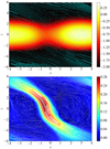Fig. 2. Example of a ring and gap structure and its surrounding outflow topology in the 3D shearing box simulation of Riols & Lesur (2018) with ambipolar diffusion. Top panel: gas density (colourmap in log scale) and streamlines (cyan lines) in the poloidal plane (x and z are respectively the radial and vertical coordinates). Bottom panel: vertical magnetic field (colourmap) and poloidal magnetic field lines (in white) showing the inclined “plume” structure from where most of the mass is extracted. The thickness of the lines is proportional to the field intensity.

2.3. The key role of wind plumes

Another important and recurrent feature of the ring structure is related to the radial velocity profile. Figure 3 shows that the averaged v_x within the midplane (|z|≲H) is opposed to the formation of the ring. In particular, it is anti-correlated with the azimuthal velocity perturbation (zonal flow) and phased with an angle of π/2 with respect to the density maximum. During the ring formation, the matter is thus radially dragged towards the gap in average. Physically, this is expected since the turbulent stress acts like an effective viscosity that tends to diffuse any density bulge in the disc. Therefore, the only way to produce a ring is through vertical transport of matter. We find that the strong wind plume identified in Fig. 2 indeed clear out the gas in the gap regions. In other words, the ring structure does not result from matter being radially concentrated but from material in the gaps being depleted. We note that a similar result is obtained for other magnetisations and in larger box simulations with more than one ring. A detailed mass budget is provided in Appendix D for such simulation. In the next section, we show that a wind-driven instability is probably connected with the formation of these plumes, which organise the flow into radial sub-structures.

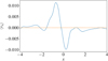Fig. 3. Radial velocity computed from the 3D simulation of Fig. 2. It is averaged in the azimuthal direction, in z within ±1.5H and during the first 50 orbits (∼300 Ω−1), corresponding to the growth of the ring structure.

3. A unified theory based on a wind instability

3.1. Naive picture of the instability

Here we set out the basic principles of a wind instability, that may lead to the growth of ring structures in accretion discs. To start with, consider a classical “α” disc with constant and uniform viscosity ν_t = αc_sH. Assume initially a small axisymmetric and radial perturbation of the surface density δΣ. In the local approximation, then the viscous stress generates a radial flow associated with angular momentum transport,

$$\begin{array}{c}\hfill \delta v_{\mathrm{R}}=-{\displaystyle \frac{2{\nu }_{\mathrm{t}}}{\mathrm{\Sigma }}}{\displaystyle \frac{\partial \delta \mathrm{\Sigma }}{\partial R}},\end{array}$$(1)

which acts to diffuse the initial density ring perturbation. This is a classical and trivial result of the viscous disc theory. In the absence of winds, the perturbation decays and the disc remains stable. If now we include a wind, associated with a large-scale poloidal magnetic field that removes the mass and angular momentum, the outcome may be radically different and potentially lead to an instability. In Fig. 4 we sketch out the main dynamical ingredients of such instability. If the magnetic diffusivity is not too high, the radial flow generated by the viscous stress concentrates the vertical magnetic flux B_z in the density minima or gaps (green patches). Because matter and magnetic flux are transported radially at the same speed δv_R, we expect the magnetisation $\mu \propto B_z^2/(\Sigma c_{\text{s}}\Omega )$ to increase within the density minima. In such circumstances, the wind that was originally uniformly distributed in R, will adjust to this new configuration. A key hypothesis is that the vertical mass flux of the wind ${\dot{\sigma }}_{\mathit{w}}$ (proportional to the surface density) increases with μ. Therefore, if the magnetised gaps eject more material than viscosity can bring in, the initial perturbation is reinforced.

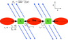Fig. 4. Sketch illustrating the development of rings in accretion discs. The black and blue arrows represent the radial flow and the wind, respectively. The green patches correspond to density minima where the vertical field Bz and the magnetisation μ grow. In this representation, the poloidal field lines (// to the wind) do not bend in the midplane but cross the disc with some angle. This configuration is actually not intuitive but is encountered in various disc simulations around the midplane.

Quantitatively, an instability occurs whenever the surplus of mass launched in the wind is larger than the mass flowing radially. If we note r_a the typical separation between the rings and $p=dlog{\dot{\sigma }}_{\mathit{w}}/d\mu >0$, the instability criterion becomes

$$\begin{array}{c}\hfill r_a{\dot{\sigma }}_w[2p{\displaystyle \frac{\delta B_z}{B_z}}-(p-1){\displaystyle \frac{\delta \mathrm{\Sigma }}{\mathrm{\Sigma }}}]>\mathrm{\Sigma }\delta v_{\mathrm{R}}.\end{array}$$

Using relation (1) and the transport equation for B_z, it is possible to show that the instability criterion is simply p >  0. In sum, the instability is driven by the combination of an outflow and a radial flux transport, and appears optimal in the ideal limit. Rings do not originate from a radial concentration of matter but result from the vertical depletion of their surrounding gaps. The instability is of same nature as Lubow et al. (1994) and Cao & Spruit (2002) but does not require a wind torque (this point is discussed in Sect. 6). We note that the radial pressure gradient associated with the rings has to be balanced by the Coriolis force. The geostrophic equilibrium naturally gives birth to a zonal flow with v_ϕ >  v_K in the regions where v_R <  0 and v_ϕ <  v_K where v_R >  0 (see Fig. 4).

Although the instability mechanism relies on simple physical arguments, it needs to be demonstrated rigorously through a linear analysis of the MHD equations. Moreover there are many caveats to the simple picture described here: first the viscosity or transport coefficient α generally depends on μ, which is a widely accepted result based on turbulent MHD simulations. This effect may reduce the strength of the instability. Second, it is unclear what happens if angular momentum is free to flow along the poloidal magnetic field line. The presence of a mean toroidal field and a vertical stress could in principle have important consequences on the re-distribution of angular momentum. Finally, we do not yet know how the instability behaves if the disc is subject to magnetic diffusion and non-ideal effects. In the next section, we derive a general instability criterion taking into account several of these effects.

3.2. Averaged equations in the local framework

To simplify the problem, we have used the local shearing sheet framework (Goldreich & Lynden-Bell 1965). This corresponds to a Cartesian patch of the disc, centred at r = R₀, where the Keplerian rotation is approximated locally by a linear shear flow plus a uniform rotation rate Ω = Ω e_z. We note (x, y, z) the radial, azimuthal and vertical directions respectively.

To analyse the radial disc structure, we azimuthally and vertically integrated the equations of motion and therefore neglected the vertical dependence of the flow. For that purpose, we introduced two average procedures in the plane (y, z): a standard average $⟨\underline{·}⟩$ between −z_d and z_d, where z_d is some arbitrary altitude, and a mass-weighted average $\overline{·}$ so that for any field φ, we have:

$$\begin{array}{c}\hfill ⟨\phi ⟩(x)={\displaystyle \frac{1}{L_y}}{\displaystyle \int {\int }_{-z_d}^{z_d}\phi }\mathrm{d}z\mathrm{d}y\text{and}⟨\underline{\phi }⟩=⟨\phi ⟩/(2z_d),\end{array}$$

$$\begin{array}{c}\hfill \overline{\phi }(x)={\displaystyle \frac{1}{L_y\mathrm{\Sigma }}}{\displaystyle \int {\int }_{-z_d}^{z_d}\rho \phi }\mathrm{d}z\mathrm{d}y,\end{array}$$

where ρ is the fluid density and $\Sigma (x)=<\rho >=\int {\int }_{-z_d}^{z_d}\rho \hspace{0.17em}\text{d}z\text{d}y$ the surface density. Each field can be decomposed into a sum of a mean component (depending on x only) and a fluctuation

$$\begin{array}{c}\hfill \phi =\overline{\phi }(x)+\phi \prime (x,y,z)\text{or}\phi =⟨\underline{\phi }⟩(x)+\delta \phi (x,y,z).\end{array}$$(2)

We also note $[{\dot{]}}_{-}^{+}$ the difference between the field at z = z_d and z = −z_d. The compressible, inviscid and isothermal equations of motion in the horisontal plane, integrated azimuthally and vertically between −z_d and z_d are

$$\begin{array}{c}\hfill {\displaystyle \frac{\partial \mathrm{\Sigma }}{\partial t}}+{\displaystyle \frac{\partial }{\partial x}}\left(\mathrm{\Sigma }{\overline{v}}_x\right)+{\dot{\sigma }}_w={\dot{\sigma }}_i,\end{array}$$(3)

$$\begin{array}{c}\hfill {\displaystyle \frac{\partial \mathrm{\Sigma }{\overline{v}}_x}{\partial t}}+{\displaystyle \frac{\partial }{\partial x}}\left(\mathrm{\Sigma }{\overline{T}}_{\mathit{xx}}\right)+W_{\mathit{xz}}-2\mathrm{\Omega }\mathrm{\Sigma }{\overline{v}}_y+c_{\mathrm{s}}^2{\displaystyle \frac{\partial \mathrm{\Sigma }}{\partial x}}+{\displaystyle \frac{\partial }{\partial x}}{\displaystyle \frac{⟨B^2⟩}{2}}=0,\end{array}$$(4)

$$\begin{array}{c}\hfill {\displaystyle \frac{\partial \mathrm{\Sigma }{\overline{v}}_y}{\partial t}}+{\displaystyle \frac{\partial }{\partial x}}\left(\mathrm{\Sigma }{\overline{T}}_{\mathit{yx}}\right)+W_{\mathit{yz}}+{\displaystyle \frac{1}{2}}\mathrm{\Omega }\mathrm{\Sigma }{\overline{v}}_x=0,\end{array}$$(5)

where ${\dot{\sigma }}_{\mathit{w}}={\left[\rho {\mathit{v}}_z\right]}_{-}^{+}$ is the mass loss rate, ${\overline{T}}_{\mathit{ij}}=\overline{{\mathit{v}}_i{\mathit{v}}_j}-\overline{B_i{B}_j/\rho }$ the stress tensor integrated in the vertical direction and $W_{\mathit{ij}}={[\rho {\mathit{v}}_i{\mathit{v}}_j-B_i{B}_j]}_{-}^{+}$ its boundary value. We assumed that mass is replenished locally at a constant rate ${\dot{\sigma }}_i$ (associated with the radial accretion in a global view, which is absent in the local shearing box framework).

These equations of motions are coupled with the induction equation that describes the evolution of the magnetic field B. We are particularly interested in the evolution of the vertical magnetic flux ⟨B_z⟩:

$$\begin{array}{c}\hfill {\displaystyle \frac{\partial ⟨B_z⟩}{\partial t}}={\displaystyle \frac{\partial }{\partial x}}⟨{\mathcal{E}}_y⟩+\eta ({\displaystyle \frac{{\partial }^2}{\partial x^2}}⟨B_z⟩+{\left[{\displaystyle \frac{\partial B_z}{\partial z}}\right]}_{-}^{+}),\end{array}$$(6)

where ℰ_y = v_zB_x − v_xB_z is the toroidal electromotive force and η is assumed to be a constant and uniform ohmic resistivity. An additional constraint is the solenoidal condition which gives

$$\begin{array}{c}\hfill {\displaystyle \frac{\partial ⟨B_x⟩}{\partial x}}+{\left[B_z\right]}_{-}^{+}=0.\end{array}$$

3.3. Stress tensor and electromotive force

We first develop the terms related to the stress tensor ${\overline{T}}_{\mathit{ij}}$ and W_ij. In the limit of highly sub-sonic fluctuations, it is straightforward to show that the radial stress $\mathrm{\Sigma }{\overline{T}}_{\mathit{xx}}$ and the vertical stress in the radial momentum equations are negligible compared to thermal pressure. Thus we can assume that ${\overline{T}}_{\mathit{xx}}\simeq 0$ and W_xz ≃ 0. In the azimuthal momentum equation, however, the stress is comparable to others terms. By using the decomposition of Eq. (2), we have

$$\begin{array}{c}\hfill \mathrm{\Sigma }{\overline{T}}_{\mathit{yx}}=\mathrm{\Sigma }\overline{v_x{v}_y}-⟨B_x{B}_y⟩=({\alpha }_{\nu }+{\alpha }_{\mathrm{L}})\mathrm{\Sigma }{c}_{\mathrm{s}}^2,\end{array}$$(7)

where

$${\alpha }_{\nu }=\frac{\langle \rho v_x^{\prime }{v}_y^{\prime }-\delta B_x\delta B_y\rangle }{\Sigma c_{\text{s}}^2}\text{\hspace{1em} and\hspace{1em}}{\alpha }_{\text{L}}=\frac{\Sigma \overline{v_x}\overline{v_y}-\langle B_x\rangle \langle \underset{\_}{B_y}\rangle }{\Sigma c_{\text{s}}^2},$$

can be identified respectively as a turbulent and laminar radial transport coefficient. The term related to the vertical stress W_yz can be written as

$$\begin{array}{c}\hfill W_{\mathit{yz}}={\alpha }_W\mathrm{\Sigma }{c}_{\mathrm{s}}\mathrm{\Omega }+{\overline{v}}_z{\left[v_y^{\prime }\right]}_{-}^{+}+{\overline{v}}_y{\left[v_z^{\prime }\right]}_{-}^{+}-⟨\underline{B_y}⟩{\left[\delta B_z\right]}_{-}^{+}-⟨\underline{B_z}⟩{\left[\delta B_y\right]}_{-}^{+},\end{array}$$(8)

where ${\alpha }_W=\frac{{\left[\rho v_y^{\prime }{v}_z^{\prime }-\delta B_y\delta B_z\right]}_{-}^{+}}{\Sigma c_{\text{s}}\Omega }$ is the turbulent vertical transport. Finally the electromotive force in Eq. (6) can also be decomposed into a laminar and a turbulent part, the latter being assumed to behave as an effective magnetic diffusivity η_t:

$$\begin{array}{c}\hfill ⟨{\mathcal{E}}_y⟩=⟨\underline{v_z}⟩⟨B_x⟩-⟨\underline{v_x}⟩⟨B_z⟩+{\eta }_{\mathrm{t}}{\displaystyle \frac{\partial ⟨B_z⟩}{\partial x}}\end{array}$$

3.4. Power laws for mass loss rate and turbulent coefficients

To close the system of equations we need to relate the mass loss efficiency $\zeta =\dot{{\sigma }_{\mathit{w}}}/(\mathrm{\Sigma }{\mathrm{\Omega }}^{-1})$ and the turbulent coefficient α_ν, α_W, η_t to the integrated disc quantities. It is reasonable to assume that these coefficients depend principally on the main dimensionless parameter of the disc, namely the vertical magnetisation μ. We suppose that this dependence can be captured by a simple power law:

$$\begin{array}{c}\hfill \zeta ={\displaystyle \frac{\dot{{\sigma }_w}}{\mathrm{\Sigma }{\mathrm{\Omega }}^{-1}}}={\zeta }_0{\left({\displaystyle \frac{\mu }{{\mu }_{\mathrm{eq}}}}\right)}^p\end{array}$$

$$\begin{array}{c}\hfill {\alpha }_{\nu }={\alpha }_{{\nu }_0}{\left({\displaystyle \frac{\mu }{{\mu }_{\mathrm{eq}}}}\right)}^q\end{array}$$

and similar relations for α_W and η_t. μ_eq, ζ₀ and α_ν0 correspond to values of a given equilibrium (see next section). Numerical simulations are actually a suitable tool to probe and test these scaling laws. The dependence of α_ν on the magnetisation has been explored in various ideal simulations of MRI turbulence, with or without magnetic diffusion and thermal effects (Hawley et al. 1995; Simon et al. 2013; Salvesen et al. 2016; Scepi et al. 2018). In all cases, there is some consensus that

$$\begin{array}{c}\hfill q\simeq 0.5\text{for}\mu \gtrsim {10}^{-5}.\end{array}$$

The vertical transport due to a wind has also been measured in simulations (Bai & Stone 2013; Fromang et al. 2013; Zhu & Stone 2018; Scepi et al. 2018) but is generally supplied by a large scale toroidal field instead of turbulent fields. Properly characterising α_W would require us to measure the laminar and turbulent contribution of the stress separately, which has never been done in the literature. The turbulent diffusivity has been calculated in 3D unstratified shearing box simulations (Guan & Gammie 2009; Fromang & Stone 2009; Lesur & Longaretti 2009) and a fair assumption is to consider η_t between 0.2 and 0.5ν_t (where ν_t = α_νc_sΩ). However, we see in Sect. 4 that such a ratio can actually be much weaker in 2D. Finally, evaluating the mass loss rate is probably the hardest part since it depends on the vertical box size and the nature of boundary conditions (Fromang et al. 2013). Simulations of 1D laminar winds predict p ≈ 0.6−0.7 (see Fig. 4 of Riols et al. 2016) while full 3D turbulent simulations suggest p ≃ 1; see Fig. 5 of Suzuki & Inutsuka (2009) and Fig. 4 of Scepi et al. (2018).

3.5. Local equilibrium solutions

We use a sub-script “0” to indicate the equilibrium solutions (independent of time and x) of the system of equations derived in Sect. 3.2. The local disc equilibria are obtained by setting ∂⋅/∂t = 0 and ∂⋅/∂x = 0 in Eqs. (3)–(6). We note that in absence of turbulence, these equilibria correspond to the vertical average of the 1D (z-dependent) wind solutions studied by Lesur et al. (2013) and Riols et al. (2016). The solenoidal condition gives immediately δB_z = 0, which means that $B_z=⟨\underline{B_z}⟩=B_{z_0}$. We can then define a constant magnetisation of the equilibrium, as

$$\begin{array}{c}\hfill {\mu }_{\mathrm{eq}}=\sqrt{{\displaystyle \frac{\pi }{2}}}{\displaystyle \frac{B_{z_0}^2}{{\mathrm{\Sigma }}_0{c}_{\mathrm{s}}\mathrm{\Omega }}}·\end{array}$$

Solutions can be either symmetric about the midplane with B_x = B_y = 0 at z = 0 or anti-symmetric with ∂_zB_x = ∂_zB_y = 0.

1. In the symmetric case, we have ⟨B_x⟩ = ⟨B_y⟩ = 0 but ${\overline{\mathit{v}}}_x,{\overline{\mathit{v}}}_{\mathit{y}}\ne 0$. Horizontal components satisfy ${[\mathit{v}\prime ]}_{-}^{+}=0$ but ${\left[\delta b\right]}_{-}^{+}\ne 0$. Therefore there is a net vertical stress through the disc, which is responsible for a mean accreting flow.

2. In the second case ⟨B_x⟩ = ⟨B_y⟩≠0 but ${\overline{\mathit{v}}}_x,{\overline{\mathit{v}}}_{\mathit{y}}=0$. We define B_x0 and B_y0 the mean radial and toroidal magnetic field throughout the midplane. Departures to the vertical average satisfy ${[{\mathit{v}}_{x,\mathit{y}}\prime ]}_{-}^{+}\ne 0$ but ${\left[\delta b\right]}_{-}^{+}=0$. It is straightforward to check that W_yz0 = 0 when such symmetry is enforced.

Historically, the first class of solutions (1) were considered to be the most intuitive and representative of a disc structure; the reason being that magnetic field lines do not bend outside the midplane. However anti-symmetric solutions have been shown to naturally emerge from turbulent shearing box simulations (Lesur et al. 2014; Bai 2015), and even from global simulations when non-ideal effects are included (Béthune et al. 2017; Bai 2017). For that reason, we focus mainly on the anti-symmetric solutions in the following sections.

3.6. Linearisation around equilibrium

We use the sub-script “0” to indicate equilibrium solution of Eqs. (3)–(6) enforcing the second class of symmetry. We remind the reader that such symmetry implies that ${\overline{\mathit{v}}}_0=0$ at equilibrium. To study the stability of these solutions, we introduce small normalised axisymmetric perturbations of the form $\widehat{\phi }\propto exp(i{k}_{x}x+\sigma t)$ around the equilibrium flow:

$$\begin{array}{c}\hfill \mathrm{\Sigma }={\mathrm{\Sigma }}_0(1+\widehat{\mathrm{\Sigma }});\overline{v_x}=\widehat{u}{c}_{\mathrm{s}};{\overline{v}}_y=\widehat{v}{c}_{\mathrm{s}};⟨B⟩=B_0(1+\widehat{b}).\end{array}$$

We can perform a similar decomposition for the magnetisation

$$\begin{array}{c}\hfill \mu ={\mu }_{\mathrm{eq}}(1+\widehat{\mu })={\mu }_{\mathrm{eq}}(1+2{\widehat{b}}_z-\widehat{\mathrm{\Sigma }})\end{array}$$

as well as the turbulent coefficients and mass loss rate whose first order perturbation is proportional to $\widehat{\mu }$. To be consistent with the formalism of Sect. 3.2, the radial scale of perturbations is supposed to be much larger than the turbulent lengthscale. Because turbulent eddies are, in principle, limited to the disc scale height, we have considered modes with k_xH ≲ 1 and assume σ ≪ Ω. To simplify the problem, we made the following further assumptions:

1. Perturbations are in a geostrophic equilibrium (pressure gradient balances Coriolis force in the x direction). This is satisfied if σ ≪ Ω.

2. The vertical component of the Reynolds stress tensor ${\overline{v}}_z{\left[v_y^{\prime }\right]}_{-}^{+}+{\overline{v}}_y{\left[v_z^{\prime }\right]}_{-}^{+}$ as well as the turbulent vertical stress α_W = 0 are neglected

3. The stress is purely turbulent α_ν0 ≫ α_Ł0

4. In Eq. (6), the vertical stretching of radial field ⟨u_z⟩⟨B_x⟩ and the vertical diffusion of B_z are neglected.

5. We have assumed that $⟨\underline{{\mathit{v}}_x}⟩\simeq {\overline{\mathit{v}}}_x$. This is true if the radial velocity perturbation does not vary too much between -z_d and z_d.

Some of these assumptions are tested in simulations (see Appendices C and D). A more general case, including a laminar stress and a departure from the geostrophic equilibrium due to a strong toroidal field, is treated in Appendix B. By using these hypothesis, we show that the linearised momentum transport due to the total stress at leading order simply reduced to

$$\begin{array}{c}\hfill {\displaystyle \frac{\partial }{\partial x}}\left(\mathrm{\Sigma }{\overline{T}}_{\mathit{yx}}\right)+W_{\mathit{yz}}=i{k}_x{\alpha }_{{\nu }_0}[\widehat{\mathrm{\Sigma }}+q\widehat{\mu }]{\mathrm{\Sigma }}_0{c}_{\mathrm{s}}^2.\end{array}$$

We note that the perturbation of vertical stress cancels out with the term –$⟨B_{\mathit{y}}⟩⟨\underline{B_x}⟩{\widehat{b}}_x$ in the azimuthal momentum equation (see Appendix A). We normalised k_x to H and σ to Ω and define η^⋆ = (η + η₀)/(H²Ω). Linearisation of Eqs. (3)–(6) around equilibrium leads to

$$\begin{array}{c}\hfill \sigma \widehat{\mathrm{\Sigma }}+i{k}_x\widehat{u}+p{\zeta }_0\widehat{\mu }+{\zeta }_0\widehat{\mathrm{\Sigma }}=0\end{array}$$(9)

$$\begin{array}{c}\hfill -2\widehat{v}+i{k}_x\widehat{\mathrm{\Sigma }}=0,\end{array}$$(10)

$$\begin{array}{c}\hfill \sigma \widehat{v}+i{k}_x{\alpha }_{{\nu }_0}(q\widehat{\mu }+\widehat{\mathrm{\Sigma }})+{\displaystyle \frac{1}{2}}\widehat{u}=0,\end{array}$$(11)

$$\begin{array}{c}\hfill \sigma {\widehat{b}}_z+i{k}_x\widehat{u}=-{\eta }^{\star }{k}_x^2{\widehat{b}}_z.\end{array}$$(12)

3.7. Stability criterion and growth rates

The linear system of Eqs. (9)–(12) can be simplified and cast into a (3 × 3) matrix problem whose determinant is

$$\begin{array}{c}\hfill D=\left|\begin{array}{ccc}\sigma +{\zeta }_0& i{k}_x& p{\zeta }_0\\ {\displaystyle \frac{\sigma }{2}}+{\alpha }_{{\nu }_0}& -{\displaystyle \frac{i}{2k_x}}& {\alpha }_{{\nu }_0}q\\ \sigma +{\eta }^{\star }{k}_x^2& 2i{k}_x& \sigma +{\eta }^{\star }{k}_x^2\end{array}\right|.\end{array}$$(13)

Solutions of the problem are found by setting D = 0. It is straightforward to show that growth rates follow the dispersion relation

$$\begin{array}{c}\hfill A{\sigma }^2+B\sigma +C=0\end{array}$$(14)

with

$$\begin{array}{cc}\hfill A& =1+k_x^2\hfill \\ \hfill B& =2k_x^2{\alpha }_{{\nu }_0}(1+q)-{\zeta }_0(p-1+2p{k}_x^2)+{\eta }^{\star }[k_x^2+k_x^4]\hfill \\ \hfill C& =-4{\zeta }_0{k}_x^2{\alpha }_{{\nu }_0}(p-q)+{\eta }^{\star }{k}_x^2[{\zeta }_0(1-p)+2{\alpha }_{{\nu }_0}(1-q)k_x^2].\hfill \end{array}$$

There are actually two different regimes, depending on the strength of the turbulent stress. The first one corresponds to B <  0, i.e α_ν0 ≪ ζ₀ and $k_x^2>(1-p)/(2p)$). In that regime, solutions are always unstable (ℜ(σ) > 0). The radial flow that concentrates magnetic flux is directly produced by the inertial term $\sigma \widehat{v}$, via the geostrophic equilibrium and the conservation of angular momentum. However, this particular regime, though quite exotic and allowing the instability for α = 0, is never encountered in simulations. The second regime corresponds to B >  0 or α_ν0 ≫ ζ₀. In that case, the instability occurs if C <  0, which corresponds in the ideal limit (η^⋆ = 0), to

$$\begin{array}{c}\hfill p>q.\end{array}$$

If p <  1 and q <  1, the non-ideal term in C is always positive. Therefore it contributes to weaken the growth rate. We note that the hypothetical case q >  1 and p = ζ₀ = 0 (no winds) can in principle lead to an instability in presence of finite resistivity but is excluded by the simulations. It corresponds to the usual, but hypothetical “viscous” instability, like imagined by Lightman & Eardley (1974).

In the ideal limit (η^⋆ = 0), it is straightforward to show that the optimal growth rate is obtained in the limit k_x ≫ 1. Under the condition α_ν0 ≫ ζ₀, which is verified in most of simulations, it can be demonstrated that the optimal growth rate, at leading order, is independent of α_ν0 and proportional to ζ₀:

$$\begin{array}{c}\hfill \sigma \simeq 2{\zeta }_0\left({\displaystyle \frac{p-q}{1+q}}\right).\end{array}$$

For typical MRI-driven turbulence with μ_eq = 10⁻³, realistic values of the parameters are α_ν ≃ 0.3, p ≃ 1, q ≃ 0.5 and ζ₀ ≃ 0.01. Using these values, we find in the ideal limit σ = 0.00666. To illustrate the effect of magnetic diffusivity, we plot in Fig. 5 the growth rate of the instability σ as a function of k_x for three different resistivities (η^⋆ ≃ 0.002, 0.01, 0.06). These values are here purely ad-hoc and just to illustrate the dependence of σ(k_x) on η^⋆. Realistic values, directly inferred from 2D and 3D simulations, are used in Sects. 4 and 5. In all cases, the maximum growth rate is obtained for k_xH ≲ 0.5H which correspond to rings of size r_a ≳ 10 H. The instability occurs on long timescale 1/σ larger than 150 Ω⁻¹ (20 orbits).

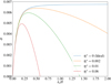Fig. 5. Growth rate of the wind-driven instability as a function of the radial wavenumber for different magnetic diffusivities. Parameters of the model have been chosen in agreement with numerical simulations for fiducial μeq = 10−3: αν ≃ 0.3, p ≃ 1, q ≃ 0.5, ζ0 ≃ 0.01.

3.8. Eigenmodes

The linearised system admits solutions of the form:

$$\begin{array}{c}\hfill \left(\begin{array}{c}\widehat{u}\\ \widehat{v}\\ {\widehat{b}}_z\end{array}\right)=\left(\begin{array}{c}-i{k}_{x}E\\ i{k}_x/2\\ -k_x^{2}E/(\sigma +{\eta }^{\star }{k}_x^2)\end{array}\right)\widehat{\mathrm{\Sigma }},\end{array}$$(15)

with $E=\left[(\sigma /2+{\alpha }_{{\nu }_0})p{\zeta }_0-{\alpha }_{{\nu }_0}q({\zeta }_0+\sigma )\right]/(p{\zeta }_0/2+k_x^2{\alpha }_{{\nu }_0}q)$ a small number compared to 1. In the turbulent regime with α_ν ≫ ζ, and if p >  q, it is straightforward to show that E >  0. The radial velocity perturbation is out of phase (with an angle of π/2) with respect to the density maximum and anti-correlated with the zonal flow $\widehat{\mathit{v}}$. The vertical field and the magnetisation are anti-correlated with the density maximum. This configuration is exactly that depicted in Sect. 2.

4. 2D axisymmetric simulations

To test our instability model, we needed to confront the theoretical predictions of Sect. 3 with MHD numerical simulations exhibiting rings structures. As a preliminary check, we performed in Appendix C a stability analysis around an initial laminar wind equilibrium, using 2D shearing box simulations. We find that axisymmetric perturbations undergo clean exponential growth with rates and eigenfunctions compatible with our theory. In this section, we explore the case of a turbulent disc, by using 2D simulations initialised with a net vertical field and random noise. In particular, we check whether the numerical growth rate and spacing of axisymmetric modes, as well as their physical behaviour, are compatible with the linear theory.

4.1. Numerical setup

Shearing-box simulations were run with the PLUTO code (Mignone et al. 2007), a finite-volume method with a Godunov scheme that integrates the compressible MHD equations in their conservative form. The fluxes are computed with the HLLD Riemann solver for runs without ambipolar diffusion and with HLL otherwise. The gas is isothermal and inviscid (no explicit viscosity). Boundary conditions are shear-periodic in x and periodic in y. In the vertical direction, we used standard outflow boundary conditions for the velocity field and imposed hydrostatic balance in the ghost cells for the density. In this way, we significantly reduced the excitation of artificial waves near the boundary. For the magnetic field, we used the “vertical field” or open boundary conditions with B_x = 0 and B_y = 0 at z = ±L_z/2. Because the instability we seek occurs on a long timescale, it is important to maintain a constant disc surface density Σ. Otherwise, the wind would empty the disc before the instability reaches any saturated state. For that purpose, we regularly injected mass near the midplane at each numerical time step. The source term in the mass conservation equation is similar to the one prescribed by Lesur et al. (2013),

$$\begin{array}{c}\hfill {\dot{\sigma }}_i={\displaystyle \frac{2\dot{{\rho }_i}(t)}{\sqrt{2\pi }{z}_i}}exp(-{\displaystyle \frac{z^2}{2z_i^2}}),\end{array}$$(16)

where $\dot{{\rho }_i}(t)$ is the mass injection rate computed at each time step to maintain the total mass constant in the box, and z_i is a free parameter that corresponds to the altitude below which mass is replenished. We note that σ_i is uniformly distributed in x and y and thus independent of local density variations in the box.

For most of the simulations, we chose a large horizontal box size L_x = L_y = 20 H to be able to capture the largest rings. In z, the box spans −4 H to 4 H. We adopted a resolution of 256 points in the horizontal directions and 128 points in the vertical direction. In the ideal regime, such a resolution is insufficient to resolve the small-scale MRI turbulence properly, but enough to obtain the right axisymmetric dynamics. We checked that doubling resolution (512 × 256) does not change the results in terms of growth rate and spacing.

Finally, for simulations with ambipolar diffusion, we use exactly the same setup as Riols & Lesur (2018) where the ambipolar Elsasser number Am is one in the midplane, and increases abruptly above a certain height corresponding to the FUV ionisation layer (see Sect. 2.4 of the paper for further detail of the prescription and its physical motivation).

4.2. Simulations in the ideal limit and numerical growth rates

We first run a series of 2D axisymmetric simulations in the ideal limit (without explicit resistivity or ambipolar diffusion) by varying the vertical magnetisation μ_eq from 10⁻⁵ to 0.03. All runs are initialised with a hydrostatic equilibrium in density and a weak random noise in velocity. Figure 6 shows the evolution of the turbulent and laminar transport coefficients α_ν, α_L and the wind loss efficiency ζ for the case μ_eq = 10⁻³. To complement the analysis, the evolution of column density Σ(x) is illustrated in Fig. 7 (top panels) for three different magnetisation μ_eq = 10⁻⁴, 10⁻³ and 10⁻². Each quantity is integrated between −1.5 and 1.5 H. In all cases, we identify three distinct phases associated with: (a) the development of vigorous MHD turbulence and the launching of a wind during the first ∼50−150 Ω⁻¹, (b) the growth of zonal flows and density rings, and c) the saturation of zonal flows which is accompanied by a severe drop in the turbulent stress and a modest drop in the wind loss efficiency ζ (see Fig. 6). We note that during the initial turbulent phase, α_ν ≫ α_L, while after the saturation of sub-structures, the radial stress is predominantly laminar α_ν ≪ α_L. Figure 7 shows that the timescale associated with rings formation seems to decrease with μ_eq while their spacing and strength seems to increase with μ_eq.

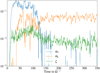Fig. 6. Evolution of the transport coefficient αν, αL and the wind mass loss efficiency ζ in the 2D simulation without explicit diffusion (μeq = 10−3)

Fig. 7. Top: space-time diagram showing the column density as a function of time and x, in 2D axisymmetric turbulent simulations, for different magnetisation (left to right, μeq = 10−4,  10−3 and 10−2). The density is integrated within z ± 1.5H and runs were computed in the ideal limit (without explicit magnetic diffusion). Bottom panels: for each run, time-evolution of ${\widehat{b}}_z$, normalised projection of Bz onto the prominent axisymmetric Fourier mode (with largest amplitude). This mode corresponds respectively to kx = 6, 4 and 2kx0 for μeq = 10−4,  10−3 and 10−2, with kx0 = 2π/Lx the fundamental box radial wavenumber.

To understand whether rings form via a linear instability or a more complicated non-linear process, we explored the dynamics of axisymmetric modes in Fourier space. The procedure is simple: at each time-step, we perform a 1D FFT (along the x direction) of the vertically averaged quantities. We then project each field (or any physical quantity) onto the dominant axisymmetric mode that grows during the simulation¹. In this way, we keep the interesting dynamics related to the prominent ring and filter out part of the dynamics associated with the turbulent flow. For a given field φ, we note $\widehat{\phi }$ such projection, normalised with respect to its mean (the k_x = 0 mode in Fourier space).

The bottom panels of Fig. 7 show the evolution of ${\widehat{b}}_z$ for three different magnetisations. In all cases, the prominent ring mode begins to grow quasi-exponentially, indicating that a linear instability is at work. We note that the projection procedure is necessary to obtain a clean exponential growth at the beginning of simulations. After a few tens of orbits, the growth stops and ${\widehat{b}}_z$ saturates around one. This is an indication that a non-linear regime is reached.

During the linear phase, we measure the growth rates associated with the prominent mode and report them in Fig. 8 for different μ_eq. For μ_eq >  10⁻⁴, growth rates increase with the magnetisation and vary from 0.002 to 0.05 Ω; the dependence of σ with μ_eq follows a power law with index 0.7−0.8. We checked that σ is not changed when doubling the resolution of simulations. It is worth noting that such growth rates are ∼10−20 smaller than those characterising the MRI at a similar scale.

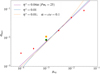Fig. 8. Optimal growth rate of the instability as a function of the magnetisation μ. The red diamond markers are the growth rates of the most unstable Fourier mode measured in 2D ideal simulations. The orange and green crosses are those measured in resistive and ambipolar runs. The purple solid line correspond to the model prediction, using the scaling relations (17) and (18). The blue and yellow dashed lines use the same model but with constant η⋆ = 0.01 in both cases and constant αν = 0.1 for the last case.

4.3. Non-ideal case

We first investigated the effect of ohmic resistivity on the growth of axisymmetric structures. For that, we ran a 2D simulation with μ_eq = 10⁻³ and explicit η/(ΩH²) = 0.01. This corresponds to a magnetic Reynolds number Rm = ΩH²/η = 100. During the first tens of orbits, a turbulent state develops but with a much weaker strength and transport than in the ideal case (for comparison, α ≃ 0.05). Such a result is expected since the MRI is quenched by the resistivity. However, the wind mass loss efficiency ζ is of the same order of magnitude. Three rings, associated with a mode k_x = 3k_x0 develop in the box and grow at a rate σ ≃ 0.011Ω. The number of rings, their properties, and the growth rate are actually comparable to those obtained in the ideal case.

We then studied the effect of ambipolar diffusion by running a simulation with the same μ_eq = 10⁻³ and Am = 1 in the midplane. Figure 9 shows the evolution of surface density and vertically-averaged B_z. Again three or four structures seem to emerge from the initial turbulent phase. The growth rate associated with the k_x = 4k_x0 mode in Fourier space is σ ≃ 0.0085, very similar to the value obtained in the ideal limit. Thus, ambipolar diffusion does not seem to alter the instability mechanism, although it weakens or even suppresses the initial turbulent state.

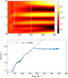Fig. 9. Top panel: space-time diagrams showing the surface density Σ(x, t) in the 2D ambipolar simulation (Ammid = 1, μeq = 10−3 and zd = 2H). The two vertical dashed lines delimit the “linear” phase, during which zonal modes, in Fourier space, grow exponentially. Bottom panel: evolution of the Bz component projected onto the kx = 4kx0 mode.

We note that contrary to the ideal case, the turbulent transport is either comparable to or smaller than the laminar transport α_L. To go further in the analysis and check that the instability identified numerically is of same nature as that described in Sect. 3, we inspected in the ambipolar run the different flux and source terms in Eqs. (3)–(6). For ease of reading, this analysis is presented in Appendix D. We show in particular that the ambipolar term η_AJ × (B × B)/B² merely acts as a diffusion on the B_z field.

4.4. Parameters p and q and confrontation with the model

In this section, we describe our investigation of whether the dependence of numerical growth rates σ(μ_eq) can be predicted by the simple model exposed in Sect. 3. We have focussed particularly on the ideal simulations, for which α_L0 ≪ α_ν0 during the linear phase. The linear theory can actually be generalised to quasi-laminar discs with α_L0 ≳ α_ν0 (see Appendix B), typically those obtained in non-ideal simulations. The instability in this regime is conceptually not different and the theoretical growth rates are comparable to those obtained with a pure turbulent stress.

The model of Sect. 3 depends on three main parameters p = d log(α_ν)/d log(μ), q = d log(ζ)/d log(μ) and the diffusivity η_⋆. To evaluate these coefficients, it is suitable to measure them directly from numerical simulations. A naive way is to run a series of turbulent simulations varying μ and measuring α_ν, ζ and η_⋆. Though simple, this method is complicated to accomplish in practise. Indeed, as suggested by Fig. 6, the quasi-steady turbulent state obtained in the early stage of simulations is short (< 100 Ω⁻¹) and rapidly affected by the zonal structures. This turns to be particularly critical at large μ_eq, for which measures of transport coefficient and mass loss rate are not statistically meaningful and can be highly inaccurate.

A possible way to circumvent this issue is to infer directly the scaling relations from a thorough inspection of the large-scale ring perturbations themselves. The idea is to compute the perturbed coefficients ${\widehat{\alpha }}_{\nu }$ and $\widehat{\zeta }$ associated with the dominant axisymmetric mode and see how it correlates in time with the perturbed magnetisation $\widehat{\mu }$. In addition to giving p and q, it provides a great opportunity to check the linear relations conjectured in Sect. 3.6, which are fundamental requisites of the instability.

Figure 10 shows the two ratios $p=\widehat{\zeta }/\widehat{\mu }$ and $q={\widehat{\alpha }}_{\nu }/\widehat{\mu }$ for the case μ_eq = 10⁻⁴. Here ${\widehat{\alpha }}_{\nu }$, $\widehat{\zeta }$ and $\widehat{\mu }$ are the vertically averaged perturbations of transport, mass loss efficiency and magnetisation projected onto the Fourier mode k_x = 6 × 2π/L_x and normalised with respect to the mean (k_x = 0 mode). We note that the latter is averaged in time during the growth phase. Although these ratios are highly fluctuating (this is particularly true for p), $\widehat{\zeta }$ and $\widehat{\alpha }$ seem linearly correlated to the magnetisation $\widehat{\mu }$, at least statistically. Most importantly, we check that p >  q. An interesting, but unexpected, result is that the ratios seem to keep a similar value in the saturation regime (t ≳ 500Ω⁻¹). By averaging over time, we find q ≃ 0.4 and p ≃ 0.9 in agreement with the scaling relations obtained in 3D fully turbulent simulations (Scepi et al. 2018). We performed the same calculation for μ_eq = 10⁻³ and found p ≃ 0.8 and q ≃ 0.55.

In summary, we adopted the following scaling laws in our model:

$$\begin{array}{c}\hfill {\alpha }_{\nu }=4{\mu }^{0.45}\text{and}\zeta =4.5{\mu }^{0.8}\end{array}$$(17)

with the constants calibrated to fit with the simulation data at intermediate μ = 10⁻³ (values are taken from Fig. 6). Simulations in this regime generally provide a more accurate measure of α_ν0 and ζ₀ since the turbulent phase settles longer. The dependence of α is very close to that obtained in past 3D simulations (see Eq. (20) of Salvesen et al. 2016).

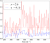Fig. 10. Coefficients p and q measured from the 2D ideal simulation with μeq = 10−4. The red (respectively blue) line shows the ratio between the perturbation of ζ (respectively α) and the perturbation associated with magnetisation, as a function of time. Each quantity (ζ, α and μ) is projected onto the mode kx = 6kx0, averaged within z ± 2H and normalised to its mean.

To estimate the turbulent magnetic diffusivity, we have used a slightly different method. Instead of projecting the flow into the Fourier space, we calculated the averaged term $⟨{\mathcal{E}}_{\mathit{y}}⟩-⟨\underline{{\mathit{v}}_z}⟩⟨B_x⟩+⟨\underline{{\mathit{v}}_x}⟩⟨B_z⟩$ directly in real space during the linear growth of the mode. We checked that it correlates quite well in space with ∂⟨B_z⟩/∂x and indeed acts to diffuse the large scale structure. The ratio between the two terms is η_t/(ΩH²) ≈ 0.003 for μ_eq = 10⁻⁴ and η_t ≈ 0.008 for μ_eq = 10⁻³. This corresponds to rather low turbulent diffusivities, compared to values given by Lesur & Longaretti (2009) in the unstratified 3D case. The turbulent Prandlt number Pm = α_ν/η_t is of order 25 and we checked that it depends little on resolution. Therefore, we consider:

$$\begin{array}{c}\hfill {\eta }_{\mathrm{t}}=0.04{\alpha }_{\nu }.\end{array}$$(18)

These scaling laws are then used as inputs of our model (Sect. 3.7), and allow us to compute the optimal growth rate as a function of μ (using Eq. (14)). The result is superimposed in Fig. 8 (purple curve). The model fits quite well with the numerical values obtained in Sect. 4.2, and in particular reproduces the slope of σ(μ) for intermediate μ. We stress that such a result does not rely exclusively on the linear correlations measured in Fig. 10, since growth rates depend also on the absolute values of ζ. To show that the model is robust, we also plot the theoretical growth rates obtained for a constant magnetic diffusivity (blue curve) and constant α and η^⋆ (yellow dashed curve). In both cases, there are few differences with the prescription η_t = 0.04 α_ν. This is unsurprising since maximum growth rates depend little on α and η^⋆ (for the range of diffusivities considered here, see Fig. 5).

We finally comment on the extreme cases, corresponding to the lowest and highest magnetisations in Fig. 8. In these regimes, the numerical values slightly deviate from the model. For μ ≳ 10^−1.5, measures are perhaps inaccurate since growth rates associated with large-scale modes become comparable to those associated with the MRI phase. For μ ≲ 10⁻⁴, the small discrepancy is probably due to a sudden drop in α and η_t. The fact that the turbulence dies out at low μ is expected since the 2D box does not sustain a dynamo in the limit μ → 0. As turbulent dissipation is weakened, zonal flows are slightly enhanced. This effect, however, remains marginal and only holds for 10⁻⁵ ≲ μ ≲ 10⁻⁴. Below μ = 10⁻⁵, the vertical flux of mass associated with the wind drops abruptly, and we checked numerically that zonal flows vanish.

4.5. Non-linear saturation and ring/gap contrast

As suggested by Fig. 7, the ring instability saturates and enters a non-linear regime, once the azimuthal structures reach a significant amplitude. During this phase, the structures stop growing but prevail in the flow and remain stable for hundreds of orbits. Their non-linear saturation leads to a drop in the mean stress (Fig. 6) and the production of a strong mean azimuthal field B_y, altering significantly the initial hydrostatic density profile. But it is still not clear how this saturation occurs and what determines the final amplitude (or density contrast) of the rings. By examining the density contrast in the case μ = 10⁻⁴ or μ = 10⁻³ (upper panels of Fig. 7), we find that the gaps in the non-linear regime still contain a large amount of gas. For instance, the surface density perturbation associated with the prominent Fourier mode, settles towards $\widehat{\mathrm{\Sigma }}\sim 0.09$ for μ_eq = 10⁻⁴ and $\widehat{\mathrm{\Sigma }}\sim 0.42$ for μ_eq = 10⁻³. Therefore, saturation does not occur because the material in the gaps has been emptied. The lower panels of Fig. 7 show instead that the instability saturates when ${\widehat{b}}_z\sim 1$ (i.e perturbation of B_z ∼ B_z0). In other words, the instability stops when there is no more vertical flux to drag in. The density contrast between the gaps and the rings in the non-linear regime can be then estimated by setting ${\widehat{b}}_z\sim 1$ in Eq. (15). We obtain in the ideal limit:

$$\begin{array}{c}\hfill \mathrm{\Delta }\mathrm{\Sigma }/{\mathrm{\Sigma }}_0=|\widehat{\mathrm{\Sigma }}|\simeq {\displaystyle \frac{\sigma }{k_x^{2}E(\sigma ,k_x)}}\simeq {[{\displaystyle \frac{\zeta }{\sigma }}({\displaystyle \frac{p}{q}}-1)-1]}^{-1},\end{array}$$(19)

where the last equality is obtained in the limit $k_x^2{\alpha }_{{\nu }_0}/{\zeta }_0\gg 1$. Figure 11 shows the theoretical density contrast for different magnetisations (plain lines) as a function of k_x. This is calculated using the same parameters and scaling relations as in Sect. 4.4. The result is that ΔΣ/Σ₀ depends mainly on the radial separation, which is a function of the magnetisation. We report on the same figure the density contrast of leading axisymmetric modes (respectively k_x = 2, 4, 5, 5k_x0 measured in simulations for μ_eq = 10⁻⁴, 10^−3.5, 10⁻³ and 10^−2.5. Numerically, there is a close relationship between the density contrast and the rings separation, which appears consistent with the theoretical calculations.

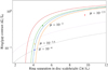Fig. 11. Contrast between rigs and gaps versus radial separation. The plain curves are estimated from the theory (Eq. (19)) while the diamond markers are points measured from simulations. The blue, orange, green, and red colours correspond respectively to μeq = 10−4,  10−3.5,  10−3, and 10−2.5. Dotted lines delimit the region above which dust can be concentrated within the rings, assuming H/R = 0.05 (black) and H/R = 0.1 (purple). See Sect. 4.7 for further detail.

4.6. Ring separation

So far, we have simply measured the ring separation as the most prominent k_x in simulations, but we also want to know if it is possible to predict this quantity from the linear theory. For large magnetisation (μ_eq = 10⁻² and 10^−2.5), this corresponds roughly to the radial scale that maximises the theoretical growth rate. However, for smaller magnetisation, this is no more the case. For instance, the prominent modes in simulation with μ_eq = 10⁻⁴ corresponds to k_x = 5k_x0 = 1.5 H⁻¹ and 6k_x0 = 1.8 H⁻¹, while the linear theory gives a maximum growth rate at k_x ≃ 0.45 H⁻¹. Actually, this is not in contradiction with the theory since σ appears to be quite flat with k_x in this regime. The reason is that turbulent dissipation is low (Pm_t = 25) and permits small scales axisymmetric modes to be amplified with significant growth rates. Modes then compete with each other and it becomes extremely difficult to predict the spacing from linear theory. The initial amplitude will be probably a decisive factor in the selection of the dominant mode(s). Such amplitude depends on the spectrum of the initial turbulence phase, which is a priori difficult to predict. We find (not shown here) that the spectrum of B_z associated with the initial turbulence peaks around k_x = 6k_x0 and beyond for μ_eq = 10⁻⁴, while it peaks at much lower k_x ≲ 0.3 in the case μ_eq = 10⁻². For μ_eq = 10⁻⁴, there is a difference of roughly a factor of 25 in initial energy between the k_x = 6k_x0 mode and the large-scale mode which, in principles, should grow fastest (k_x ≃ 0.45 H⁻¹). Therefore, it is likely that the ring spacing in our simulations is partly ruled by the initial turbulent conditions. Whether the spectrum of this turbulence is universal or depends on the historic and detailed physics of the disc remains an open question. We note however that all simulations, even in 3D (see Sect. 5), indicate a similar trend that the ring spacing increases with magnetisation. We finally emphasise that it does not depend too much on horizontal box size (see a comparison with small box Riols & Lesur 2018) or resolution.

4.7. Criterion for dust concentration

With the result of Sect. 4.5, we can infer a minimum magnetisation μ for which dust can accumulate into the gaps. A simple criterion is that the local pressure gradient in the disc have to be positive:

$$\begin{array}{c}\hfill {\displaystyle \frac{1}{P_0}}\left({\displaystyle \frac{\partial P}{\partial R}}\right)={\displaystyle \frac{1}{P_0}}\left({\displaystyle \frac{\partial P_0}{\partial R}}\right)+k_{\mathrm{R}}{\displaystyle \frac{\mathrm{\Delta }\mathrm{\Sigma }}{{\mathrm{\Sigma }}_0}}>0,\end{array}$$(20)

where P₀ is the mean equilibrium pressure profile and k_R the local radial wave number of the ring perturbation. A typical disc model, which matches disc observations (Andrews et al. 2009), has

$$\begin{array}{c}\hfill P_0\propto R^{-11/4}\text{and then}{\displaystyle \frac{1}{P_0}}\left({\displaystyle \frac{\partial P_0}{\partial R}}\right)=-{\displaystyle \frac{11}{4R}}.\end{array}$$(21)

The criterion for dust accumulation becomes:

$$\begin{array}{c}\hfill \left({\displaystyle \frac{\mathrm{\Delta }\mathrm{\Sigma }}{{\mathrm{\Sigma }}_0}}\right)\gtrsim {\displaystyle \frac{11}{4}}\left({\displaystyle \frac{H}{R}}\right)\frac{1}{k_{\mathrm{R}}H}·\end{array}$$(22)

The black and purple dotted lines in Fig. 11 delimit the region above which a radial concentration of dust is possible, respectively for H/R = 0.05 and H/R = 0.1. We predict that magnetisations greater than 10⁻⁴ or 10^−3.5 will lead to the formation of dusty rings. A more accurate estimation would require to take into account the radial diffusion of particles by the turbulence, which depends on the grain size and the nature of non-ideal effects, but this is beyond the scope of this paper.

5. 3D simulations

We extended our analysis to 3D simulations and show that ring structures exhibit properties that are again compatible with the instability model of Sect. 3.

5.1. Dependence on diffusive processes

First, we performed three different simulations for μ_eq = 10⁻³, respectively with no explicit diffusion, ohmic resistivity η = 0.01 and ambipolar diffusion Am_mid = 1. These simulations are initialised with random perturbations and are computed with L_x = L_y = 20 H, L_z = 8 H and resolution N_X = N_Y = 256, N_Z = 128. The top panels of Fig. 12 show that in all cases, zonal flows are produced, with growth rates and size that can substantially vary from on case to another. To help the analysis, we show in the lower panels the evolution of the mean transport coefficients α_ν, α_L, and mean mass loss efficiency ζ. In the ideal limit (simulation without explicit diffusion), these quantities are almost identical to those obtained in 2D (see Fig. 6 for comparison). However, the ring structure is much wider and takes longer time to form. The growth rate, measured from the left panel of Fig. 13 is indeed σ_3D ≃ 0.0034 ≃ σ_2D/2.5. The main difference is that the turbulent magnetic diffusivity η_t in 3D is considerably enhanced by the azimuthal (or non-axisymmetric) MRI dynamics. We indeed measure η ≃ 0.12 which corresponds to $P{m}_{\mathrm{t}}^{3\mathrm{D}}\simeq 2\ll P{m}_{\mathrm{t}}^{2\mathrm{D}}$, in agreement with other 3D numeric simulations (Lesur & Longaretti 2009). Therefore, according to the linear theory, the growth rate is reduced and drops rapidly with k_x (unlike the 2D case for which it was quite flat.) The maximum growth rate σ ≃ 0.0039 is obtained for k_xH = 0.2 and stability is reached for k_xH ≳ 0.42. This explains why we obtain a single ring in the 3D case, while three or four rings were obtained in 2D. We note that, unlike the 2D case, α does not drop significantly after saturation of the instability and vigorous turbulent motions persist along with the zonal structure.

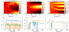Fig. 12. Top: space-time diagram showing the column density as a function of time and x, in 3D turbulent simulations with μeq = 10−3. Left panel: no explicit diffusion; centre panel: ohmic diffusion (Rm = ΩH2/η = 100); right panel: ambipolar diffusion (Ammid = 1). The density is integrated within z ± 1.5H. Bottom panels: for each run, time-evolution of turbulent αν, laminar αL and ζ the mass loss efficiency.

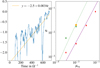Fig. 13. Left: time-evolution of ${\widehat{b}}_z$, the normalised projection of Bz onto the prominent axisymmetric Fourier mode (kx = 2π/Lx) in the ideal simulation with μeq = 10−3. Right: growth rate of the linear instability as a function of the magnetisation μ. The red diamond markers are measures from 3D ideal simulations. The green and yellow crosses are those measured in resistive and ambipolar runs. The plain lines correspond to model predictions, using similar scaling relations as (17), but with ηt = 0.5αν in the ideal case.

In non-ideal simulations, Fig. 12 (bottom panels) indicates that the wind mass loss efficiency ζ ≃ 0.015 is comparable to that in the ideal case. However, the turbulent stress is weak or even reduced to zero in the ambipolar case. The radial transport of angular momentum is provided essentially by the laminar component of the stress −⟨B_x⟩⟨B_y⟩. Azimuthal structures are very faint and have little impact on the unstable dynamics. We did indeed check that turbulent diffusion of B_z structures is negligible compared to the explicit one. As a consequence, growth rates are much larger than in the ideal case. We measure respectively σ = 0.018 and σ = 0.021 in the ohmic and ambipolar simulations. Using an extension of the linear theory (see Appendix B) in the limit α_L ≫ α_ν, we find that the theoretical growth rates match with the numerical values.

We note that σ is twice as big as the 2D axisymmetric case. We attribute this difference to the fact that ζ is on average twice as large as in 2D. Finally, with ambipolar diffusion, the number of rings is identical between the 2D and 3D case. With pure ohmic diffusion, the 3D simulation exhibits a single ring (instead of 3 in 2D). It is possible that the stronger laminar stress in 3D (a factor ≳2) favours the emergence of larger scale structures, thought initial conditions may also play a secondary role in the final shape.

5.2. Dependence on magnetisation μ

Finally, we ran a set of 3D ideal simulations (without explicit diffusion) by varying μ. We scanned a large range of magnetisations from μ_eq = 10⁻⁴ to 10⁻¹. For the largest magnetisations ( μ = 10⁻² and 0.08), we used a box of size L_x = 30 and 40 H respectively. Two or three rings are obtained for μ = 10⁻⁴ while a single ring is obtained for intermediate magnetisations. In the extreme case (μ ∼ 0.08), three or four rings form at the very early phase, but rapidly merge into a single ring. The growth rates of each prominent modes are shown in the right panel of Fig. 13 (red diamonds). We superimposed the theoretical growth rate σ(μ) (purple line) obtained by using the linear theory of Sect. 3. Here we assumed the same scaling relations for α and ζ as in 2D (Eq. (17)) but with η_t = 0.5α_ν. The theory reproduces quite well the numerical values, except maybe in the large magnetisation regime (μ ∼ 0.08). In the same figure, we also plot the numerical growth rates obtained in the resistive run (yellow marker) and those measured in ambipolar runs (green markers). The green dashed line accounts for the growth rate computed with an extension of the linear theory, in the regime α_L ≫ α_ν (see Appendix B) assuming ζ = 7 μ^0.85 and α_ν = 0; α_L = 4μ^0.45.

6. Discussion and conclusion

In summary, we showed that the ring and gap structures obtained in simulations of magnetised discs are formed via a linear instability. The process is generic and works in all geometrical configurations (2D or 3D), with or without turbulence, and in various diffusive regimes (ideal, ohmic or ambipolar). This instability is driven by a magnetic wind, associated with a large-scale poloidal field, and relies on the assumption that the mass loss rate increases locally with the magnetisation. The process works as follows:

• A small radial perturbation of density generates a radial flow directed towards the gaps, via the turbulent stress if α ≠ 0.

• The magnetic field, initially uniform, is radially transported towards the gaps.

• The excess of poloidal flux induces a stronger wind and an excess of ejected mass in the gaps.

• The initial density perturbation is thus reinforced.

We showed that in theory, the instability exists in the “no-stress” regime (α = 0). In that case, the radial flow results simply from angular momentum conservation. Indeed, assuming a geostrophic balance and an initial density perturbation, an azimuthal or zonal flow is produced. Therefore, the inertial term in the azimuthal direction produces a radial flow opposed to the initial density ring. However in practice the radial transport of matter and magnetic field is mainly (or even totally) induced by the viscous stress. Growth rates are typically of the order of the mass loss rate efficiency ζ = (ρu_z)_∣z = H/(ΣΩ⁻¹). In Sects. 4 and 5, we brought several evidence that such linear instability is at work in our MHD simulations. We showed in particular that axisymmetric modes undergo exponential growth in the early phase of the simulations, at rates compatible with the linear theory. A remarkable result is that growth rates increase rapidly with μ, and can be of order ≃0.1 Ω for μ = 0.1. This is a direct consequence of the wind reinforcement at large μ. Although the instability can theoretically exist in the limit of small wavenumbers, the rings separation is set by non-ideal processes in the disc and is typically ≃10 H for realistic diffusion coefficients. The final ring density contrast can be also estimated from a simple saturation predictor. Our model suggests that in typical T-Tauri discs with Σ ∝ R⁻¹, the dust accumulates into the gas rings for magnetisation μ ≳ 10⁻⁴. We finally provided detailed diagnostics of the axisymmetric flow, which are all consistent with the instability mechanism described above.

Unlike the mechanism suggested by Lubow et al. (1994) and Cao & Spruit (2002), the magnetic torque exerted by the wind is unnecessary here. We note that our linear analysis has been carried out around antisymmetric equilibria, for which the mean vertical stress and accretion flow are zero. Given its robustness, we think that the inclusion of a mean wind torque in our model will not dramatically affect the process, though an extension of the linear theory needs to be developed in this configuration. One possible effect is that the ring structures will be advected by the mean accretion flow and therefore slowly drift towards the central object. Global simulations with ambipolar diffusion have shown that ring structures persist despite the recurrent change in the large-scale wind geometry and vertical symmetries during the disc evolution (Béthune et al. 2017; Suriano et al. 2019). Further investigations will nevertheless be necessary to characterise the instability mechanism in the global configuration. Another caveat is related to the effect of boundary conditions and mass replenishment. Indeed, the mass loss rate is known to depend on the location of the vertical boundary (Fromang et al. 2013), as the outflow never crosses the fast magnetosonic point. The growth rate is then impacted too, according to our calculations. We then expect that the dependence of growth rates on μ is still correct, but that the absolute values of σ might depend on the external environment of the disc, but also on the topology of magnetic fields and wind launching conditions, which in reality can differ from the simulations and from object to objects. Regarding the mass replenishment procedure, it takes place on a long timescale, similar to the instability timescale. However, we think that this does not affect the whole process since it is independent on the radial coordinate. We also conducted simulations without replenishment and found that rings still form within the same timescale, despite the progressive loss of mass experienced by the disc. This indicates that mass replenishment does not play any role in the ring formation mechanism.

We think that the process described in this paper could have important implications for discs around young stars. Observationally, there are indications that some discs may emit a wind through the action of a large scale poloidal field. Indeed recent studies have reported low-velocity molecular outflow consistent with MHD winds in Class 0 and I discs (Launhardt et al. 2009; Bjerkeli et al. 2016; Tabone et al. 2017; Hirota et al. 2017; Louvet et al. 2018), although alternative processes are not excluded (photo-evaporation winds or jet “cocoon”). In theory, the magnetic flux from the parental core during the disc formation could be sufficient to provide the degree of disc magnetisation required for the launching of a wind. However an important unknown is how the poloidal magnetic flux is radially transported during the disc lifetime. If such transport is efficient, as is suggested by recent works (Guilet & Ogilvie 2013; Zhu & Stone 2018), the wind instability process described in this paper may be possible during the early stages of the disc evolution (Class 0 to Class II). As shown in Sect. 4, the instability form long-lived rings of size ≫H, which might remain stable during a large fraction of the disc lifetime. Such wind-driven instability could potentially explain the gaps imaged by ALMA or SPHERE in young discs like HL Tau or eventually leads to cavities like those observed in transitional discs (an alternative is the transonic wind-driven accretion recently proposed by Wang & Goodman 2017).

Recent MHD simulations with similar setup (Riols & Lesur 2018) have shown that the pressure maxima associated with the rings can efficiently trap dust grains of intermediate size (mm to dm). This could be directly relevant for planet formation theory, as it may help to overcome the “radial-drift” barrier (growth of grains to pebbles) and the “fragmentation” barrier (growth from planetesimals to planets) during the early phases when dust abounds (Birnstiel et al. 2016). Indeed, the confinement of solids in pressure maxima can stop the radial migration of grains, accelerate their growth, and prevent their fragmentation (Gonzalez et al. 2017). Further work is needed to understand how fast grain can grow and how the dust back-react on the gas rings. Another interesting avenue of research is to investigate the interaction between these rings and the disc gravitational instability, which is expected in class 0 and class I discs (Tobin et al. 2013; Mann et al. 2015). It is indeed unclear whether self-gravity could enhance or destroy the zonal MHD flows.

Finally, the linear instability identified in this paper could be applied to other accreting systems, such as active galactic nuclei, dwarf novae or X-ray binaries. Indeed some of these objects show signatures of strong jets, potentially driven by large scale poloidal fields via a magnetocentrifugal effect. The spontaneous formation of rings via a linear instability could have important consequences in their dynamics and their variability.

Acknowledgments

This work acknowledges funding from The French ANR under contracts ANR-17-ERC2-0007 (MHDiscs). This work was granted access to the HPC resources of IDRIS under the allocation A0040402231 made by GENCI (Grand Equipment National de Calcul Intensif). Part of this work was performed using the Froggy platform of the CIMENT infrastructure (https://ciment.ujf-grenoble.fr), which is supported by the Rhône-Alpes region (GRANT CPER07-13 CIRA), the OSUG@2020 labex (reference ANR10 LABX56) and the Equip@Meso project (reference ANR-10-EQPX-29-01) of the programme Investissements d’Avenir supervised by the Agence Nationale pour la Recherche.

References

Appendix A: Linearisation of total stress in the azimuthal momentum equation

In this appendix, we describe how we linearised the total stress in the y-momentum equation (radial plus vertical) around a given disc equilibrium. For that we used assumptions (2) and (3) of Sect. 3.6. These assumptions are checked numerically for unstable modes around a laminar disc equilibrium (see Appendix C). Using the formalism of Sect. 3 and Eqs. (7) and (8), the linearised quantities are

$$\begin{array}{c}\hfill \mathrm{\Sigma }{\overline{T}}_{\mathit{yx}}={\mathrm{\Sigma }}_0{\alpha }_{{\nu }_0}(\widehat{\mathrm{\Sigma }}+q\widehat{\mu })c_{\mathrm{s}}^2-B_{x_0}\underline{B_{y_0}}{\widehat{b}}_y-B_{y_0}\underline{B_{x_0}}{\widehat{b}}_x\end{array}$$(A.1)

$$\begin{array}{c}\hfill W_{\mathit{yz}}=-\underline{B_{y_0}}{B}_{z_0}({[{\widehat{b}}_z]}_{-}^{+}+{[\delta {\widehat{b}}_y]}_{-}^{+}).\end{array}$$(A.2)

Using the solenoidal condition, integrated azimuthally and vertically, we obtain that $B_{z_0}{[{\widehat{b}}_z]}_{-}^{+}=-i{k}_x\underline{B_{x_0}}{\widehat{b}}_x$. Therefore, the term associated with the vertical stress perturbation compensates exactly the term $-B_{{\mathit{y}}_0}\underline{B_{x_0}}{\widehat{b}}_x$ in the laminar radial stress. Adding W_yz and the x derivative of the averaged radial stress gives:

$$\begin{array}{cc}\hfill {\displaystyle \frac{\partial }{\partial x}}\left(\mathrm{\Sigma }{\overline{T}}_{\mathit{yx}}\right)+W_{\mathit{yz}}& =i{k}_x{\mathrm{\Sigma }}_0{c}_{\mathrm{s}}^2[{\alpha }_{{\nu }_0}(\widehat{\mathrm{\Sigma }}+q\widehat{\mu })+{\alpha }_{{\mathrm{L}}_0}{\widehat{b}}_y]\hfill \\ \hfill & -i{k}_x{B}_{z_0}\underline{B_{y_0}}{[{\widehat{b}}_y]}_{-}^{+}\hfill \end{array}$$(A.3)

with ${\alpha }_{{\mathrm{L}}_0}=-\underline{B_{x_0}}{B}_{{\mathit{y}}_0}/({\mathrm{\Sigma }}_0{c}_{\mathrm{s}}^2)$. We needed then to relate the perturbation ${\widehat{b}}_{\mathit{y}}$ to the variables of the reduced model $\widehat{\mathrm{\Sigma }},\widehat{\mu }$ or û. For that, we assumed that vertically, the disc is in a magneto-hydrostatic equilibrium and the magnetic field is essentially toroidal:

$$\begin{array}{c}\hfill {\displaystyle \frac{\partial }{\partial z}}(\rho c_{\mathrm{s}}^2+{\displaystyle \frac{B_y^2}{2}})=-\rho z{\mathrm{\Omega }}^2.\end{array}$$(A.4)

This is true below the Alfven point, where inertial terms of the wind are small compared to magnetic pressure. If we integrate Eq. (A.4) between −z_d and z_d, we obtain immediately that any perturbation of B_y is symmetric with respect to the midplane ${[{\widehat{b}}_{\mathit{y}}]}_{-}^{+}=0$ (if the background equilibrium B_y is also symmetric). We then integrated Eq. (A.4) between z_i and z, with z_i chosen to have $B_{\mathit{y}}^2[z_i]=⟨\underline{\delta B_{\mathit{y}}^2}⟩$. This altitude is always defined since B_y is a decreasing function of z and is located in general below the Alfven point since B_y is close to 0 at this altitude. By averaging in z and assuming ρ[z_i]≈0, we obtain

$$\begin{array}{c}\hfill ⟨\rho c_{\mathrm{s}}^2⟩+{\displaystyle \frac{⟨B_y⟩{⟨B_y⟩}^{\ast }}{2}}=\langle {\displaystyle {\int }_{z_i}^z-\rho (z\prime )z\prime {\mathrm{\Omega }}^2}\mathrm{d}z\rangle .\end{array}$$(A.5)

If we assume that the density profile is not too far from a Gaussian distribution of width H_m = hH with h >  1, then we have:

$$\begin{array}{c}\hfill {\displaystyle {\int }_{z_i}^z\rho (z\prime )z\prime {\mathrm{\Omega }}^2}\mathrm{d}z\prime \simeq -\rho h^2{c}_{\mathrm{s}}^2\end{array}$$(A.6)

and we find

$$\begin{array}{c}\hfill ⟨B_y⟩⟨\underline{B_y}⟩\simeq 2(h^2-1)\mathrm{\Sigma }{c}_{\mathrm{s}}^2.\end{array}$$(A.7)

We linearised this relation and obtain the following relation for the dimensionless toroidal perturbation

$$\begin{array}{c}\hfill {\widehat{b}}_y\simeq \lambda \widehat{\mathrm{\Sigma }}\text{with}\lambda ={\displaystyle \frac{1}{2}}{\displaystyle \frac{h^2-1}{{\mu }_{y_0}}}\simeq 0.5\end{array}$$(A.8)

${\mu }_{0_y}=B_{y_0}^2/(2\Sigma c_{\text{s}}^2)$ is the “toroidal magnetisation”. The total linearised stress can be then written

$$\begin{array}{c}\hfill {\displaystyle \frac{\partial }{\partial x}}\left(\mathrm{\Sigma }{\overline{T}}_{\mathit{yx}}\right)+W_{\mathit{yz}}=i{k}_x[({\alpha }_{{\nu }_0}+\lambda {\alpha }_{{\mathrm{L}}_0})\widehat{\mathrm{\Sigma }}+{\alpha }_{{\nu }_0}q\widehat{\mu }]{\mathrm{\Sigma }}_0{c}_{\mathrm{s}}^2.\end{array}$$(A.9)

Appendix B: Extension of the linear theory to laminar discs or discs with strong toroidal field

In this appendix, we have relaxed assumptions (1) and (3) in Section 3.6 and extended the linear analysis to a more general configuration. The geostrophic balance is replaced by a magneto-geostrophic balance, into which we included the effect of toroidal magnetic pressure. The radial stress can be purely laminar or a mix of both turbulent and laminar components. The following calculation applies in particular to discs with ambipolar diffusion. The linearised system of equations is:

$$\begin{array}{c}\hfill \left(\begin{array}{ccc}\sigma +{\zeta }_0& i{k}_x& p{\zeta }_0\\ {\displaystyle \frac{\sigma }{2}}(1+{\mu }_{y_0}\lambda )+{\alpha }_{{\nu }_0}+\lambda {\alpha }_{{\mathrm{L}}_0}& -{\displaystyle \frac{i}{2k_x}}& {\alpha }_{{\nu }_0}q\\ \sigma +{\eta }^{\star }{k}_x^2& 2i{k}_x& \sigma +{\eta }^{\star }{k}_x^2\end{array}\right)\left(\begin{array}{c}\widehat{\mathrm{\Sigma }}\\ \widehat{u}\\ {\widehat{b}}_z\end{array}\right)=0\end{array}$$(B.1)

with λ ≈ 0.5, a parameter introduced in Appendix A and ${\mu }_{0_y}=B_{y_0}^2/(2\Sigma c_{\text{s}}^2)$ the toroidal magnetisation of the equilibrium. The growth rates follow the dispersion relation

$$\begin{array}{c}\hfill A{\sigma }^2+B\sigma +C=0\end{array}$$(B.2)

with

$$\begin{array}{cc}\hfill A& =1+k_x^2(1+{\mu }_{y_0}\lambda )\hfill \\ \hfill B& =2k_x^2[{\alpha }_{{\nu }_0}(1+q)+\lambda {\alpha }_{L_0}]-{\zeta }_0[p-1+2p{k}_x^2(1+{\mu }_{y_0}\lambda )]\hfill \\ \hfill & +{\eta }^{\star }[k_x^2+k_x^4(1+{\mu }_{y_0}\lambda )]\hfill \\ \hfill C& =-4{\zeta }_0{k}_x^2[{\alpha }_{{\nu }_0}(p-q)+p\lambda {\alpha }_{{\mathrm{L}}_0}]\hfill \\ \hfill & +{\eta }^{\star }{k}_x^2[{\zeta }_0(1-p)+2{\alpha }_{{\nu }_0}(1-q)k_x^2+2\lambda {\alpha }_{{\mathrm{L}}_0}{k}_x^2].\hfill \end{array}$$(B.3)

We note that the case with a pure laminar stress is equivalent to that of a pure turbulent stress, but with q = 0. Thus, the instability criterion for laminar disc is less restrictive. In practise, given the fact that q = 0 and that turbulent diffusion is absent, growth rates can be enhanced (by a factor ≈2) compared to the turbulent case. A strong toroidal field can also help the instability, by affecting the geostrophic equilibrium and enhancing the zonal flows.

Appendix C: Stability of laminar disc with initial 1D uniform wind

To rigorously demonstrate the existence of an instability, similar to that predicted in Sect. 3, we use a very simple setup which consists of an initial uniform and laminar wind solution (independent on x). In that case, the radial stress is provided by the mean −B_xB_y relative to the laminar solution.

The first step is to compute a wind equilibrium in the local frame. For that, we employ the same technique as Lesur et al. (2013): we run a 1D shearing box simulation with an initial hydrostatic disc threaded by a vertical field of strength B_z0 = 0.044 (μ_eq = 10⁻³). We added some random noise at t = 0 and let the system evolves until it reaches a new equilibrium. In-between, an MRI mode is triggered and lead to the launch of a magneto-centrifugal wind. Figure C.1 (top) shows the equilibrium obtained in a box that spans −15 to 15H in the vertical direction. This class of solution is characterised by a very strong toroidal field and develops only if the system is initialised with a very clean 1D perturbation, so it is likely that it is never encountered in nature. The wind is however more realistic with mass loss efficiency ζ₀ ≃ 0.01.

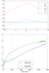Fig. C.1. Top: some quantities related to the 1D wind equilibrium. Bottom: amplitude (in logarithm) of the unstable Fourier mode kx = π/10 as a function of time. The background equilibrium is a laminar 1D wind computed for μeq = 10−3. Blue and green lines are, respectively, the surface density and vertical magnetic field perturbation. The blue dashed lines delimits the linear growth phase.

We then ran a 2D axisymmetric simulation, starting from the wind solution and add a small perturbation of the form exp(ik_xx) with k_x = 2π/L_x. Here we use a box size L_x = 20H and resolution (N_X, N_Z)=(256, 512). Figure C.1 (bottom) shows the time-evolution of the axisymetric perturbation ${\widehat{b}}_z$ and $\widehat{\mathrm{\Sigma }}$, projected onto the Fourier component k_x = 2π/L_x. Clearly, the mode is amplified exponentially during the first 200 Ω⁻¹ with growth rate σ ≃ 0.0074. We show in Fig. C.2 the shape of the unstable mode in the poloidal (x,z) plane. The density field develops a ring structure while the magnetic perturbation, anti-correlated with ρ, forms an inclined shell similar to that obtained in 3D turbulent simulations (see Fig. 2 for comparison). The radial velocity of the mode is anti-correlated with ${\widehat{\mathit{v}}}_{\mathit{y}}$ and directed towards the gap. The outflow and mass loss rate perturbations ρ₀û_z are positive inside the gap and negative outside. All of these properties are indications that the mode is triggered by the same instability as described in Sect. 3. One other interesting result is the apparent correlation between the density and the B_y structures, near the midplane. Such behaviour results from the magneto-hydrostatic equilibrium in the vertical direction (very well checked) and actually confirms our calculation in Appendix A. In particular we find $\lambda ={\widehat{b}}_{\mathit{y}}/\widehat{\mathrm{\Sigma }}\simeq 0.2$ when quantities are integrated vertically up to the Alfven point (instead of λ ≃ 0.5 in Appendix A). This parameter does not seem to depend on the integration boundary neither on k_x.

We finally achieved the same simulation for different k_x. The growth rates obtained for seven different radial wavenumbers are shown in Fig. C.3 (red diamond markers). The blue dashed curve is the model prediction, assuming α_L = 0.4, ζ₀ = 0.01, λ ≃ 0.2, λμ_0y = 3.2 and p = 0.5. We note that we use the extended model of Appendix B to compute the growth rates. The value of p is different from turbulent simulations and has been obtained by varying the magnetisation and measuring ζ of different 1D wind solutions. Although the maximum growth rate is in agreement with the numerical data, the behaviour at large k_x is not well reproduced by our model. The reason is the omission of the EMF term u_zb_x in the induction equation, which clearly enhances the instability at large k_x. We measured the ratio u_zb_x/u_xb_z for each k_x and include in the model a correction factor c_o(k_x) in the linearised induction equation. With such a correction, we obtain a very good match between the numerical and theoretical growth rates at large k_x (plain green curve in Fig. C.3).

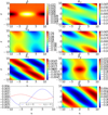Fig. C.2. Shape, in the poloidal plane, of the unstable axisymmetric mode kx = π/10 around the 1D wind equilibrium (μeq = 10−3).

Fig. C.3. Growth rate of axismmyetric modes measured in the laminar-wind simulations for different kx (red diamond makers). The blue-dashed curve shows the theoretical growth rate predicted from the model extension in Appendix B (assuming a pure laminar stress). The green plain curve shows the same model but taking into account the uzBx term in the induction equation (this term is simply estimated by calculating the ratio uzBx/uxBz associated with the unstable mode in simulations.

Appendix D: Check of model assumptions in simulations

To check the assumptions made in Sect. 3.6 and validate the linear theory of Sect. 3, we examine in details the mass, momentum, and magnetic budget in the 2D ambipolar run with μ = 10⁻³. Figure D.1 shows the different flux and source terms in Eqs. (3)–(6), averaged during the growth phase (delimited by the dashed lines in Fig. D.2). The terms are calculated in real space (and thus comprise all the axisymmetric modes) and are integrated within ±1H. The first panel shows that the gaps are depleted by the vertical mass flux ${\dot{\sigma }}_{\mathit{w}}$ while they are re-filled by the radial mass flux. It can be noted that the first term is slightly larger than the second. This ensures that the instability is driven by the outflow. The second panel clearly demonstrates that perturbations are in a geostrophic balance (Assumption 1 in Sect. 3.6), the Coriolis force being equilibrated by the radial thermal pressure gradient. In the azimuthal direction (third panel), both the radial flux of turbulent stress and the inertial term $\sim \sigma {\mathrm{\Sigma }}_0{\overline{\mathit{v}}}_{\mathit{y}}$ contribute to the production of v_x, directed towards the gaps. As suggested by the linear equations in Sect. 3.6, the inertial term due to the zonal flow can be an additional source of radial transport and even substitute for the α viscosity.

In the final panel we show that the vertical field in the gaps is mainly produced via the EMF term associated with radial motion –v_xB_z, as expected from the theory. The role of the vertical EMF component v_zB_x is more ambiguous: it seems to reinforce B_z in the nascent gaps at x ≃ −8 H and x = 0 but has a negative effect in the central gap at x = −5. Actually, Fig. D.2 shows that this structure has already evolved into a non-linear regime, unlike the others. In any case, this EMF term can be comparable to −v_xB_z and thus, our assumption (4) in Sect. 3.6 is not necessarily satisfied. The ambipolar term η_AJ_⊥y (with J_⊥y the y projection of the current perpendicular to B), is always negative within the gaps and positive outside. Therefore it tends to diffuse the magnetic field out of the gaps. This last result is clear evidence that the process forming rings (or gaps) is supported by the ideal terms and not by the ambipolar diffusion. In conclusion we showed that the force balance assumed in the linear regime (Sect. 3.6) is compatible with numerical data.

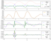Fig. D.1. Radial profiles of the flux and source terms in Eqs. (3)–(6), integrated vertically within z ± H and averaged in time during the linearphase for μeq = 10−3 and Am = 1. The linear phase is delimited by the vertical dashed lines in Fig. 9 (60 <  t <  200 Ω−1).

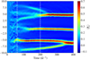Fig. D.2. Spacetime diagrams showing the vertically averaged Bz in the 2D ambipolar simulation (Ammid = 1, μeq = 10−3 and zd = 2H). The two vertical dashed lines delimit the “linear” phase, during which zonal modes, in Fourier space, grow exponentially.

All Figures

Fig. 1. Ring occurrence in MHD simulations with net vertical magnetic flux. The orange check mark means that zonal flow exist, but their persistence within the turbulent flow and their convergence with box size are uncertain at current time. (1) Suriano et al. (2017), (2) Bai & Stone (2014), (3) our own simulations, (4) Hawley (2001), (5) Kunz & Lesur (2013), (6) Béthune et al. (2016), (7) Krapp et al. (2018), (8) Bai (2015), (9) Riols & Lesur (2018), (10) Suriano et al. (2018, 2019).

In the text

Fig. 2. Example of a ring and gap structure and its surrounding outflow topology in the 3D shearing box simulation of Riols & Lesur (2018) with ambipolar diffusion. Top panel: gas density (colourmap in log scale) and streamlines (cyan lines) in the poloidal plane (x and z are respectively the radial and vertical coordinates). Bottom panel: vertical magnetic field (colourmap) and poloidal magnetic field lines (in white) showing the inclined “plume” structure from where most of the mass is extracted. The thickness of the lines is proportional to the field intensity.

In the text

	Fig. 3. Radial velocity computed from the 3D simulation of Fig. 2. It is averaged in the azimuthal direction, in z within ±1.5H and during the first 50 orbits (∼300 Ω−1), corresponding to the growth of the ring structure.
In the text

Fig. 4. Sketch illustrating the development of rings in accretion discs. The black and blue arrows represent the radial flow and the wind, respectively. The green patches correspond to density minima where the vertical field Bz and the magnetisation μ grow. In this representation, the poloidal field lines (// to the wind) do not bend in the midplane but cross the disc with some angle. This configuration is actually not intuitive but is encountered in various disc simulations around the midplane.

In the text

	Fig. 5. Growth rate of the wind-driven instability as a function of the radial wavenumber for different magnetic diffusivities. Parameters of the model have been chosen in agreement with numerical simulations for fiducial μeq = 10−3: αν ≃ 0.3, p ≃ 1, q ≃ 0.5, ζ0 ≃ 0.01.
In the text

	Fig. 6. Evolution of the transport coefficient αν, αL and the wind mass loss efficiency ζ in the 2D simulation without explicit diffusion (μeq = 10−3)
In the text

Fig. 7. Top: space-time diagram showing the column density as a function of time and x, in 2D axisymmetric turbulent simulations, for different magnetisation (left to right, μeq = 10−4,  10−3 and 10−2). The density is integrated within z ± 1.5H and runs were computed in the ideal limit (without explicit magnetic diffusion). Bottom panels: for each run, time-evolution of ${\widehat{b}}_z$, normalised projection of Bz onto the prominent axisymmetric Fourier mode (with largest amplitude). This mode corresponds respectively to kx = 6, 4 and 2kx0 for μeq = 10−4,  10−3 and 10−2, with kx0 = 2π/Lx the fundamental box radial wavenumber.

In the text

Fig. 8. Optimal growth rate of the instability as a function of the magnetisation μ. The red diamond markers are the growth rates of the most unstable Fourier mode measured in 2D ideal simulations. The orange and green crosses are those measured in resistive and ambipolar runs. The purple solid line correspond to the model prediction, using the scaling relations (17) and (18). The blue and yellow dashed lines use the same model but with constant η⋆ = 0.01 in both cases and constant αν = 0.1 for the last case.

In the text

	Fig. 9. Top panel: space-time diagrams showing the surface density Σ(x, t) in the 2D ambipolar simulation (Ammid = 1, μeq = 10−3 and zd = 2H). The two vertical dashed lines delimit the “linear” phase, during which zonal modes, in Fourier space, grow exponentially. Bottom panel: evolution of the Bz component projected onto the kx = 4kx0 mode.
In the text

	Fig. 10. Coefficients p and q measured from the 2D ideal simulation with μeq = 10−4. The red (respectively blue) line shows the ratio between the perturbation of ζ (respectively α) and the perturbation associated with magnetisation, as a function of time. Each quantity (ζ, α and μ) is projected onto the mode kx = 6kx0, averaged within z ± 2H and normalised to its mean.
In the text

Fig. 11. Contrast between rigs and gaps versus radial separation. The plain curves are estimated from the theory (Eq. (19)) while the diamond markers are points measured from simulations. The blue, orange, green, and red colours correspond respectively to μeq = 10−4,  10−3.5,  10−3, and 10−2.5. Dotted lines delimit the region above which dust can be concentrated within the rings, assuming H/R = 0.05 (black) and H/R = 0.1 (purple). See Sect. 4.7 for further detail.

In the text

Fig. 12. Top: space-time diagram showing the column density as a function of time and x, in 3D turbulent simulations with μeq = 10−3. Left panel: no explicit diffusion; centre panel: ohmic diffusion (Rm = ΩH2/η = 100); right panel: ambipolar diffusion (Ammid = 1). The density is integrated within z ± 1.5H. Bottom panels: for each run, time-evolution of turbulent αν, laminar αL and ζ the mass loss efficiency.

In the text

Fig. 13. Left: time-evolution of ${\widehat{b}}_z$, the normalised projection of Bz onto the prominent axisymmetric Fourier mode (kx = 2π/Lx) in the ideal simulation with μeq = 10−3. Right: growth rate of the linear instability as a function of the magnetisation μ. The red diamond markers are measures from 3D ideal simulations. The green and yellow crosses are those measured in resistive and ambipolar runs. The plain lines correspond to model predictions, using similar scaling relations as (17), but with ηt = 0.5αν in the ideal case.

In the text

	Fig. C.1. Top: some quantities related to the 1D wind equilibrium. Bottom: amplitude (in logarithm) of the unstable Fourier mode kx = π/10 as a function of time. The background equilibrium is a laminar 1D wind computed for μeq = 10−3. Blue and green lines are, respectively, the surface density and vertical magnetic field perturbation. The blue dashed lines delimits the linear growth phase.
In the text

	Fig. C.2. Shape, in the poloidal plane, of the unstable axisymmetric mode kx = π/10 around the 1D wind equilibrium (μeq = 10−3).
In the text

Fig. C.3. Growth rate of axismmyetric modes measured in the laminar-wind simulations for different kx (red diamond makers). The blue-dashed curve shows the theoretical growth rate predicted from the model extension in Appendix B (assuming a pure laminar stress). The green plain curve shows the same model but taking into account the uzBx term in the induction equation (this term is simply estimated by calculating the ratio uzBx/uxBz associated with the unstable mode in simulations.

In the text

	Fig. D.1. Radial profiles of the flux and source terms in Eqs. (3)–(6), integrated vertically within z ± H and averaged in time during the linearphase for μeq = 10−3 and Am = 1. The linear phase is delimited by the vertical dashed lines in Fig. 9 (60 <  t <  200 Ω−1).
In the text

	Fig. D.2. Spacetime diagrams showing the vertically averaged Bz in the 2D ambipolar simulation (Ammid = 1, μeq = 10−3 and zd = 2H). The two vertical dashed lines delimit the “linear” phase, during which zonal modes, in Fourier space, grow exponentially.
In the text

References

- ALMA Partnership (Brogan, C. L., et al.) 2015, ApJ, 808, L3 [NASA ADS] [CrossRef] [Google Scholar]
- Andrews, S. M., Wilner, D. J., Hughes, A. M., Qi, C., & Dullemond, C. P. 2009, ApJ, 700, 1502 [NASA ADS] [CrossRef] [Google Scholar]
- Andrews, S. M., Wilner, D. J., Zhu, Z., et al. 2016, ApJ, 820, L40 [NASA ADS] [CrossRef] [Google Scholar]
- Bai, X.-N. 2015, ApJ, 798, 84 [Google Scholar]
- Bai, X.-N. 2017, ApJ, 845, 75 [NASA ADS] [CrossRef] [Google Scholar]
- Bai, X.-N., & Stone, J. M. 2013, ApJ, 767, 30 [NASA ADS] [CrossRef] [Google Scholar]
- Bai, X.-N., & Stone, J. M. 2014, ApJ, 796, 31 [Google Scholar]
- Balbus, S. A., & Hawley, J. F. 1991, ApJ, 376, 214 [NASA ADS] [CrossRef] [Google Scholar]
- Baruteau, C., Crida, A., Paardekooper, S. J., et al. 2014, Protostars and Planets VI, 667 [Google Scholar]
- Béthune, W., Lesur, G., & Ferreira, J. 2016, A&A, 589, A87 [NASA ADS] [CrossRef] [EDP Sciences] [Google Scholar]
- Béthune, W., Lesur, G., & Ferreira, J. 2017, A&A, 600, A75 [NASA ADS] [CrossRef] [EDP Sciences] [Google Scholar]
- Birnstiel, T., Fang, M., & Johansen, A. 2016, Space Sci. Rev., 205, 41 [NASA ADS] [CrossRef] [Google Scholar]
- Bjerkeli, P., van der Wiel, M. H. D., Harsono, D., Ramsey, J. P., & Jørgensen, J. K. 2016, Nature, 540, 406 [NASA ADS] [CrossRef] [Google Scholar]
- Cao, X., & Spruit, H. C. 2002, A&A, 385, 289 [NASA ADS] [CrossRef] [EDP Sciences] [Google Scholar]
- Dipierro, G., Price, D., Laibe, G., et al. 2015, MNRAS, 453, L73 [NASA ADS] [CrossRef] [Google Scholar]
- Dong, R., Zhu, Z., & Whitney, B. 2015, ApJ, 809, 93 [NASA ADS] [CrossRef] [Google Scholar]
- Dullemond, C. P., & Penzlin, A. B. T. 2018, A&A, 609, A50 [NASA ADS] [CrossRef] [EDP Sciences] [Google Scholar]
- Flock, M., Ruge, J. P., Dzyurkevich, N., et al. 2015, A&A, 574, A68 [NASA ADS] [CrossRef] [EDP Sciences] [Google Scholar]
- Fromang, S., & Stone, J. M. 2009, A&A, 507, 19 [NASA ADS] [CrossRef] [EDP Sciences] [Google Scholar]
- Fromang, S., Latter, H., Lesur, G., & Ogilvie, G. I. 2013, A&A, 552, A71 [NASA ADS] [CrossRef] [EDP Sciences] [Google Scholar]
- Garufi, A., Benisty, M., Stolker, T., et al. 2017, The Messenger, 169, 32 [NASA ADS] [Google Scholar]
- Goldreich, P., & Lynden-Bell, D. 1965, MNRAS, 130, 125 [NASA ADS] [CrossRef] [Google Scholar]
- Gonzalez, J.-F., Laibe, G., & Maddison, S. T. 2017, MNRAS, 467, 1984 [NASA ADS] [Google Scholar]
- Gressel, O., Turner, N. J., Nelson, R. P., & McNally, C. P. 2015, ApJ, 801, 84 [NASA ADS] [CrossRef] [Google Scholar]
- Guan, X., & Gammie, C. F. 2009, ApJ, 697, 1901 [NASA ADS] [CrossRef] [Google Scholar]
- Guilet, J., & Ogilvie, G. I. 2013, MNRAS, 430, 822 [NASA ADS] [CrossRef] [Google Scholar]
- Hawley, J. F. 2001, ApJ, 554, 534 [NASA ADS] [CrossRef] [Google Scholar]
- Hawley, J. F., Gammie, C. F., & Balbus, S. A. 1995, ApJ, 440, 742 [NASA ADS] [CrossRef] [Google Scholar]
- Helled, R., & Bodenheimer, P. 2014, ApJ, 789, 69 [NASA ADS] [CrossRef] [Google Scholar]
- Hirota, T., Machida, M. N., Matsushita, Y., et al. 2017, Nat. Astron., 1, 0146 [Google Scholar]
- Isella, A., Guidi, G., Testi, L., et al. 2016, Phys. Rev. Lett., 117, 251101 [NASA ADS] [CrossRef] [Google Scholar]
- Johansen, A., Youdin, A., & Klahr, H. 2009, ApJ, 697, 1269 [NASA ADS] [CrossRef] [Google Scholar]
- Kley, W., & Nelson, R. P. 2012, ARA&A, 50, 211 [NASA ADS] [CrossRef] [Google Scholar]
- Konigl, A., & Wardle, M. 1996, MNRAS, 279, L61 [NASA ADS] [CrossRef] [Google Scholar]
- Krapp, L., Gressel, O., Benítez-Llambay, P., et al. 2018, ApJ, 865, 105 [NASA ADS] [CrossRef] [Google Scholar]
- Kunz, M. W., & Lesur, G. 2013, MNRAS, 434, 2295 [NASA ADS] [CrossRef] [Google Scholar]
- Launhardt, R., Pavlyuchenkov, Y., Gueth, F., et al. 2009, A&A, 494, 147 [NASA ADS] [CrossRef] [EDP Sciences] [Google Scholar]
- Lesur, G., & Longaretti, P.-Y. 2009, A&A, 504, 309 [NASA ADS] [CrossRef] [EDP Sciences] [Google Scholar]
- Lesur, G., Ferreira, J., & Ogilvie, G. I. 2013, A&A, 550, A61 [NASA ADS] [CrossRef] [EDP Sciences] [Google Scholar]
- Lesur, G., Kunz, M. W., & Fromang, S. 2014, A&A, 566, A56 [NASA ADS] [CrossRef] [EDP Sciences] [Google Scholar]
- Lightman, A. P., & Eardley, D. M. 1974, ApJ, 187, L1 [NASA ADS] [CrossRef] [Google Scholar]
- Louvet, F., Dougados, C., Cabrit, S., et al. 2018, A&A, 618, A120 [NASA ADS] [CrossRef] [EDP Sciences] [Google Scholar]
- Lubow, S. H., Papaloizou, J. C. B., & Pringle, J. E. 1994, MNRAS, 268, 1010 [NASA ADS] [CrossRef] [Google Scholar]
- Mann, R. K., Andrews, S. M., Eisner, J. A., et al. 2015, ApJ, 802, 77 [NASA ADS] [CrossRef] [Google Scholar]
- Mignone, A., Bodo, G., Massaglia, S., et al. 2007, ApJS, 170, 228 [Google Scholar]
- Moll, R. 2012, A&A, 548, A76 [NASA ADS] [CrossRef] [EDP Sciences] [Google Scholar]
- Okuzumi, S., Momose, M., Sirono, S.-I., Kobayashi, H., & Tanaka, H. 2016, ApJ, 821, 82 [NASA ADS] [CrossRef] [Google Scholar]
- Pinilla, P., Birnstiel, T., Ricci, L., et al. 2012, A&A, 538, A114 [NASA ADS] [CrossRef] [EDP Sciences] [Google Scholar]
- Riols, A., & Lesur, G. 2018, A&A, 617, A117 [NASA ADS] [CrossRef] [EDP Sciences] [Google Scholar]
- Riols, A., Ogilvie, G. I., Latter, H., & Ross, J. P. 2016, MNRAS, 463, 3096 [NASA ADS] [CrossRef] [Google Scholar]
- Salvesen, G., Armitage, P. J., Simon, J. B., & Begelman, M. C. 2016, MNRAS, 460, 3488 [NASA ADS] [CrossRef] [Google Scholar]
- Scepi, N., Lesur, G., Dubus, G., & Flock, M. 2018, A&A, 620, A49 [NASA ADS] [CrossRef] [EDP Sciences] [Google Scholar]
- Simon, J. B., & Armitage, P. J. 2014, ApJ, 784, 15 [NASA ADS] [CrossRef] [Google Scholar]
- Simon, J. B., Beckwith, K., & Armitage, P. J. 2012, MNRAS, 422, 2685 [NASA ADS] [CrossRef] [Google Scholar]
- Simon, J. B., Bai, X.-N., Armitage, P. J., Stone, J. M., & Beckwith, K. 2013, ApJ, 775, 73 [NASA ADS] [CrossRef] [Google Scholar]
- Steinacker, A., & Papaloizou, J. C. B. 2002, ApJ, 571, 413 [NASA ADS] [CrossRef] [Google Scholar]
- Suriano, S. S., Li, Z.-Y., Krasnopolsky, R., & Shang, H. 2017, MNRAS, 468, 3850 [NASA ADS] [CrossRef] [Google Scholar]
- Suriano, S. S., Li, Z.-Y., Krasnopolsky, R., & Shang, H. 2018, MNRAS, 477, 1239 [NASA ADS] [CrossRef] [Google Scholar]
- Suriano, S. S., Li, Z.-Y., Krasnopolsky, R., Suzuki, T. K., & Shang, H. 2019, MNRAS, 484, 107 [NASA ADS] [CrossRef] [Google Scholar]
- Suzuki, T. K., & Inutsuka, S.-I. 2009, ApJ, 691, L49 [NASA ADS] [CrossRef] [Google Scholar]
- Tabone, B., Cabrit, S., Bianchi, E., et al. 2017, A&A, 607, L6 [NASA ADS] [CrossRef] [EDP Sciences] [Google Scholar]
- Takahashi, S. Z., & Inutsuka, S.-I. 2014, ApJ, 794, 55 [NASA ADS] [CrossRef] [Google Scholar]
- Tobin, J. J., Chandler, C. J., Wilner, D. J., et al. 2013, ApJ, 779, 93 [NASA ADS] [CrossRef] [Google Scholar]
- Wang, L., & Goodman, J. J. 2017, ApJ, 835, 59 [NASA ADS] [CrossRef] [Google Scholar]
- Wünsch, R., Klahr, H., & Różyczka, M. 2005, MNRAS, 362, 361 [NASA ADS] [CrossRef] [Google Scholar]
- Zhu, Z., & Stone, J. M. 2018, ApJ, 857, 34 [NASA ADS] [CrossRef] [Google Scholar]