| Issue |
A&A
Volume 662, June 2022
|
|
|---|---|---|
| Article Number | A6 | |
| Number of page(s) | 13 | |
| Section | The Sun and the Heliosphere | |
| DOI | https://doi.org/10.1051/0004-6361/202142868 | |
| Published online | 26 May 2022 | |
Magnetic helicity and energy of emerging solar active regions and their erruptivity
1
Section of Astrogeophysics, Department of Physics, University of Ioannina, 45110 Ioannina, Greece
e-mail: This email address is being protected from spambots. You need JavaScript enabled to view it.
2
W. W. Hansen Experimental Physics Laboratory, Stanford University, Stanford, CA 94305-4085, USA
Received:
9
December
2021
Accepted:
4
February
2022
Abstract
Aims. We investigate the role of the accumulation of magnetic helicity and magnetic energy in the generation of coronal mass ejections (CMEs) from emerging solar active regions (ARs).
Methods. Using vector magnetic field data obtained by the Helioseismic and Magnetic Imager on board the Solar Dynamics Observatory, we calculated the magnetic helicity and magnetic energy injection rates as well as the resulting accumulated budgets in 52 emerging ARs from the start time of magnetic flux emergence until they reached a heliographic longitude of 45° West (W45).
Results. Seven of the ARs produced CMEs, but 45 did not. In a statistical sense, the eruptive ARs accumulate larger budgets of magnetic helicity and energy than the noneruptive ARs over intervals that start from the flux emergence start time and end (i) at the end of the flux emergence phase and (ii) when the AR produces its first CME or crosses W45, whichever occurs first. We found magnetic helicity and energy thresholds of 9 × 1041 Mx2 and 2 × 1032 erg. When these thresholds were crossed, ARs are likely to erupt. In terms of accumulated magnetic helicity and energy budgets, the segregation of the eruptive from the noneruptive ARs is violated in one case when an AR erupts early in its emergence phase and in six cases in which noneruptive ARs exhibit large magnetic helicity and energy budgets. Decay index calculations may indicate that these ARs did not erupt because the overlying magnetic field provided a stronger or more extended confinement than in eruptive ARs.
Conclusions. Our results indicate that emerging ARs tend to produce CMEs when they accumulate significant budgets of both magnetic helicity and energy. Any study of their eruptive potential should consider magnetic helicity together with magnetic energy.
Key words: Sun: magnetic fields / Sun: coronal mass ejections (CMEs) / Sun: photosphere / Sun: corona
© ESO 2022
1. Introduction
Solar active regions (ARs) are extended areas of the solar atmosphere (in the photosphere, their area ranges from 50 to 100 000 Mm2) with a magnetic field that is much stronger than that of their surroundings (see van Driel-Gesztelyi & Green 2015, and references therein). ARs are formed by the emergence of magnetic flux from the interior of the Sun. The first step in the formation of a simple bipolar AR is the emergence of an Ω-shaped flux tube; the intersections of the axial magnetic field of the tube with the photosphere causes the two magnetic polarities of the AR (see Schmieder et al. 2014; Archontis & Syntelis 2019, and references therein). During the emergence phase, the two main polarities move apart and small magnetic elements appear in between. Different bipoles in proximity may interact to form ARs with more complex configurations (e.g., Toriumi 2014).
Active regions are the source of explosive phenomena, the most violent of which are flares (i.e., sudden bursts of electromagnetic radiation) and coronal mass ejections (CMEs; i.e., large-scale expulsions of magnetized coronal plasma propagating through the heliosphere). These phenomena occur because both flux emergence (e.g., see Leka et al. 1996) and subsequent AR evolution may provide a large amount of free magnetic energy (i.e., the nonpotential part of the magnetic energy due to electric currents above the photosphere) that can be released via magnetic reconnection or some instability (e.g., see the review by Toriumi & Wang 2019).
Because the origin of flares and CMEs is magnetic, any attempt to study them requires an in-depth knowledge of the properties of the magnetic field. One of the key quantities that characterize magnetic fields is their magnetic helicity. It indicates how complex the field is by measuring the twist, writhe, and linkage of the field lines (e.g., see Pevtsov et al. 2014, and references therein). In ideal magnetohydrodynamics (MHD), magnetic helicity is a strictly conserved quantity (e.g., see Priest 2014), while in nonideal processes such as magnetic reconnection, it is conserved to an excellent approximation in plasmas with high magnetic Reynolds numbers (e.g., see Berger 1984; Pariat et al. 2015).
Several methods for estimating magnetic helicity have been developed (see Thalmann et al. 2021, for a comparison). They include (i) finite-volume methods (see Valori et al. 2016, for an extensive review and comparison of finite-volume methods), (ii) the connectivity-based method (Georgoulis et al. 2012), (iii) the twist number method (Guo et al. 2017), and (iv) helicity-flux integration methods (e.g., Chae 2001; Nindos & Zhang 2002; Pariat et al. 2005; Dalmasse et al. 2014, 2018). Methods (i) and (ii) provide the instantaneous magnetic helicity in a given volume, and the same is true for method (iii), with the exception that only the contribution of twist to the magnetic helicity is estimated. On the other hand, helicity flux integration methods provide only the helicity injection rate and hence the accumulated helicity during certain time intervals.
Although the role of free magnetic energy in the initiation of solar eruptions is well established (e.g., Schrijver 2009), the role of magnetic helicity is debated. Phillips et al. (2005) have suggested that helicity may not be at the heart of CME initiation processes. On the other hand, some authors (e.g., Low 1996) have conjectured that CMEs are the main agents through which the corona removes excess helicity. Similarly, Zhang et al. (2006, 2012) have suggested that an upper bound for the accumulation of magnetic helicity may exist, which, if exceeded, could create a nonequilibrium state leading to a CME. Furthermore, Kusano et al. (2003, 2004) proposed that the accumulation of a similar amount of positive and negative helicity can facilitate magnetic reconnection, leading to eruptive phenomena. Pariat et al. (2017) found that the ratio of the helicity of the current-carrying magnetic field to the total helicity represents a reliable eruptivity proxy, whereas both the magnetic energy and total helicity do not.
Observationally, the analysis of different data sets supports the important role of helicity in the initiation of eruptive events (see Pevtsov et al. 2014, for a review). For example, Nindos & Andrews (2004) fount that in a statistical sense, the coronal helicity resulting from the absolute values of the linear force-free field parameter is higher in ARs that produce major eruptive flares than in those that produce major confined flares. Similar conclusions were reached by LaBonte et al. (2007) and Park et al. (2008, 2010). Furthermore, Tziotziou et al. (2012) used the connectivity-based method developed by Georgoulis et al. (2012) and found a significant monotonic correlation between the instantaneous helicity and free magnetic energy of several ARs. They also found that the eruptive ARs were segregated from noneruptive ARs in both helicity and free magnetic energy, with helicity and free energy thresholds for the occurrence of major flares of 2 × 1042 Mx2 and 4 × 1031 erg, respectively. Nindos et al. (2012) showed that the initiation of major eruptions in a large emerging AR depended on the accumulation of both helicity and free magnetic energy and not on the temporal evolution of the variation of the background magnetic field with height. Some authors have reported (see Vemareddy 2017, 2019; Dhakal et al. 2020) that ARs that inject helicity with a predominant sign might be source regions of CMEs.
The association between the evolutionary stage of ARs and the occurrence of CMEs is complex. For example, Zhang et al. (2008) reported that the association with the emergence phase is only slightly higher than the association with the decay phase. Although decaying ARs are capable of producing eruptions, primarily due to magnetic flux cancellation, most of the eruptive activity often occurs from still emerging and evolving ARs and around the time at which their magnetic flux attains maximum values (Choudhary et al. 2013). The motivation of this study is to investigate the role of accumulation of both magnetic helicity and magnetic energy in the generation of CMEs from emerging ARs. Our study will demonstrate for the first time using the flux integration method that critical thresholds of magnetic energy and helicity exist above which an AR is expected with a fairly high probability to produce a CME. The next section describes our data base. Our method is given in Sect. 3, while the properties of the magnetic helicity and energy content of the ARs are presented in Sect. 4. In Sect. 5 we discuss the segregation of eruptive from noneruptive ARs in both magnetic helicity and energy. Our conclusions and a summary are presented in Sect. 6.
2. Data set
We compiled a catalog of emerging ARs that appeared on the solar disk during the ascending phase of solar cycle 24, from May 2010 to December 2012. The criteria we used to assemble our catalog were that (1) at the time of their emergence, the ARs should be located within 45° of the central meridian. (2) The ARs should emerge into relatively quiet photospheric areas without preexisting ARs. The first criterion was used to limit severe projection effects that may compromise magnetic field measurements at large central meridian distances. The selection of relatively quiet emergence sites aimed to minimize the contribution of preexisting strong magnetic fields to the budgets of the accumulated magnetic helicity and energy of the ARs. We further elaborate on this issue in Sect. 3.
For the implementation of the first criterion, we assembled a list of candidate emerging ARs by searching the solar AR reports compiled by the National Oceanic and Atmospheric Administration (NOAA) from 2010 to 20121. From the candidate ARs, we further selected those that emerged into the quiet Sun by visually inspecting monthly “quicklook” full-disk movies2 containing sketches of so-called HMI active region Patches (HARPs), which are coherent, enduring magnetic structures on the size scale of an AR. HARPs are identified in line-of-sight magnetograms obtained with the Helioseismic and Magnetic Imager (HMI; Scherrer et al. 2012; Schou et al. 2012) instrument on board the Solar Dynamics Observatory (SDO; Pesnell et al. 2012). Then we constructed time profiles of the unsigned magnetic flux of the resulting candidate ARs by using actual HMI magnetograms at a cadence of 12 h. We kept only those ARs whose time profiles of the flux rose monotonically for at least 18 hours above a low background (see also Schunker et al. 2016). For each AR, the flux emergence start time was assigned to the time beginning of that interval.
This procedure yielded a catalog of 52 emerging ARs. It is presented in Table 1. The two table entries where two NOAA AR numbers appear (labeled 11466+11468 and 11631+11632) correspond to cases in which the first major flux emergence episode was accompanied by a second episode nearby that also resulted in the formation of a NOAA AR. However, in each of these cases, EUV loops in AIA images reveal that the newly formed ARs are magnetically connected that justifies their treatment as single entities. In the second column of Table 1 we list the flux emergence start time (see above), which, in some cases, takes place before the time of the first recording of the AR by NOAA. The times when the ARs cross heliographic longitude of 45° West (hereafter referred to as W45) are given in the third column of Table 1.
Properties of emerging ARs.
For our study we employed HMI vector magnetic data (Hoeksema et al. 2014). In particular, we used the so-called HMI.SHARP_CEA_720s data series (Bobra et al. 2014), which contains Lambert cylindrical equal-area (CEA) projections of the photospheric magnetic field vector. For this HMI data product, the native vector field output from the inversion code was transformed into three spherical heliographic components, Br, Bθ, and Bϕ (Gary & Hagyard 1990), which relate to the heliographic field components as [Bx, By, Bz] = [Bϕ, −Bθ, Br] (see Sun 2013), where x, y, and z indicate the solar westward, northward, and vertical directions, respectively. The spatial resolution of the CEA vector field images is 0.03 CEA-degrees, which correspond to about 360 km per pixel at disk center. The cadence of our CEA datacubes was 12 min. For each AR, we calculated the magnetic helicity and energy injection rates from the time that the relevant Spaceweather HMI Active Region Patch (SHARP) data products become available to the W45 passage time of the AR.
For the detection of CMEs associated with our ARs, we used (1) movies of Large Angle and Spectrometric Coronagraph (LASCO) images that can be found in the LASCO CME Catalog3 (Gopalswamy et al. 2009) and (2) difference images from the Atmospheric Imaging Assembly (AIA, Lemen et al. 2012; Boerner et al. 2012) instrument on board SDO at 211 Å. This particular AIA channel was chosen because it shows better CME-related dimming regions, which were used (together with the appearance of ascending loops) as proxies for the determination of the CME sources. Seven of our 52 ARs produced a CME before W45° crossing (hereafter referred to as eruptive ARs) and 45 did not (hereafter referred to as noneruptive ARs; see Col. (8) of Table 1). The flares associated with each AR were obtained from the GOES catalog of X-ray flares4.
3. Method
For each AR of Table 1, we computed the rates of magnetic helicity and magnetic energy injection into the solar atmosphere. As was mentioned in Sect. 2, these quantities were computed from the time SHAPR data products became available for the ARs until the ARs reached a heliographic longitude of W45. In several cases the SHARP tracking algorithm starts tracking emerging ARs after their actual emergence, which results in lost data at the very beginning of the emergence. However, the missing data had a marginal effect on our results; in selected representative ARs, we retrieved the missing early emergence data from nominal full-disk vector magnetograms and found that the missing intervals contributed no more than than 0.1% to the total accumulated helicity and energy values derived by the SHARP data. Therefore, hereafter the time of the first available SHARP data products is referred to as flux emergence start time.
The expressions for the flux of magnetic helicity and magnetic energy across a surface S, like the photosphere, are
 (1)
(1)
 (2)
(2)
(see Berger 1984, 1999; Kusano et al. 2002), where AP is the vector potential of the potential field BP, Bt and Bn are the tangential and normal components of the magnetic field in the photosphere, and V⊥t and V⊥n are the tangential and normal components of the velocity V⊥, which is perpendicular to the field lines. The first terms of the right-hand side of Eqs. (1) and (2) give the magnetic helicity and energy flux, respectively, caused by the emergence of twisted field lines that cross the photosphere, while the second terms give the generation of helicity and energy flux, respectively, caused by the shearing and braiding of the magnetic field lines by the tangential motions on the solar surface.
The vector velocity field was derived by applying the differential affine velocity estimator for vector magnetograms (DAVE4VM; Schuck 2008) method to sequential coaligned pairs of the Bx, By, and Bz data cubes (see Sect. 2). The size of the apodization window we used was 19 pixels, as suggested by Schuck (2008). These velocities were corrected (e.g., see Liu & Schuck 2012; Liu et al. 2014) by removing the irrelevant contribution from the magnetic-field-aligned plasma flow using the formula
 (3)
(3)
where V⊥ is the velocity perpendicular to the magnetic field, and V is the velocity derived from DAVE4VM. We used the velocity V⊥ to calculate the helicity and energy fluxes.
We calculated the helicity flux for each AR by integrating the so-called Gθ helicity flux density proxy (suggested by Pariat et al. 2005, 2006) over the portion of the photosphere covered by the AR. For the Gθ calculations, we employed the fast Fourier transform (FFT) method proposed by Liu & Schuck (2013) because it is faster than the direct integrations involved in the definition of Gθ. By applying both methods to selected pairs of vector magnetic field data, we confirmed that they yield very similar results (differences smaller than 2%), in agreement with previous results derived by Liu & Schuck (2013) and Thalmann et al. (2021). Finally, the accumulated changes in helicity, ΔH, and magnetic energy, ΔE, were computed by integrating the magnetic helicity and energy fluxes, respectively, over time. In Cols. (4)–(5) and (6)–(7) we list the ΔH and ΔE budgets, respectively, for two intervals for each AR: (i) the interval of flux emergence, and (ii) the interval from flux emergence start time until the AR produces its first CME or crosses W45, whichever occurs first.
The magnetic helicities and energies reported in this paper were derived using all pixels of the relevant vector magnetograms. For test purposes in selected representative cases, we followed Bobra et al. (2014) and took only those pixels into account that were within the corresponding HARP and were assigned the highest confidence disambiguation solutions. This alternative approach yielded results smaller by about 0.5% compared to those derived from the full data. This shows that the bulk of helicity and energy fluxes is provided by the intense magnetic polarities (see also Thalmann et al. 2021). In Sect. 5 we address the issue of the uncertainties related to the calculation of magnetic helicity and energy budgets. On the other hand, the calculation of magnetic fluxes is sensitive to the imposed Bz cutoff value because we calculate the unsigned magnetic flux, and different cutoffs will allow different numbers of pixels to be accountable for in the unsigned magnetic flux measurements. Therefore, the resulting flux depends on the number of used pixels (or Bz cutoff). To this end, we followed the prescription by Bobra et al. (2014) mentioned above when we calculated magnetic fluxes.
When we computed the magnetic helicity and energy budgets, we assumed that both quantities were strictly zero at the beginning of observations; that is, the budgets were calculated by merely integrating the helicity and energy fluxes, respectively, over time. This approach is justified by the very low values of both quantities when flux emergence starts. This was verified in selected representative ARs for which we computed the linear force-free parameter, α (∇ × B = αB with α being constant over the AR; see, e.g., Alissandrakis 1981) at flux emergence start time. This was done by fitting the extrapolated magnetic field lines with the AR loops that appear in AIA 195 Å images. The value of α providing the best overall fit between the extrapolations and observations (e.g., see Pevtsov et al. 2003; Nindos & Andrews 2004) was used to compute the instantaneous magnetic helicity (see Démoulin et al. 2002; Green et al. 2002) and energy (see Georgoulis & LaBonte 2007). In agreement with Pevtsov et al. (2003), our calculations yielded very low values of α (about 10−8 m−1), and the resulting values of magnetic helicity and energy were about 1% of their maximum accumulated values. Because helicity is well conserved in the corona and is primarily removed by CMEs (see Sect. 1), its instantaneous value at any given time prior to the initation of the first AR CME should be equal to its computed accumulated value. However, this is not the case for the magnetic energy, which is dissipated via reconnection events. We return to this point in Sect. 5.
4. Properties of the magnetic helicity and energy content of the ARs
Indicative examples of the evolution of the magnetic configuration of the ARs are presented in Figs. 1–4, where we show snapshots of the normal component (Bz) of the magnetic field of two eruptive ARs (11422 and 11465 in Figs. 1 and 2, respectively) and two noneruptive (11143 and 11327 in Figs. 3 and 4, repsectively) ARs. The majority of the ARs we studied (39 out of 52) were largely bipolar throughout the interval we tracked them (see Figs. 1, 3 and 4). In the remaining 13, deviations from bipolar configuration were observed at certain intervals exceeding 24 h (see Fig. 2, from panels e to j, where the western sunspot eventually develops a delta configuration). We note that 5 out of the 7 eruptive ARs deviated from bipolarity, in agreement with previous results that highlight the complex photospheric magnetic field configuration of ARs that tend to erupt (e.g., see Zirin 1988; Sammis et al. 2000).
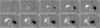 |
Fig. 1. Selected HMI images of the normal component, Bz, of the photospheric field of eruptive AR 11422 taken during the interval given in Table 1. All images are saturated at ±1900 G. The length of the horizontal white line corresponds to 150″. |
In all cases, the AR formation was accompanied by the separation of magnetic polarities over time, as is clearly shown in Figs. 1–4. This is one of the most traditional signatures of magnetic flux emergence (e.g., see the discussion in van Driel-Gesztelyi & Green 2015, and in references therein). In the vicinity of the AR polarity inversion lines (PIL), the most common motion included the shearing along the PIL, as shown in Figs. 1–4. Rotation of magnetic polarities is also occasionally observed (e.g., in Fig. 2, see the evolution of the western sunspot from panel e to panel j), and so are magnetic cancellation and converging motions (e.g., see the gradual disappearance of the magnetic patches south of the western sunspot of Fig. 1 from panel d to panel h, as well as the weakening of the eastermost positive and negative magnetic patches from panel f to panel h of Fig. 2). All these motions may inject or redistribute free magnetic energy and helicity into the system; we refer to Patsourakos et al. (2020) for a recent review of the relevant physical mechanisms.
Before computing the magnetic helicity and energy budgets of the ARs, we evaluated their rate of magnetic flux emergence, r, as well as their maximum magnetic flux content, Φmax. The first was calculated at the interval, Δt, where magnetic flux was rising monotonically. If the magnetic fluxes at the start and end of that interval are Φ1 and Φ2, respectively, then r = (Φ2 − Φ1)/Δt. The flux emergence rate lay in the interval [0.6, 10.9] × 1016 Mx s−1, in agreement with previous results (e.g., see Otsuji et al. 2011), and its mean value was (4.0 ± 2.4)×1016 Mx s−1. We note that the eruptive ARs were associated with somewhat higher magnetic flux emergence rates than the noneruptive ARs ((5.6 ± 1.9)×1016 Mx s−1 and (3.7 ± 2.5) × 1016 Mx s−1, respectively). The uncertainties reported here are the root mean square (rms) of the r and Φmax (see below) distributions.
The maximum magnetic flux of the ARs lay in the range of [0.9, 34.3] × 1021 Mx, and their mean value was (8.9 ± 7.5)×1021 Mx. In most cases, flux emergence was followed by an extended interval (usually lasting until the end of the observations) with smaller magnetic flux changes (see the top panels of Figs. 5, 6, and 8). However, at the low-end part of the Φmax distribution, there are ARs whose decay starts well before the end of the observations. One example, AR 11143, is given in Figs. 3 and 7; the magnetic flux time profile of Fig. 7 starts decreasing less than 12 h after it attained magnetic flux maximum. However, these regions cannot qualify as ephemeral ARs because they last longer and contain more magnetic flux than typical ephemeral ARs (according to the traditional definition provided by Harvey & Martin 1973, ephemeral ARs last 1–2 days and contain magnetic flux of about 1020 Mx). The high-end part of the Φmax distribution is populated by ARs that produce CMEs or/and flares. For example, the mean value of the maximum magnetic flux of the ARs that produced CMEs was (20.2 ± 9.2)×1021 Mx.
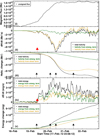 |
Fig. 5. Time profiles of the magnetic flux, helicity, and energy for eruptive AR 11422. (i) Time evolution of the unsigned magnetic flux of eruptive AR 11422. (ii) Time profile of the helicity injection rate, dH/dt (black). The gold and green curves represent the shear and emergence terms, respectively. (iii) The corresponding time profiles of accumulated helicity, ΔH(t). (iv) Same as panel (ii), but for the magnetic energy injection rate, dE/dt. (v) Same as panel (iii), but for the accumulated energy, ΔE. The red and black arrows indicate the start time of the CME and flares above C1.0, respectively, that occurred in the AR. The curves of both dH/dt and dE/dt are 48 min averages of the actual curves. |
Seven ARs produced CMEs (see Table 1); furthermore, 16 ARs produced flares with an X-ray class above C1.0 (all 7 ARs that produced CMEs also produced flares above C1.0). We are interested in the first CME produced by the ARs here; in two cases, these CMEs were associated with M-class flares, and in five cases, they were associated with C-class flares. The total number of flares above C1.0 was 98; of these, 83 (i.e., about 85%) occurred during either the flux emergence interval or around the time of maximum magnetic flux. This is clearly shown in the examples of Figs. 5 and 6 (see the location of the black arrows above the time axis). This result agrees with previous publications (e.g., see van Driel-Gesztelyi & Green 2015, and references therein). On the other hand, five CMEs occurred during either the flux emergence interval (see Fig. 5 for an example) or around the time of maximum magnetic flux, and the remaining two occurred well after the AR attained its maximum magnetic flux (see Fig. 6 for an example). Overall, flares tend to occur earlier than CMEs: the first flare (CME) occurs on average 1.6 (3.2) days after the start of flux emergence. These results are consistent with the well-known fact (e.g., see Démoulin et al. 2002) that CMEs may occur at any stage during the evolution of ARs.
The signs of the magnetic helicity budgets that we derived are reliable. This statement is made because there is extensive discussion about the most suitable magnetic helicity flux density proxy (e.g., see Pariat et al. 2005, 2006; Dalmasse et al. 2014, 2018). Although different proxies may yield different helicity flux density distributions for a given data set, the total helicity flux (which is the quantity that we record) remains the same (Pariat et al. 2005; Dalmasse et al. 2014).
The majority of ARs have negative helicity in the northern hemisphere and positive helicity in the southern hemisphere; this is the so-called hemispheric helicity rule that was first postulated by Hale et al. (1919) and was rediscovered by Seehafer (1990) and Pevtsov et al. (1995). Although this rule is well established (see Park et al. 2020, for more recent references), a rather limited number of publications have appeared (e.g., see Smyrli et al. 2010) that studied the possible changes (or the absence thereof) of the helicity sign during the evolution of individual ARs. Our calculations provide the opportunity to examine this issue and its possible relation with flares and CMEs.
The first question in this problem is the temporal scale. Because our data set consists of emerging ARs, it appears reasonable to first compare the sign of the accumulated helicity during the emergence interval, ΔHemerg, against the helicity, ΔHW45 accumulated throughout the tracking interval, that is, from flux emergence start time until the AR crosses W45. We found that in 45 out of the 52 ARs the sign did not change (see panel iii of Figs. 5 and 7), whereas in 7 ARs it did change (see panel iii of Figs. 6 and 8). In the latter cases, the sign change resulted from the sign change in helicity injection rate (see panel ii of Figs. 6 and 8). In 13 of the 45 ARs, we registered intervals longer than 6 h with an opposite sign of the helicity injection rate. This did not affect the final signs of either ΔHemerg or ΔHW45. In most of the 7 + 13 = 20 ARs the sign change in helicity injection rate occurred during the emergence interval. This result is broadly consistent with that reported by Liu et al. (2014), who found that 43% of their sample of 28 emerging ARs showed a change in helicity injection rate sign during emergence.
Of the 45 ARs with a stable helicity sign, 35 (∼78%) obeyed the hemispheric helicity rule. If we take the whole sample into account, the signs of ΔHemerg or ΔHW45 obey the hemispheric helicity rule in 39 and 38 ARs (75% and 73%), respectively. The percentages we found agree with the results reported by Park et al. (2020) for the ascending phase of solar cycle 24.
From the populations of 7 and 16 ARs that produced CMEs and ≥C1-class flares, respectively (see above), 6 and 13 ARs, respectively, showed stable signs of accumulated helicity in the sense of the previous discussion (see Fig. 5 and 6 for an example and counterexample, respectively). Their percentages are similar to the corresponding percentages of the general population of ARs. We note that at the time at which all CMEs and flares that were registered occured in the ARs (with the minor exception of two C-class flares from AR 11465; see Fig. 6), the sign of the helicity injection rate was the same as that of the corresponding ΔHemerg or ΔHW45 value, whichever was relevant. Overall, our results do not show any evidence for an impulsive injection of helicity of opposite sign, in disagreement with a few previous reports (e.g., see Moon et al. 2002). This conclusion does not change even if we consider the dH/dt curves prior to their smoothing. We also note that by analyzing a large data set of ARs, Park et al. (2021) have found that the highest flaring activity tends to occur in heliographic regions that follow the hemispheric helicity rule only little. We were not able to check this finding because our data set contained too few ARs that were all observed during the early phase of cycle 24.
We also studied the contribution of the shear term and emergence term of Eqs. (1) and (2) to the magnetic helicity and energy accumulated into the corona. We found that in our ARs, the shear term contributes 83% of the helicity and 45% of the energy on average in terms of their absolute values, while the emergence term contributes 17% of the helicity and 55% of the energy on average. This situation is reflected in panels ii–iv of Figs. 5–8, where the time profiles of the shear and emerging term contributions to the dH/dt, ΔH, dE/dt, and ΔE are given by the gold and green curves, respectively. These results are consistent with those reported by Liu & Schuck (2012), Liu et al. (2014). We refer to these papers for the interpretation of the results.
5. Magnetic helicity–energy diagram
5.1. Magnetic helicity and energy thresholds for eruptivity
From our magnetic energy and helicity computations we constructed scatter plots of the accumulated amount of these quantities. In general, our computations do not provide instantaneous values of these budgets (cf. Sect. 3 for the relevant discussion of the helicity budgets acquired before any CME activity), therefore the intervals in which the accumulated budgets are assessed for the scatter plots can in principle be selected arbitrarily. However, in order to treat the budgets in the same way, it is reasonable to use two intervals for each AR (see Cols. (4)–(7) of Table 1) that both start from the beginning of the observations and end (i) at the end of the flux emergence phase, and (ii) at the time when the AR produces its first CME or crosses W45, whichever occurs first. For each eruptive AR, interval (ii) is therefore bounded by the start time of observations and the time of CME occurrence, while for each noneruptive AR, it corresponds to the whole observation period. The absolute values of these amounts are reported in Cols. (4)–(7) of Table 1, and the corresponding scatter plots are presented in Fig. 9. The selection of intervals (i) is justified by the fact that they represent an important common evolutionary stage that is exhibited by all ARs, while intervals (ii) are the longest intervals for which the accumulated helicities of eruptive ARs correspond to instantaneous helicity budgets. If there is no CME, intervals (ii) yield the terminal budgets of both magnetic helicity and energy.
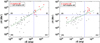 |
Fig. 9. Scatter plots of the accumulated amounts of magnetic energy vs. absolute helicity during the flux emergence intervals of the ARs (left panel) and during the intervals from emergence start times until the ARs cross W45 or produce their first CME, whichever occurs first (right panel). The red squares and black crosses correspond to eruptive and noneruptive ARs, respectively. The blue dashed lines define the thresholds for magnetic helicity and energy above which ARs show a high probability to erupt. The green lines show the least-squares best logarithmic fits (Eqs. (4) and (5)). |
The plots of Fig. 9 (hereafter referred to as E–H diagrams) show an overall trend (albeit with some scatter that may partly arise from the fact that the intervals employed for the calculations of the accumulated quantities changed over the sample of ARs) under which both magnetic helicity and energy increase together. The least-squares best logarithmic fits are
 (4)
(4)
and
 (5)
(5)
for the pairs of the left and right panel of Fig. 9, respectively. Equations (4) and (5) have significance levels of the Kolmogorov–Smirnov statistic of about 0.70 and 0.86, respectively. We note that the magnetic helicity, H – free energy, Ec, diagram constructed by Tziotziou et al. (2012) from instantaneous values of these quantities was fitted with a scaling of the form  with a Kolmogorov–Smirnov significance level of about 0.7.
Probably the most important feature of the scatter plots of Fig. 9 is that the eruptive ARs tend to appear in the top right part of the E–H diagrams. The trend is better visible in the left panel, where the ΔEemerg vs. ΔHemerg scatter plot is presented. In it, all seven eruptive ARs have helicity and energy budgets above 9 × 1041 Mx2 and 2 × 1032 erg, respectively.
These threshold values for the magnetic helcity and energy divide each plot of Fig. 9 into four regions, marked (i)–(iv). The vast majority of ARs lie in regions (i) and (iii), which contain populations with high (low) helicity and high (low) magnetic energy, respectively. This reflects the overall monotonic magnetic energy–helicity dependence. In both panels of Fig. 9, regions (ii) and (iv) contain fewer ARs, which may be a consequence of either the typical scatter in the E–H diagram or of the appearance of ARs with a comparable amount of both senses of helicity, respectively. The very small number of points in regions (iv) indicates that in a statistical sense, most ARs that are highly charged with magnetic energy exhibit a well-defined dominant sense of helicity (see also Pariat et al. 2006; Tziotziou et al. 2012).
The helicity threshold we derived is consistent with that derived by Tziotziou et al. (2012), which was 2 × 1042 Mx2. Furthermore, our inferred threshold for magnetic helicity is broadly consistent with the maximum likelihood value of the helicity distribution of magnetic clouds, which is 6.3 × 1042 Mx2, according to Patsourakos & Georgoulis (2016), who compiled calculations published by Lynch et al. (2003) and Lepping et al. (2006). Due to the conserved nature of helicity, the magnetic cloud helicity is considered as a proxy to the helicity carried away by its parent CME. This argument is supported by the overall agreement between the helicities of the source region and the associated magnetic cloud (although with significant uncertainties; e.g., see Green et al. 2002; Nindos et al. 2003; Luoni et al. 2005; Mandrini et al. 2005; Kazachenko et al. 2012).
Tziotziou et al. (2012) derived a magnetic free energy threshold of 4 × 1031 erg, which is a factor of 5 smaller than ours. Here two remarks are in place. First, our calculations of the magnetic energy injection rate include both its free and potential parts (see Liu & Schuck 2012; Liu et al. 2014). Second, during any given interval, the ARs dissipate magnetic free energy in various quantities, ranging from the weakest microflares whose detection limit is determined by the specifications of the instrument (see Nindos et al. 2020, for previous and recent references) to, possibly, flares above C1.0 and CMEs. In a study of AR microflares that were observed by the Ramaty High Energy Solar Spectroscopic Imager (RHESSI), Christe et al. (2008) found that their power was lower than 1026 erg s−1 on average. If we take into account that the first CME in our eruptive ARs occurred 3.2 days after the start of flux emergence on average, we conclude that the weak flaring events that occurred in this interval may require an amount of energy lower than 2.8 × 1031 erg. In addition to this energy, one should take into account the energy required by possible flares above C1.0. In terms of the released energy, the most flare-productive AR of our data set was AR 11158 (see Tziotziou et al. 2013, for a study of its magnetic helicity and energy budgets) which generated two C-class (C1.1 and C4.7) and an M6.6-class flare before its first CME. Shibata et al. (2013) argued that the energy of a C1.0, M1.0, and X1.0 class flare is roughly 1029, 1030, and 1031 erg, respectively. With these rough estimates, the total energy content of the three flares was about 7.2 × 1030 erg. If we add the amount required for the small events, the amount is 3.5 × 1031 erg. Aschwanden et al. (2014) studied several large flares and reported that the ratio of the free magnetic energy to the potential energy may range from 0.01 to 0.25. Therefore our magnetic energy threshold could broadly accommodate both the free magnetic energy required for flaring activity and the underlying potential energy.
The appearance of the eruptive ARs in the top right corner of the E–H diagrams indicates that ARs with an accumulated magnetic helicity and energy above 9 × 1041 Mx2 and 2 × 1032 erg are more likely to erupt than those ARs that contain lower values of accumulated magnetic helicity and energy. We used the ϕ coefficient to evaluate the statistical signifant of this result. This coefficient is related to χ2 values via χ2 = nϕ2 (e.g., see Klimov 1986) (n is 52, i.e., the number of ARs), which can then be compared to tabulated values of χ2 with one degree of freedom. For the data appearing in the left panel of Fig. 9, we found χ2 = 44.83, which means that the null hypothesis (i.e., that the production of a CME and the strength of the magnetic helicity and energy in an AR are not correlated) can be rejected at the 100% confidence level. For the data of the right panel of Fig. 9, we found χ2 = 25.25, and the null hypothesis can be rejected at the 99.999997% confidence level. We note that if only one of the thresholds (no matter which) is taken into account and the values of either panel of Fig. 9 are used, the null hypothesis is also rejected at a confidence level of about 99.999%. This means that each threshold, even if taken separately, can serve as a reliable indicator of AR eruptivity. This result is consistent with previous results on AR eruptivity, which highlight either the central role of the magnetic energy (e.g., see Priest 2014, and references therein) or solely invoke a magnetic helicity threshold (see Sect. 1 for references).
We also calculated an E–H diagram similar to the diagram presented in the right panel of Fig. 9, but instead of the absolute value of the accumulated helicity, |ΔH|, we used the magnetic flux-normalized absolute helicity, |ΔH|/Φ2, where Φ is the magnetic flux when the AR crosses W45 or produces its first CME. To first approximation, this quantity reflects the structure of the magnetic field, while ΔH reflects both the structure and the magnetic flux content (the helicity of an isolated, uniformly twisted magnetic flux tube with N turns and magnetic flux Φ is NΦ2). The results of our computations are shown in Fig. 10. The degree of segregation of the eruptive ARs from the noneruptive ARs is similar to the degree in Fig. 9. This visual impression is confirmed by our statistical analysis, which shows that by using ΔH/Φ2, the null hypothesis is again rejected at a confidence level of ∼99.9999%. In Fig. 10 all eruptive ARs exhibit |ΔH|/Φ2 in the range [0.014, 0.096]. These values are consistent with those reported in the literature (e.g., see Patsourakos et al. 2020, and references therein).
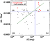 |
Fig. 10. Same as the right panel of Fig. 9, but the magnetic flux-normalized absolute accumulated helicity (|ΔH|/Φ2) is presented instead of |ΔH|. |
Some authors (e.g., Pariat et al. 2017; Thalmann et al. 2019) have argued that both helicity and magnetic flux-normalized helicity are poor indicators of the AR approach to the threshold of instability and only the ratio of current-carrying to total helicity is a good indicator. The study by Pariat et al. (2017) can be understood as an attempt to address the question of whether there is a well-defined value of flux-normalized helicity that completely segregates eruptive from noneruptive ARs; all of the ARs should erupt above a certain value. In this sense, we tested a weaker hypothesis, namely, whether there is a well-defined value of ΔH (or ΔH/Φ2) above which ARs are more likely to erupt. Figure 10 shows that the likelihood of an eruption increases above ΔH/Φ2 = 0.014 because it is zero below this value. In this sense, ΔH/Φ2 behaves absolutely similarly to ΔH. However, when ΔH/Φ2 lies in the range of about [0.014, 0.028] , no clear statement about the eruptivity of the ARs can be made because this range is populated by significant fractions of eruptive and noneruptive ARs. Therefore, ΔH/Φ2 does not possess a critical value that completely segregates the stability domain from the instability domain. Our results indicate that a range of ΔH/Φ2 values may exist that includes this boundary. In this sense, our results partially agree with the relevant conclusion of Pariat et al. (2017).
We conclude this subsection with some remarks about the uncertainties of the magnetic helicity and energy calculations. The uncertainties in the calculations of dH/dt and dE/dt were evaluated using selected pairs of vector magnetic field data that yielded representative values of dH/dt and dE/dt (from 1035 to 1038 Mx2 s−1 for the helicity flux and from 1025 to 1028 erg s−1 for the energy flux). Briefly, we used the Monte Carlo experiment approach described by Liu & Schuck (2012) and Liu et al. (2014) and found that the relative errors quantified by the ratio of the standard deviation σdH/dt (or σdE/dt) to the absolute value of the mean dH/dt (or dE/dt, respectively) increased as the mean magnetic helicity or energy flux values decreased (see Park et al. 2020), but they never exceeded 30%. The resulting errors in the accumulated helicity or energy were almost two orders of magnitude smaller than the relevant accumulated quantity. These results are consistent with those reported by Liu & Schuck (2012) and indicate that the uncertainties in our calculations could not challenge the location of the ARs in the E–H diagrams of Figs. 9 and 10 with respect to the helicity (either total or flux normalized) and energy thresholds.
5.2. Deviations
The segregation of the eruptive ARs from the noneruptive ARs in the E–H diagrams of Fig. 9 is not complete. The left panel of Fig. 9 shows three noneruptive ARs that are located in region (i) of the E–H diagram. The right panel of Fig. 9 shows one eruptive AR (NOAA 11422; see Fig. 1) that is located in region (iii), which is populated by the vast majority of the noneruptive ARs, and there are also six noneruptive ARs in region (i) of the diagram. In this subsection we investigate possible reasons for these deviations.
The appearance of AR 11422 in region (iii) in the right panel of Fig. 9 is a direct consequence of the occurrence of its CME early on in the flux emergence phase (about 1.4 days from the flux emergence start time; see Fig. 5) before the AR accumulates significant magnetic helicity and energy budgets. Although this is the only AR of our sample that exhibited this behavior, it is well known (e.g., see Nitta & Hudson 2001; Nindos & Zhang 2002; Zhang & Wang 2002) that occasionally, ARs can produce major eruptions early in their flux emergence phase.
For the six ARs that intrude into region (i) in the right panel of Fig. 9, we investigated whether the overlying background magnetic field inhibited eruptions. It is well known that a magnetic flux rope tends to erupt due to the Lorentz self-force (Chen 1989), but the overlying field provides the restraining Lorentz force to keep the balance of the flux rope. If the overlying magnetic field decreases fast with height, then the so-called torus instability develops (Kliem & Török 2006), which may lead to a CME. The rate at which the overlying field decreases with height is quantified by its decay index, n, defined by
 (6)
(6)
where Bh is the horizontal component ( ) of the overlying field and z is the height above the photosphere. The nominal critical decay index for the initiation of the torus instability of a magnetic flux rope is nc ≈ 1.5 (Kliem & Török 2006; Olmedo & Zhang 2010; Cheng et al. 2011).
For each AR we calculated the decay index at the end time of the interval used for the production of the right panel of Fig. 9, that is, the time of the first CME if the AR is eruptive or the time of W45 crossing if the AR is noneruptive. The first step in the computation was to extrapolate the coronal magnetic field using the observed photospheric Bz magnetograms as boundary conditions. Because we were interested in the large-scale structure of the overlying field, we employed potential extrapolations using the method by Alissandrakis (1981) (we note that Nindos et al. 2012, have shown that to first approximation, potential and nonlinear force-free field extrapolations yield similar decay index trends). The size of the base of the extrapolation volume was equal to the size of the Bz magnetogram and its height was 160 Mm. The decay index was computed using Eq. (6), and the extrapolated field within a computation box whose base encompassed the main polarity inversion line of the AR and its height was the height of the extrapolation volume. For each height, the average value of the decay index was used in our study.
In Fig. 11 we show scatter plots of the accumulated budgets of magnetic helicity and enery that were registered in the right panel of Fig. 9 vs. the height at which the decay index reached the critical value of 1.5. This value is relevant when a magnetic flux rope becomes torus unstable, whereas we did not investigate the existence of magnetic flux ropes in our ARs. However, even if some ARs lack flux ropes, the comparison of the heights at which the decay indices reach a common reference value, nc, may provide information about the restraining potential of the overlying field. Figure 11 shows that both the magnetic helicity and energy budgets spread all over the nc heights. However, the noneruptive ARs of region (i) in the right panel of Fig. 9 tend to acquire nc = 1.5 at larger heights (> 60 Mm) than most eruptive ARs (compare the locations of the red boxes and the green diamonds). The same conclusion is reached if the flux-normalized accumulated helicity is used instead of the accumulated helicity because the noneruptive ARs in the top right quarter of Figs. 9 (right) and 10 are largely the same; the scatter plot of ΔH/Φ2 vs. critical height is very similar to the bottom panel of Fig. 11 regarding the segregation of the green diamonds from the red squares. Our result indicates that in ARs with significant helicity and energy budgets, the background field tends to provide stronger confinement in the ARs that did not produce CMEs than in those that produce a CME. Our result is broadly consistent with the work by Vasantharaju et al. (2018), who studied 77 flare-CME events and reported that in 90% of eruptive flares the decay index reached nc = 1.5 within 42 Mm, while it was beyond 42 Mm in ∼70% of confined flares.
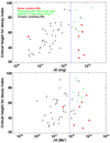 |
Fig. 11. Scatter plots of accumulated magnetic energy and helicity vs. critical height for decay index. Top: accumulated magnetic energy from emergence start times until the ARs produce their first CME or cross W45, whichever occurs first, vs. height at which the decay index that has been calculated at the end of the intervals that were used to determine the magnetic energy budgets, reaches a value of 1.5. Red boxes denote eruptive ARs, and green diamonds denote the noneruptive ARs that appear in region (i) in right panel of Fig. 9. All other ARs are marked by crosses. Bottom panel: same as the top panel, but for the magnetic helicity instead of the magnetic energy. |
6. Summary and conclusions
We computed the magnetic helicity and energy injection rates as well as the resulting accumulated budgets of 52 emerging ARs over intervals that start at the flux emergence start time and end when the ARs cross W45. The instantaneous helicity is very low when flux emergence starts, and therefore the conservation of helicity in the corona dictates that the accumulated helicity budgets provide estimates of the instantaneous helicity content of an AR at any time until the possible occurrence of the first CME. On the other hand, this is not the case for the magnetic energy, which is dissipated due to reconnection events.
During the tracking intervals, 7 ARs produced CMEs and 45 did not. All but one of the CME-producing ARs exhibited sign-unchanging budgets of accumulated helicity during the computations. For one of these ARs (AR 11560), this was first noted by Vemareddy (2015). We also note that in the one eruptive AR of our sample that exhibited helicity sign change during the observations, the CME occurred well after the sign reversal (see Fig. 6), allowing the AR to accumulate significant helicity and energy budgets.
For each AR, we further assessed the accumulated magnetic helicity and energy budgets in two intervals: (i) the flux emergence phase, and (ii) the interval until the first CME if the AR was eruptive, or the whole observing period if the AR was not eruptive. The results appear in Cols. (4)–(7) of Table 1 and in more concise form in Table 2. The produced E–H diagrams (Fig. 9) show a partial segregation of the eruptive ARs from the noneruptive ARs; the former tend to appear in the top right part of the scatter plots, which reflects their larger budgets of magnetic helicity and energy. The same conclusion was reached when we considered the flux-normalized helicity instead of the helicity.
Mean and median values of accumulated magnetic helicities and energies.
The E–H diagrams indicate that if magnetic helicity and energy thresholds of 9 × 1041 Mx2 and 2 × 1032 erg, are crossed, ARs are likely to erupt. The helicity threshold is consistent with the one derived by Tziotziou et al. (2012) using instantaneous helicity budgets as well as with published reports of the helicity contents of CMEs and magnetic clouds. On the other hand, the high value of the magnetic energy threshold reflects both the noninstantaneous nature of its budgets and the fact that these budgets contain not only the free magnetic energy, but also the potential energy. The magnetic energy threshold may account for the potential energy contribution and the dissipation of energy due to reconnection events throughout the interval until the first CME.
The segregation of the eruptive from the noneruptive ARs in the E–H diagrams is not perfect. The sources of the violations are as follows:
-
(1)
In one case, an AR erupts early on during its emergence phase without having the opportunity to accumulate significant helicity and energy budgets. It is possible that the eruption occurred as a result of reconnection between the newly emerged flux and the preexisting flux of an AR located ∼60″ west of the emergence site.
-
(2)
In six cases, ARs exhibit high magnetic helicity and energy budgets, but do not erupt. The computation of the decay index for all ARs at the end times of the intervals used for the assembly of the E–H diagram revealed that the six outlier ARs acquire the critical decay index, nc = 1.5, at heights above 60 Mm, whereas six out of seven eruptive ARs acquire it at heights below 60 Mm. Therefore it is possible that the six outlier ARs did not erupt because the overlying magnetic field provided stronger or more extended confinement than in eruptive ARs.
The first statistical study of the magnetic helicity and energy injection in emerging ARs was performed by Liu et al. (2014). Our paper is the first statistical study of the eruptive behavior of emerging ARs in terms of their accumulated magnetic helicity and energy. We found that in a statistical sense, the erupting ARs possess larger budgets of both these quantities. A similar result for ARs producing major flares (M and X class) has been reported by Tziotziou et al. (2012). The new ingredients of our study compared to that of Tziotziou et al. (2012) are listed below.
-
(1)
We employed a different magnetic helicity and energy calculation method (flux-integration method vs. connectivity-based method).
-
(2)
Our data base consisted exclusively of emerging ARs, which are known to produce flares during the flux emergence phase.
-
(3)
Only in two ARs were the CMEs associated with M-class flares; in the remaining five ARs, the CMEs were associated with C-class flares.
We conclude that the finding that emerging ARs that erupt statistically accumulate more magnetic helicity and energy than noneruptive ARs is a robust result. This means that magnetic helicity and magnetic energy in any study of the eruptive potential of these ARs should be treated equally.
Acknowledgments
We thank the referee for his/her constructive comments. We thank C.E. Alissandrakis, S. Patsourakos, and K. Moraitis for useful discussions. EL acknowledges partial financial support from University of Ioannina’s internal grant 82561/81698/β6.ϵ. YL was supported by NASA LWS program (award No. 80NSSC19K0072).
References
- Alissandrakis, C. E. 1981, A&A, 100, 197 [NASA ADS] [Google Scholar]
- Archontis, V., & Syntelis, P. 2019, Phil. Trans. R. Soc. London Ser. A, 377, 20180387 [Google Scholar]
- Aschwanden, M. J., Xu, Y., & Jing, J. 2014, ApJ, 797, 50 [Google Scholar]
- Berger, M. A. 1984, Geophys. Astrophys. Fluid Dyn., 30, 79 [NASA ADS] [CrossRef] [Google Scholar]
- Berger, M. A. 1999, Magnetic Helicity in Space Physics (USA: American Geophysical Union), 111, 1 [Google Scholar]
- Bobra, M. G., Sun, X., Hoeksema, J. T., et al. 2014, Sol. Phys., 289, 3549 [Google Scholar]
- Boerner, P., Cheung, C., Schrijver, C., Testa, P., & Weber, M. 2012, AGU Fall Meeting Abstracts, SH33B [Google Scholar]
- Chae, J. 2001, ApJ, 560, L95 [NASA ADS] [CrossRef] [Google Scholar]
- Chen, J. 1989, ApJ, 338, 453 [NASA ADS] [CrossRef] [Google Scholar]
- Cheng, X., Zhang, J., Ding, M. D., Guo, Y., & Su, J. T. 2011, ApJ, 732, 87 [NASA ADS] [CrossRef] [Google Scholar]
- Choudhary, D. P., Gosain, S., Gopalswamy, N., et al. 2013, AdSpR, 52, 1561 [NASA ADS] [Google Scholar]
- Christe, S., Hannah, I. G., Krucker, S., McTiernan, J., & Lin, R. P. 2008, ApJ, 677, 1385 [NASA ADS] [CrossRef] [Google Scholar]
- Dalmasse, K., Pariat, E., Démoulin, P., & Aulanier, G. 2014, Sol. Phys., 289, 107 [NASA ADS] [CrossRef] [Google Scholar]
- Dalmasse, K., Pariat, É., Valori, G., Jing, J., & Démoulin, P. 2018, ApJ, 852, 141 [NASA ADS] [CrossRef] [Google Scholar]
- Démoulin, P., Mandrini, C. H., van Driel-Gesztelyi, L., et al. 2002, A&A, 382, 650 [NASA ADS] [CrossRef] [EDP Sciences] [Google Scholar]
- Dhakal, S. K., Zhang, J., Vemareddy, P., & Karna, N. 2020, ApJ, 901, 40 [NASA ADS] [CrossRef] [Google Scholar]
- Gary, G. A., & Hagyard, M. J. 1990, Sol. Phys., 126, 21 [Google Scholar]
- Georgoulis, M. K., & LaBonte, B. J. 2007, ApJ, 671, 1034 [NASA ADS] [CrossRef] [Google Scholar]
- Georgoulis, M. K., Tziotziou, K., & Raouafi, N.-E. 2012, ApJ, 759, 1 [NASA ADS] [CrossRef] [Google Scholar]
- Gopalswamy, N., Yashiro, S., Michalek, G., et al. 2009, Earth Moon Planets, 104, 295 [NASA ADS] [CrossRef] [Google Scholar]
- Green, L. M., López fuentes, M. C., Mandrini, C. H., et al. 2002, Sol. Phys., 208, 43 [Google Scholar]
- Guo, Y., Pariat, E., Valori, G., et al. 2017, ApJ, 840, 40 [NASA ADS] [CrossRef] [Google Scholar]
- Hale, G. E., Ellerman, F., Nicholson, S. B., & Joy, A. H. 1919, ApJ, 49, 153 [NASA ADS] [CrossRef] [Google Scholar]
- Harvey, K. L., & Martin, S. F. 1973, Sol. Phys., 32, 389 [NASA ADS] [CrossRef] [Google Scholar]
- Hoeksema, J. T., Liu, Y., Hayashi, K., et al. 2014, Sol. Phys., 289, 3483 [Google Scholar]
- Kazachenko, M. D., Canfield, R. C., Longcope, D. W., & Qiu, J. 2012, Sol. Phys., 277, 165 [NASA ADS] [CrossRef] [Google Scholar]
- Kliem, B., & Török, T. 2006, Phys. Rev. Lett., 96, 255002 [Google Scholar]
- Klimov, G. 1986, Probability Theory and Mathematical Statistics (Moscow: Mir Publishers) [Google Scholar]
- Kusano, K., Maeshiro, T., Yokoyama, T., & Sakurai, T. 2002, ApJ, 577, 501 [NASA ADS] [CrossRef] [Google Scholar]
- Kusano, K., Yokoyama, T., Maeshiro, T., & Sakurai, T. 2003, AdSpR, 32, 1931 [NASA ADS] [Google Scholar]
- Kusano, K., Maeshiro, T., Yokoyama, T., & Sakurai, T. 2004, ApJ, 610, 537 [NASA ADS] [CrossRef] [Google Scholar]
- LaBonte, B. J., Georgoulis, M. K., & Rust, D. M. 2007, ApJ, 671, 955 [CrossRef] [Google Scholar]
- Leka, K. D., Canfield, R. C., McClymont, A. N., & van Driel-Gesztelyi, L. 1996, ApJ, 462, 547 [NASA ADS] [CrossRef] [Google Scholar]
- Lemen, J. R., Title, A. M., Akin, D. J., et al. 2012, Sol. Phys., 275, 17 [Google Scholar]
- Lepping, R. P., Berdichevsky, D. B., Wu, C. C., et al. 2006, Ann. Geophys., 24, 215 [Google Scholar]
- Liu, Y., & Schuck, P. W. 2012, ApJ, 761, 105 [NASA ADS] [CrossRef] [Google Scholar]
- Liu, Y., & Schuck, P. W. 2013, Sol. Phys., 283, 283 [NASA ADS] [CrossRef] [Google Scholar]
- Liu, Y., Hoeksema, J. T., Bobra, M., et al. 2014, ApJ, 785, 13 [NASA ADS] [CrossRef] [Google Scholar]
- Low, B. C. 1996, Sol. Phys., 167, 217 [Google Scholar]
- Luoni, M. L., Mandrini, C. H., Dasso, S., van Driel-Gesztelyi, L., & Démoulin, P. 2005, J. Atmos. Solar-Terrest. Phys., 67, 1734 [NASA ADS] [CrossRef] [Google Scholar]
- Lynch, B. J., Zurbuchen, T. H., Fisk, L. A., & Antiochos, S. K. 2003, J. Geophys. Res. (Space Physics), 108, 1239 [NASA ADS] [CrossRef] [Google Scholar]
- Mandrini, C. H., Pohjolainen, S., Dasso, S., et al. 2005, A&A, 434, 725 [NASA ADS] [CrossRef] [EDP Sciences] [Google Scholar]
- Moon, Y. J., Chae, J., Wang, H., Choe, G. S., & Park, Y. D. 2002, ApJ, 580, 528 [NASA ADS] [CrossRef] [Google Scholar]
- Nindos, A., & Andrews, M. D. 2004, Astrophys. J. Lett., 616, L175 [NASA ADS] [CrossRef] [Google Scholar]
- Nindos, A., & Zhang, H. 2002, ApJ, 573, L133 [NASA ADS] [CrossRef] [Google Scholar]
- Nindos, A., Zhang, J., & Zhang, H. 2003, ApJ, 594, 1033 [Google Scholar]
- Nindos, A., Patsourakos, S., & Wiegelmann, T. 2012, ApJ, 748, L6 [Google Scholar]
- Nindos, A., Alissandrakis, C. E., Patsourakos, S., & Bastian, T. S. 2020, A&A, 638, A62 [NASA ADS] [CrossRef] [EDP Sciences] [Google Scholar]
- Nitta, N. V., & Hudson, H. S. 2001, Geophys. Res. Lett., 28, 3801 [NASA ADS] [CrossRef] [Google Scholar]
- Olmedo, O., & Zhang, J. 2010, ApJ, 718, 433 [NASA ADS] [CrossRef] [Google Scholar]
- Otsuji, K., Kitai, R., Ichimoto, K., & Shibata, K. 2011, PASJ, 63, 1047 [Google Scholar]
- Pariat, E., Démoulin, P., & Berger, M. A. 2005, A&A, 439, 1191 [NASA ADS] [CrossRef] [EDP Sciences] [Google Scholar]
- Pariat, E., Nindos, A., Démoulin, P., & Berger, M. A. 2006, A&A, 452, 623 [NASA ADS] [CrossRef] [EDP Sciences] [Google Scholar]
- Pariat, E., Valori, G., Démoulin, P., & Dalmasse, K. 2015, A&A, 580, A128 [NASA ADS] [CrossRef] [EDP Sciences] [Google Scholar]
- Pariat, E., Leake, J. E., Valori, G., et al. 2017, A&A, 601, A125 [CrossRef] [EDP Sciences] [Google Scholar]
- Park, S.-H., Lee, J., Choe, G. S., et al. 2008, ApJ, 686, 1397 [NASA ADS] [CrossRef] [Google Scholar]
- Park, S.-H., Chae, J., & Wang, H. 2010, ApJ, 718, 43 [NASA ADS] [CrossRef] [Google Scholar]
- Park, S.-H., Leka, K. D., & Kusano, K. 2020, ApJ, 904, 6 [NASA ADS] [CrossRef] [Google Scholar]
- Park, S.-H., Leka, K. D., & Kusano, K. 2021, ApJ, 911, 79 [NASA ADS] [CrossRef] [Google Scholar]
- Patsourakos, S., & Georgoulis, M. K. 2016, A&A, 595, A121 [NASA ADS] [CrossRef] [EDP Sciences] [Google Scholar]
- Patsourakos, S., Vourlidas, A., Török, T., et al. 2020, Space Sci. Rev., 216, 131 [Google Scholar]
- Pesnell, W. D., Thompson, B. J., & Chamberlin, P. C. 2012, Sol. Phys., 275, 3 [Google Scholar]
- Pevtsov, A. A., Canfield, R. C., & Metcalf, T. R. 1995, ApJ, 440, L109 [NASA ADS] [CrossRef] [Google Scholar]
- Pevtsov, A. A., Maleev, V. M., & Longcope, D. W. 2003, ApJ, 593, 1217 [NASA ADS] [CrossRef] [Google Scholar]
- Pevtsov, A. A., Berger, M. A., Nindos, A., Norton, A. A., & van Driel-Gesztelyi, L. 2014, Space Sci. Rev., 186, 285 [NASA ADS] [CrossRef] [Google Scholar]
- Phillips, A. D., MacNeice, P. J., & Antiochos, S. K. 2005, ApJ, 624, L129 [NASA ADS] [CrossRef] [Google Scholar]
- Priest, E. 2014, Magnetohydrodynamics of the Sun (Cambridge: Cambridge University Press) [Google Scholar]
- Sammis, I., Tang, F., & Zirin, H. 2000, ApJ, 540, 583 [Google Scholar]
- Scherrer, P. H., Schou, J., Bush, R. I., et al. 2012, Sol. Phys., 275, 207 [Google Scholar]
- Schmieder, B., Archontis, V., & Pariat, E. 2014, Space Sci. Rev., 186, 227 [NASA ADS] [CrossRef] [Google Scholar]
- Schou, J., Scherrer, P. H., Bush, R. I., et al. 2012, Sol. Phys., 275, 229 [Google Scholar]
- Schrijver, C. J. 2009, AdSpR, 43, 739 [NASA ADS] [Google Scholar]
- Schuck, P. W. 2008, ApJ, 683, 1134 [NASA ADS] [CrossRef] [Google Scholar]
- Schunker, H., Braun, D. C., Birch, A. C., Burston, R. B., & Gizon, L. 2016, A&A, 595, A107 [NASA ADS] [CrossRef] [EDP Sciences] [Google Scholar]
- Seehafer, N. 1990, Sol. Phys., 125, 219 [NASA ADS] [CrossRef] [Google Scholar]
- Shibata, K., Isobe, H., Hillier, A., et al. 2013, PASJ, 65, 49 [NASA ADS] [Google Scholar]
- Smyrli, A., Zuccarello, F., Romano, P., et al. 2010, A&A, 521, A56 [NASA ADS] [CrossRef] [EDP Sciences] [Google Scholar]
- Sun, X. 2013, ArXiv e-prints [arXiv:1309.2392] [Google Scholar]
- Thalmann, J. K., Moraitis, K., Linan, L., et al. 2019, ApJ, 887, 64 [Google Scholar]
- Thalmann, J. K., Georgoulis, M. K., Liu, Y., et al. 2021, ApJ, 922, 41 [NASA ADS] [CrossRef] [Google Scholar]
- Toriumi, S. 2014, PASJ, 66, S6 [NASA ADS] [CrossRef] [Google Scholar]
- Toriumi, S., & Wang, H. 2019, Liv. Rev. Sol. Phys., 16, 3 [Google Scholar]
- Tziotziou, K., Georgoulis, M. K., & Raouafi, N.-E. 2012, ApJ, 759, L4 [NASA ADS] [CrossRef] [Google Scholar]
- Tziotziou, K., Georgoulis, M. K., & Liu, Y. 2013, ApJ, 772, 115 [Google Scholar]
- Valori, G., Pariat, E., Anfinogentov, S., et al. 2016, Space Sci. Rev., 201, 147 [Google Scholar]
- van Driel-Gesztelyi, L., & Green, L. M. 2015, Liv. Rev. Sol. Phys., 12, 1 [Google Scholar]
- Vasantharaju, N., Vemareddy, P., Ravindra, B., & Doddamani, V. H. 2018, ApJ, 860, 58 [NASA ADS] [CrossRef] [Google Scholar]
- Vemareddy, P. 2015, ApJ, 806, 245 [NASA ADS] [CrossRef] [Google Scholar]
- Vemareddy, P. 2017, ApJ, 845, 59 [NASA ADS] [CrossRef] [Google Scholar]
- Vemareddy, P. 2019, ApJ, 872, 182 [NASA ADS] [CrossRef] [Google Scholar]
- Zhang, J., & Wang, J. 2002, ApJ, 566, L117 [Google Scholar]
- Zhang, M., Flyer, N., & Low, B. C. 2006, ApJ, 644, 575 [NASA ADS] [CrossRef] [Google Scholar]
- Zhang, Y., Zhang, M., & Zhang, H. 2008, Sol. Phys., 250, 75 [Google Scholar]
- Zhang, M., Flyer, N., & Chye Low, B. 2012, ApJ, 755, 78 [NASA ADS] [CrossRef] [Google Scholar]
- Zirin, H. 1988, Astrophysics of the sun (Cambridge: Cambridge University Press) [Google Scholar]
All Tables
All Figures
|
Fig. 1. Selected HMI images of the normal component, Bz, of the photospheric field of eruptive AR 11422 taken during the interval given in Table 1. All images are saturated at ±1900 G. The length of the horizontal white line corresponds to 150″. |
| In the text | |
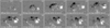 |
Fig. 2. Same as Fig. 1, but for eruptive AR 11465. |
| In the text | |
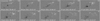 |
Fig. 3. Same as Fig. 1, but for noneruptive AR 11143. |
| In the text | |
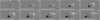 |
Fig. 4. Same as Fig. 1, but for noneruptive AR 11327. |
| In the text | |
|
Fig. 5. Time profiles of the magnetic flux, helicity, and energy for eruptive AR 11422. (i) Time evolution of the unsigned magnetic flux of eruptive AR 11422. (ii) Time profile of the helicity injection rate, dH/dt (black). The gold and green curves represent the shear and emergence terms, respectively. (iii) The corresponding time profiles of accumulated helicity, ΔH(t). (iv) Same as panel (ii), but for the magnetic energy injection rate, dE/dt. (v) Same as panel (iii), but for the accumulated energy, ΔE. The red and black arrows indicate the start time of the CME and flares above C1.0, respectively, that occurred in the AR. The curves of both dH/dt and dE/dt are 48 min averages of the actual curves. |
| In the text | |
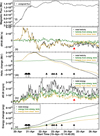 |
Fig. 6. Same as Fig. 5, but for eruptive AR 11465. |
| In the text | |
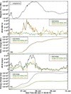 |
Fig. 7. Same as Fig. 5, but for noneruptive AR 11143. |
| In the text | |
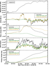 |
Fig. 8. Same as Fig. 5, but for noneruptive AR 11327. |
| In the text | |
|
Fig. 9. Scatter plots of the accumulated amounts of magnetic energy vs. absolute helicity during the flux emergence intervals of the ARs (left panel) and during the intervals from emergence start times until the ARs cross W45 or produce their first CME, whichever occurs first (right panel). The red squares and black crosses correspond to eruptive and noneruptive ARs, respectively. The blue dashed lines define the thresholds for magnetic helicity and energy above which ARs show a high probability to erupt. The green lines show the least-squares best logarithmic fits (Eqs. (4) and (5)). |
| In the text | |
|
Fig. 10. Same as the right panel of Fig. 9, but the magnetic flux-normalized absolute accumulated helicity (|ΔH|/Φ2) is presented instead of |ΔH|. |
| In the text | |
|
Fig. 11. Scatter plots of accumulated magnetic energy and helicity vs. critical height for decay index. Top: accumulated magnetic energy from emergence start times until the ARs produce their first CME or cross W45, whichever occurs first, vs. height at which the decay index that has been calculated at the end of the intervals that were used to determine the magnetic energy budgets, reaches a value of 1.5. Red boxes denote eruptive ARs, and green diamonds denote the noneruptive ARs that appear in region (i) in right panel of Fig. 9. All other ARs are marked by crosses. Bottom panel: same as the top panel, but for the magnetic helicity instead of the magnetic energy. |
| In the text | |
Current usage metrics show cumulative count of Article Views (full-text article views including HTML views, PDF and ePub downloads, according to the available data) and Abstracts Views on Vision4Press platform.
Data correspond to usage on the plateform after 2015. The current usage metrics is available 48-96 hours after online publication and is updated daily on week days.
Initial download of the metrics may take a while.