| Issue |
A&A
Volume 662, June 2022
|
|
|---|---|---|
| Article Number | A67 | |
| Number of page(s) | 22 | |
| Section | Interstellar and circumstellar matter | |
| DOI | https://doi.org/10.1051/0004-6361/202142769 | |
| Published online | 17 June 2022 | |
Importance of source structure on complex organics emission
I. Observations of CH3OH from low-mass to high-mass protostars
1
Leiden Observatory, Leiden University,
PO Box 9513,
2300
RA Leiden,
The Netherlands
e-mail: This email address is being protected from spambots. You need JavaScript enabled to view it.
2
Max Planck Institut für Extraterrestrische Physik (MPE),
Giessenbachstrasse 1,
85748
Garching,
Germany
3
INAF – Osservatorio Astrofisico di Arcetri,
Largo E. Fermi 5,
50125
Firenze,
Italy
4
Jodrell Bank Centre for Astrophysics, Department of Physics and Astronomy, University of Manchester,
Oxford Road,
Manchester
M13 9PL,
UK
5
I. Physikalisches Institut, Universität zu Köln,
Zülpicher Str.77,
50937
Köln,
Germany
6
RIKEN Cluster for Pioneering Research, Wako-shi,
Saitama
351-0106,
Japan
7
Department of Astronomy, University of Virginia,
Charlottesville,
VA
22904-4235,
USA
Received:
27
November
2021
Accepted:
8
February
2022
Abstract
Context. Complex organic molecules (COMs) are often observed toward embedded Class 0 and I protostars. However, not all Class 0 and I protostars exhibit COM emission.
Aims. The aim is to study variations in methanol (CH3OH) emission and use this as an observational tracer of hot cores to test if the absence of CH3OH emission can be linked to source properties.
Methods. A sample of 148 low-mass and high-mass protostars is investigated using new and archival observations with the Atacama Large Millimeter/submillimeter Array (ALMA) that contain lines of CH3OH and its isotopologues. Data for an additional 36 sources are added from the literature, giving a total of 184 different sources. The warm (T ≳ 100 K) gaseous CH3OH mass, MCH3OH, is determined for each source using primarily optically thin isotopologues and is compared to a simple toy model of a spherically symmetric infalling envelope that is passively heated by the central protostar.
Results. A scatter of more than four orders of magnitude is found for MCH3OH among the low-mass protostars, with values ranging between 10−7 M⊙ and ≲10−11 M⊙. On average, Class I protostellar systems seem to have less warm MCH3OH(≲10−10 M⊙) than younger Class 0 sources (~10−7 M⊙). High-mass sources in our sample show more warm MCH3OH, up to ~10−7−10−3 M⊙. To take into account the effect of the source’s overall mass on MCH3OH, a normalized CH3OH mass is defined as MCH3OH/Mdust,0, where Mdust,0 is the cold plus warm dust mass in the disk and inner envelope within a fixed radius measured from the ALMA dust continuum. A correlation between MCH3OH/Mdust,0 and Lbol is found. Excluding upper limits, a simple power-law fit to the normalized warm CH3OH masses results in MCH3OH/Mdust,0 ∝ Lbol0.70±0.05 over an Lbol range of 10−1−106 L⊙. This is in good agreement with the toy model, which predicts that the normalized MCH3OH increases with Lbol0.70 due to the snow line moving outward. Sources for which the size of the disk is equivalent to or smaller than the estimated 100 K radius fall within the 3σ range of the best-fit power-law model, whereas sources with significantly larger disks show normalized warm CH3OH masses that are up to two orders of magnitude lower.
Conclusions. The agreement between sources that are rich in CH3OH with the toy model of a spherically symmetric infalling envelope implies that the thermal structure of the envelopes in these sources is likely not strongly affected by a disk. However, based on the disagreement between the toy model and sources that show less warm CH3OH mass, we suggest that source structure such as a disk can result in colder gas and thus fewer COMs in the gas phase. Additionally, optically thick dust can hide the emission of COMs. Advanced modeling is necessary to quantify the effects of a disk and/or continuum optical depth on the presence of gaseous COMs in young protostellar systems.
Key words: astrochemistry / stars: formation / stars: protostars / techniques: interferometric / ISM: molecules
© ESO 2022
1 Introduction
Complex organic molecules (COMs), molecules with six or more atoms (see Herbst & van Dishoeck 2009; Jørgensen et al. 2020, for reviews), are commonly observed toward both low-mass and high-mass young embedded protostellar systems (e.g., Belloche et al. 2013; Ceccarelli et al. 2014; Jørgensen et al. 2016; Bøgelund et al. 2019; van Gelder et al. 2020; Nazari et al. 2021; Yang et al. 2021). They are also detected in protostellar outflows (e.g., Arce et al. 2008; Codella et al. 2017; Tychoniec et al. 2021) and in low abundances in cold clouds (Bacmann et al. 2012; Scibelli et al. 2021; Jiménez-Serra et al. 2021). The simplest COMs, such as methanol (CH3OH) and methyl cyanide (CH3CN), have also been detected toward more evolved low-mass Class II systems (Walsh et al. 2014; Öberg et al. 2015), in some cases hinting at an inheritance between pre-stellar cores and protoplanetary disks (Booth et al. 2021; van der Marel et al. 2021). It is particularly important to assess the chemical complexity during the embedded Class 0/I phases of star formation since planet formation is thought to start early (e.g., Harsono et al. 2018; Manara et al. 2018; Alves et al. 2020; Tychoniec et al. 2020).
The earliest Class 0 and I phases are also most suitable for studying COMs in the gas phase since the temperatures in the inner hot cores are high enough to sublimate COMs from ices (e.g., van ‘t Hoff et al. 2020). However, not all Class 0 and I sources show emission from COMs, even when observed at high sensitivity with interferometers such as the Atacama Large Millimeter/submillimeter Array (ALMA) and the Northern Extended Millimeter Array (NOEMA). Yang et al. (2021) find that CH3OH, the most abundant COM, is present in only 56% of the 50 surveyed embedded sources in Perseus. Similarly, Belloche et al. (2020) detect emission from CH3OH toward 50% of the 26 low-mass protostars in their sample. A main question remains as to why some embedded sources show emission of COMs while others do not.
One possible explanation for the absence of gaseous COM emission could be the presence of a disk that casts a shadow on the inner envelope and therefore decreases the temperature throughout the system (Persson et al. 2016; Murillo et al. 2015, 2018). Most COMs will then likely be frozen out in the inner envelopes and cold midplanes of these disks. For low-mass sources in the Class 0 phase, these disks are usually small (< 10–50 au; Segura-Cox et al. 2018; Maury et al. 2019), but larger disks of up to ~ 100 au have also been observed (e.g., Tobin et al. 2012; Murillo et al. 2013; Sakai et al. 2019). Around more evolved Class I systems, larger disks are more common (e.g., Harsono et al. 2014; Yen et al. 2017; Artur de la Villarmois et al. 2019), although some Class I sources still also show small disks of < 10 au (Segura-Cox et al. 2018). Furthermore, disk-like structures seem to be present around some high-mass protostars (e.g., Sánchez-Monge et al. 2013; Johnston et al. 2015; Ilee et al. 2016; Maud et al. 2019; Zhang et al. 2019; Moscadelli et al. 2021), but not all (Beltrán & de Wit 2016). The effect of a disk on the presence of COM emission, however, remains largely unknown.
Alternatively, optically thick dust at (sub)millimeter wavelengths can hide the emission of COMs in protostellar systems. This was recently shown to be the case in NGC 1333 IRAS4A1, where De Simone et al. (2020) used the Very Large Array (VLA) to show that this source, which was thought to be poor in COMs based on observations with ALMA (López-Sepulcre et al. 2017), has emission of CH3OH at centimeter wavelengths. Similarly, Rivilla et al. (2017) found high dust opacities affecting the molecular lines of COMs toward the high-mass source G31.41+0.31.
Some sources may also be intrinsically deficient in COMs, although this is not expected based on the large columns of CH3OH ice observed toward pre-stellar and starless cores (e.g., Chu et al. 2020; Goto et al. 2021) and many protostellar systems (Pontoppidan et al. 2003; Boogert et al. 2008; Öberg et al. 2011; Bottinelli et al. 2010; Perotti et al. 2020, 2021). Furthermore, recent chemical models of the collapse from pre-stellar core to protostellar system do not show a significant destruction of COMs, including CH3OH (Drozdovskaya et al. 2014; Aikawa et al. 2020).
In this work, the amount of warm CH3OH is determined for a large sample of 148 sources, covering both low-mass and high-mass protostellar systems. Furthermore, literature values of an additional 36 sources are collected, giving a total sample of 184 sources. The goal is to determine, from an observational point of view, how source structures, such as a disk or optically thick dust, affect gaseous COM emission. Optically thin isotopologues of CH3OH are used to mitigate line optical depth effects. The reduction of the ALMA data sets used in this work and the determination of the amount of warm CH3OH from the ALMA observations are described in Sect. 2. The results are presented in Sect. 3 and discussed in Sect. 4. Our main conclusions are summarized in Sect. 5. In this paper, the amount of warm CH3OH is only compared to a simple analytic toy model of a spherically symmetric infalling envelope passively heated by the luminosity of the protostar; a full comparison to sophisticated disk plus envelope models that include dust optical depth effects is presented in a companion paper (Nazari et al. 2022).
2 Methodology
2.1 Observations and archival data
The data analyzed in this work consist of a combination of multiple ALMA data sets that encompass 148 different sources. These data sets are all taken in Band 6 (~1.2 mm) but in different setups, covering different transitions of CH3OH and its 13C and 18O isotopologues. Moreover, the observations are taken with different beam sizes and sensitivities, and the observed sources are located at various distances, which need to be taken into account in the analysis (see Sect. 2.3). The full list of sources and their observational properties are presented in Table A.1.
The reduction of the 2017.1.01174.S (PI: E.F. van Dishoeck) data set, which contains four protostars in Perseus and three in Serpens, is described by van Gelder et al. (2020). Only the Band 6 data with a 0.45” beam, which contain transitions of both the 13C and 18O isotopologues of CH3OH, are used in this work. Three out of seven sources in this program show emission from COMs. For Serpens SMM3, archival pipeline imaged product data are used from the 2017.1.01350.S (PI: Ł. Tychoniec) program (Tychoniec et al. 2021).
In total, 50 protostars in Perseus were observed in the Perseus ALMA Chemistry Survey (PEACHES) in programs 2016.1.01501.S and 2017.1.01462.S (PI: N. Sakai). The goal of this program is to probe the complex chemistry toward embedded protostars in Perseus at ~0.4” (i.e., 150 au) scales. The full list of PEACHES sources is presented in Table A.1. The reduction and imaging of the PEACHES data are described in detail by Yang et al. (2021). Only two transitions of  are covered at low spectral resolution (~1.2 km s−1). Furthermore, the PEACHES data contain three transitions of 13CH3OH, of which the 259.03649 GHz line is blended with HDCO for most COM-rich sources. Several strong transitions of the main CH3OH isotopologue, which likely produce optically thick lines, are covered. All PEACHES sources were also observed in the VLA Nascent Disk and Multiplicity Survey (VANDAM), which showed that ~50% of the Class 0 and ~20% of the Class I sources are part of multiple systems (Tobin et al. 2016). Moreover, the presence of disks at >10 au scales around several Perseus sources was presented by Segura-Cox et al. (2018).
The ALMA Evolutionary study of High Mass Protocluster Formation in the Galaxy (ALMAGAL) survey (2019.1.00195.L; PI: S. Molinari) is a large program that targeted over 1000 dense clumps with M > 500 M⊙ and d < 7.5 kpc in Band 6. The ALMAGAL sources were targeted based on compact sources within the Herschel Hi-GAL survey (Molinari et al. 2010; Elia et al. 2017, 2021). In this paper, a subsample of 40 high-mass protostellar cores has been selected based on a combination of high bolometric luminosity (≳1000 L⊙) and richness in spectral lines. Moreover, only archival data with a beam size smaller than 2″ (~ 1000−5000 au) that were public in February 2021 are included. As discussed below, this selection introduces a bias. The data are pipeline-calibrated and imaged with Common Astronomy Software Applications1 (CASA; McMullin et al. 2007) version 5.6.1. The ALMAGAL data cover multiple transitions of (likely) optically thick CH3OH, four transitions of 13CH3OH, and nine transitions of  . Especially for the line-rich sources with broad lines, many of these lines are unfortunately affected by line blending.
The integrated intensity maps of CH3OH are presented in Fig. 1 for a few representative sources: B1-c from the 2017.1.01174.S program, Per-emb 13 (NGC 1333 IRAS 4B) from PEACHES, and 881427 from ALMAGAL. For B1-c and Per-emb 13, some outflow emission is evident, but this does not influence the analysis below. The position of the continuum emission peak for all sources is listed in Table A.1, and the peak continuum flux within the central beam for each source is listed in Table A.2. All spectra are extracted from the central pixel on the continuum peak positions.
Several of the sources used in this work (e.g., 881427 in Fig. 1) are resolved into small clusters in the higher-resolution ALMA images (see Table A.1). However, their luminosity is often estimated from Herschel observations within a ~15″ beam (Murillo et al. 2016; Elia et al. 2017, 2021), and therefore luminosity estimates of the individual cores are unknown. In such cases, as a zeroth-order approximation, the luminosity of each individual core was estimated by dividing the luminosity over the multiple sources. The fraction attributed to each source was computed as the peak continuum flux of the corresponding core divided by the sum of peak continuum fluxes from all cores.
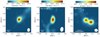 |
Fig. 1 Integrated intensity maps of the CH3 OH 21,1−10,1 line for the low-mass protostar B1-c (left), the CH3OH 51,4−41,3 line for the low-mass protostar Per-emb 13 from PEACHES (middle), and the CH3OH 80,8−71,6 line for the high-mass 881427 cluster (right). The color scale is shown on top of each image. The images are integrated over [−5,5] km s−1 with respect to the Vlsr. The white vertical line in the colorbar indicates the 3σ threshold. The peaks in the continuum are indicated with the white stars. The white ellipse in the lower right of each image depicts the beam size, and in the lower left a physical scale bar is displayed. |
2.2 Deriving the column density
The column density of  , was calculated from the spectrum through local thermodynamic equilibrium models using the spectral analysis tool CASSIS2 (Vastel et al. 2015). Since spectral lines originating from the main isotopologue of CH3OH are likely optically thick, lines from optically thin iso-topologues such as 13CH3OH and
  need to be invoked to get an accurate estimate of the column density. The 12C/13C and 16O/18O ratios are dependent on the galactocentric distance and are determined using the relations of Milam et al. (2005) and Wilson & Rood (1994), respectively. For the local interstellar medium, this results in ratios of 12C/13C ~ 70 and 16O/18O ~ 560. The full line lists were acquired from the CDMS catalog3 (Müller et al. 2001, 2005; Endres et al. 2016) and are presented for each data set in Appendix B.
For the PEACHES and ALMAGAL data sets, generally only a few lines of each isotopologue are detected. Therefore, for simplicity, an excitation temperature of Tex = 150 K was assumed, which is roughly the average of what is observed toward both low-mass and high-mass protostellar systems (typical values lie in the range of 100-300 K; e.g., Bøgelund et al. 2018, 2019; van Gelder et al. 2020; Yang et al. 2021). Changing the excitation temperature within the 100-300 K range leads to only a factor of ~2 variation in the derived column densities since lines with a range of Eup from ~50 to ~800 K are available for the analysis. The column density, N, of each isotopologue is derived separately using a grid fitting method similar to that presented in van Gelder et al. (2020), with N and the full width at half maximum (FWHM) of the line as free parameters. The size of the emitting region was set equal to the beam size and is presented for each source in Table A.2. To exclude emission associated with outflows, only narrow lines (FWHM ≲ few km s−1 ) with Eup ≳ 50 K were used in the analysis. Moreover, blended lines were excluded from the fit. The 2σ uncertainty on N was derived from the grid. Careful inspection by eye was conducted to test the validity of the fits and derived column densities.
In Fig. 2, fits to lines of CH3OH and its isotopologues are presented for Per-emb 13 from the PEACHES sample and 881427C from the ALMAGAL sample. All lines in Fig. 2 are >3σ detections. The  lines suffer from line blending in 881427C as well as in many other PEACHES and ALMAGAL sources. Since all other lines originating from 13CH3OH in the PEACHES data suffer from line blending (e.g., with HDCO), the 13CHзOH 233,20−232,21 (Eup = 675 K) line in Fig. 2 often provides the only constraint on the column density.
The derived CH3OH column densities are presented in Table A.2. The column densities of the sources in the 2017.1.01174.S and 2017.1.01350.S data sets were derived by van Gelder et al. (2020). Only the Band 6 results are used in this work. When no lines originating from  were detected, the column density of CH3OH was derived from 13CH3OH lines. In cases where only upper limits on the column densities of both 13CH3OH and
  could be derived,
  was calculated by setting the 3σ upper limit based on scaling the 3σ upper limit of 13CH3OH and the lower limit based on the main iso-topologue. This situation results in rather large error bars on
  for 9 low-mass and 25 high-mass sources. When the main isotopologue of CH3OH is also not detected, the 3σ upper limit is reported. The upper limits on
  are not homogeneous across the full sample since they are derived from various ALMA programs with a range of sensitivities covering different transitions of CH3OH with different upper energy levels and Einstein Aij coefficients. For sources with detections, this inho-mogeneity is not present, except for the uncertainty based on the assumed Tex.
Besides the sources presented in Table A.1, other sources with or without warm (T ≳ 100 K) CH3OH detections are also included from the literature. These sources include well-known low-mass hot cores, such as IRAS 16293-2422 (Jørgensen et al. 2016, 2018; Manigand et al. 2020), NGC 1333 IRAS4A (De Simone et al. 2020), BHR 71 (Yang et al. 2020), and L438 (Jacobsen et al. 2019), but also sources with disks that show emission of COMs, such as HH 212 (Lee et al. 2017b, Lee et al. 2019a), and outbursting sources, such as SVS 13A (Bianchi et al. 2017; Hsieh et al. 2019) and V883 Ori (van ‘t Hoff et al. 2018; Lee et al. 2019b). Non-detections of CH3OH, such as found for several Class I sources in Ophiuchus, are also included (Artur de la Villarmois et al. 2019). Moreover, classical high-mass hot cores, such as AFGL 4176 (Bøgelund et al. 2019), NGC 63341 (Bøgelund et al. 2018), and Sgr B2 (Belloche et al. 2013; Müller et al. 2016; Bonfand et al. 2017), are taken into account. A 20% uncertainty on  was assumed for literature sources where no uncertainty on the column density was reported. The full list of literature sources is also presented in Table A.2. Including the 36 literature sources, the total sample studied in this work contains 184 unique sources (some sources, such as Bl-bS and Per-emb 44 (SVS 13A), are covered in both our data and literature studies).
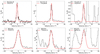 |
Fig. 2 Spectral line fits of CH3OH (left), 13CH3OH (middle), and |


2.3 Calculating the warm methanol mass
In order to get a measurement of the amount of warm (T ≳ 100 K) CH3OH gas, observational dependences should be taken into account. Column densities provide a measure of the amount of CH3OH, but they depend on the assumed size of the emitting region. From the 184 sources studied in this work, ~30 (mostly high-mass) sources show spatially resolved CH3OH emission; nevertheless, in these cases most of the CH3OH emission is still located within the central beam. Furthermore, emission from 13CH3OH and  , which gives more stringent constraints on
  , is only spatially resolved in a few high-mass sources. Therefore, in this work the size of the emitting region is assumed to be equal to the size of the beam. Because our sample consists of many different types of sources at a range of distances taken with different ALMA programs, all derived column densities were multiplied by the physical area of the beam to derive the total number of CH3OH molecules,
  , within the beam,
 (1)
(1)
Here,  is the observed column density in the beam and Rbeam is the physical radius of the beam,
 (2)
(2)
with d the distance to the source and θbeam the angular size of the beam. For some of the literature sources, the adopted emitting region is different from the beam size (e.g., Bianchi et al. 2017; Jacobsen et al. 2019). In these cases, the assumed size of the emitting region was adopted in the computation of  (see the θS0Urce column in Table A.2). However, it is important to note that the assumed size of the emitting region does not alter the resulting value of
  as long as the beam-averaged column density is derived from optically thin lines (i.e., from the 13C or 18O isotopologues). If the lines are optically thick, this approach provides a lower limit on
  Finally, the warm gaseous CH3OH mass,
  , was computed through
 (3)
(3)
where  is the molar mass of a methanol molecule of 5.32 × 10⁻²³ g or 2.67 × 10−56 M⊙.
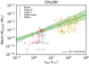 |
Fig. 3 Warm CH3OH mass as a function of the bolometric luminosity. Different colors denote different observational classes, and all sources with Lbol > 1000 L are classified as highmass sources. Additionally, sources that are suggested to currently be in a burst phase (e.g., V883 Ori and IRAS 2A; van ’t Hoff et al. 2018; Lee et al. 2019b; Hsieh et al. 2019) are highlighted. Sources in the “other” category include Class II and flat spectrum sources. The green line indicates the best-fit power-law model to the data points (excluding the upper limits) and the green shaded area the 3 uncertainty on the fit. |
3 Results
3.1 Amount of warm methanol from low to high mass
The derived values of  are presented in Table A.2 for all sources. In Fig. 3,
  is plotted as a function of the bolo-metric luminosity, Lbol A clear trend in
  as a function of Lbol is evident: more luminous sources have more CH3OH in the gas phase. Excluding upper limits, a simple power-law fit to the results gives a
  relation, which is presented in Fig. 3 along with the 3σ uncertainty on the fit. The positive correlation found here agrees well with that found for low-mass Class 0 protostars in Orion (Hsu et al. 2022). The positive correlation is in line with the expectation that
  increases with Lbol since sources with a higher luminosity are expected to have their CH3OH snow line at larger radii, which results in more CH3OH in the gas phase. Furthermore, the envelopes of sources with higher Lbol are more massive and thus contain more CH3OH mass in the first place. However, the result of the fit strongly depends on the difference in warm
  between the low-mass (Lbol ≲ 100 L⊙) and high-mass (Lbol ≳ 1000 L⊙) protostars. Fitting these two subsamples individually gives a weaker correlation between
  and Lbol (
 and
and  for low-mass and high-mass protostars, respectively). Due to the large uncertainties on the fits of both subsamples, no significant conclusions can be made.
For the lower-mass sources (Lbol ≲ 100 L⊙), a scatter of more than four orders of magnitude is present. On average, Class 0 sources seem to show more CH3OH mass (~10−7 M⊙) compared to more evolved Class I sources (≲10−10 M⊙). In fact, for the majority of the Class I sources, only upper limits can be derived on  (e.g., the Class I sources in Ophiuchus; Artur de la Villarmois et al. 2019), but some Class I sources do show emission of COMs, including CH3OH (e.g., L1551 IRS5; Bianchi et al. 2020). Moreover, known bursting sources, such as IRAS 2A (or Per-emb 27; Hsieh et al. 2019; Yang et al. 2021) and V883 Ori (van’t Hoff et al. 2018; Lee et al. 2019b), show a large amount of CH3OH mass despite the presence of disk-like structures (Segura-Cox et al. 2018; Maury et al. 2019).
The high-mass (Lbol ≳ 1000 L⊙) sources show higher gaseous CH3OH masses (i.e., 10−7−10−3 M⊙) compared to the lower-mass sources. A similar scatter of about four orders of magnitude is present, but fewer sources seem to show lower CH3OH masses. This is likely a sample bias effect since mostly very line-rich sources from the ALMAGAL data set are analyzed, whereas many ALMAGAL sources show upper limits. Hence, in reality, more sources with  will be present among the high-mass sources as well. Alternatively, the emitting region in high-mass sources could be larger than the typical disk sizes reached, resulting in fewer sources for which the disk has a significant effect on the thermal structure.
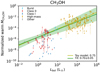 |
Fig. 4 Normalized warm gaseous CH3OH mass, |

3.2 Comparison to spherically symmetric Mailing envelope
To quantify the effect of the luminosity on the amount of warm methanol, a simple toy model of a spherically symmetric infalling envelope was constructed (see Appendix C). In this simple toy model, the warm methanol mass is linked to Lbol,
 (4)
(4)
where M0 is the total warm plus cold mass contained within a reference radius, R0. As qualitatively discussed in Sect. 3.1, the warm methanol mass is thus dependent on both the envelope mass within a reference radius (or, alternatively, the density at a reference radius) and the luminosity of the source. The former is straightforward since a higher mass will result in a higher initial methanol mass. The latter is the result of the snow line of CH3OH moving to larger radii for larger luminosities.
Hence, to probe the effect of the luminosity on the snow line radius in our observations, the values of  presented in Sect. 3.1 should be divided by a reference mass, M0, defined within a reference radius, R0. The protostellar envelope mass, Menv, is not as good an option as M0 since it is not consistently constrained for many sources and depends on the adopted outer radius (e.g., Kristensen et al. 2012). Therefore, in this work the dust mass within a common arbitrary radius of 200 au, denoted as Mdust,0, is used as the reference mass. The computation of Mdust,o from the continuum flux is detailed in Appendix D, and the derived values are reported in Table A.2. The choice for R0 = 200 au is based on it being larger than the typical disk size of low-mass protostars. Despite 200 au being smaller than the typical size of a high-mass hot core, we do not expect this to influence our analysis since the scale on which the continuum flux is measured (>1000 au) is dominated by the envelope. Furthermore, the continuum flux on 200 au scales is not filtered out in either the PEACHES or ALMAGAL observations.
In Fig. 4, the normalized warm gaseous CH3OH mass,  , is presented as a function of Lbol. It is important to note that the
  ratio is a dimensionless quantity and does not represent an abundance of CH3OH in the system. The warm gaseous CH3OH mass was derived from a region taken to have a size similar to that of the beam. The dust mass, Mdust,0, includes both cold and warm material in the disk and envelope and is defined as the mass within the fixed radius, Ro = 200 au. For most low-mass sources, the snow line is expected to be well within 200 au, whereas for high-mass sources the snow line is at radii larger than 200 au. However, changing the normalization to larger or smaller R0 does not affect the results discussed below.
Despite  not representing an abundance of CH3OH, it can be seen as a lower limit on the abundance of CH3OH in the hot cores of sources where the expected snow line radius lies inward of 200 au (i.e., when Lbol ≲ 100 L⊙). For typical values of
  , this implies abundances of ≳10−7 with respect to H2 (assuming a gas-to-dust mass ratio of 100), which is in agreement with the CH3OH ice abundances in protostellar envelopes (~10−6 with respect to H2; Boogert et al. 2008; Bottinelli et al. 2010; Öberg et al. 2011).
A positive correlation of  with Lbol is evident,
  (again excluding upper limits). The slope of the power law is in good agreement with the slope derived in Eq. (4) for the simple toy model (yellow line in Fig. scaled to match the best-fit power-law mode). This indicates that for sources with high
  the thermal structure of the envelope is likely not affected by the disk. Since the sources are corrected for the source’s mass, the increase in the
  ratio originates from the snow line moving farther out in systems with higher luminosity. In turn, this leads to a higher mass of gaseous warm CH3OH. Therefore, the agreement with the toy model can be considered as an observational confirmation of the scaling between the sublimation radius (i.e., the snow line radius) and the source luminosity of
  found in radiative transfer calculations (i.e., Eq. (C.3); Bisschop et al. 2007; van’t Hoff et al. 2022).
The correlation between  and Lbol is most evident when the low-mass and high-mass samples are combined. A positive correlation is less evident when the two subsam-ples are examined individually:
  and
and  for the low-mass and high-mass protostars, respectively. However, the uncertainties on the fits are large due to the large scatter within each subsample. Moreover, the fits are more sensitive to individual data points (e.g., B1-bS at low Lbol). Therefore, no significant conclusions can be made.
Similarly to Fig. 3, a scatter of more than four orders of magnitude is evident in Fig. 4 among both the low-mass and high-mass sources. Likewise, on average, the Class I sources show lower values  than the (younger) Class 0 sources
  . The large scatter indicates that the normalized gaseous CH3OH mass cannot be solely explained by the toy model of a spherically symmetric infalling envelope.
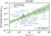 |
Fig. 5 Normalized warm gaseous CH3OH mass with respect to Mdust within a 200 au radius as a function of the bolometric luminosity. Sources around which a disk has been detected on >10 au scales are indicated in blue, and sources where no disk is confirmed on >50 au scales are indicated in red. All other sources (i.e., with no information about a disk) are shown in gray. The green line indicates the best-fit power-law model to the data points (excluding the upper limits) and the green shaded area the 3σ uncertainty on the fit. The yellow line indicates the relation for the toy model of Eq. (4) scaled to match the best-fit power-law model. |
4 Discussion
4.1 Importance of source structure
If all embedded protostellar systems behaved solely as spherically symmetric infalling envelopes, a larger luminosity for a given mass of the source would result in the CH3OH snow line moving farther out and, thus, more CH3OH in the gas phase. However, the large scatter in Fig. 4 indicates that other mechanisms affect the gaseous CH3OH mass. One possible explanation could be the presence of a disk that alters the temperature structure of the system and thus lowers the amount of warm CH3OH. Alternatively, the continuum optical depth can hide the emission of COMs. These cases could explain the deviation from the toy model relation of Eq. (4).
In Fig. 5, the normalized warm gaseous CH3OH mass is presented as a function of Lbol, similarly to Fig. 4 but now with colors indicating whether the source has a confirmed disk on >10 au scales (blue) or whether the absence of a > 50 au disk is confirmed. All sources where no information on the presence of a disk is available (e.g., high-mass sources) are assigned to the “other” category. Besides the sources with well-known disks, such as HH 212 (e.g., Lee et al. 2017b, 2019a), the presence of a disk is indicated by Keplerian rotation (e.g., L1527 and V883 Ori; Tobin et al. 2012; Lee et al. 2019b) or based on the elongated dust continuum (e.g., Segura-Cox et al. 2018; Maury et al. 2019).
Among the low-mass sources, the presence of a disk does not directly imply that no significant COM emission can be present, given that the emission of COMs can be in the part of the envelope not shadowed by the disk or in the warm upper atmosphere of the disk (e.g., HH 212; Lee et al. 2017b, 2019a). Excluding the lower limits for IRAS 4A1 (Per-emb 12A; De Simone et al. 2020) and L1551IRS5 (Bianchi et al. 2020), there are only seven sources in our sample with both a confirmed disk and a CH3OH detection: HH 212, Per-emb 27 (IRAS 2A), V883 Ori, Per-emb 35A (IRAS 1A), Per-emb 26 (L1448-mm), Per-emb 1 (HH211), and Per-emb 11A (IC 348 MMS). Their normalized warm CH3OH masses as well as their estimated dust disk radii are listed in Table 1.
The normalized warm  of Per-emb 27, Per-emb 35A, and Per-emb 26 lie well within the 3σ range of the best-fit power-law model in Fig. 5 (green shaded area). Similarly, the lower limit of IRAS 4A1 (VLA) also falls within this area. This suggests that for these sources the thermal structure of the envelope is not significantly affected by the disk. This suggestion is further supported by the derived radii compared to the estimated 100 K radius based on their luminosities, assuming that the thermal structure of the envelope is not dominated by the disk (see Table 1). Especially for Per-emb 27 (IRAS 2A), the disk is much smaller than the estimated 100 K radius (Rdisk = 20 au and R100K = 147 au), suggesting that indeed the disk does not significantly affect the thermal structure.
On the other hand, V883 Ori shows normalized warm  that is more than two orders of magnitude lower than the 3σ range of the best-fit power-law model in Fig. 5. Likewise, HH 212, the ranges of Per-emb 1 and Per-emb 11A, and the lower limit of L1551 IRS5 lie about an order of magnitude below the 3σ. One possible explanation for this discrepancy is the size of the disk for these sources. The large disks around V883 Ori and L1551 IRS5 compared to their estimated 100 K radii suggest that these disks have a stronger impact on the thermal structure of these sources compared to the sources discussed above, therefore lowering the amount warm gas in the inner envelope. Since both Per-emb 27 and V883 Ori are currently in an outbursting phase (e.g., Lee et al. 2019b; Hsieh et al. 2019), this cannot explain the more than one order of magnitude difference in normalized
  . For HH 212, the edge-on disk is slightly larger than the 100 K radius, but the COMs in this source are detected through very high-angular-resolution observations (~12 au) in the part of the envelope not shadowed by the disk or the disk atmosphere (Lee et al. 2017b, 2019a). The disks around Per-emb 1 and Per-emb 11A are similar in size to the estimated 100 K radius, but since the error bars on their normalized warm CH3OH masses are rather large, no further conclusions can be made.
Of the 46 sources where no disk is confirmed on >50 au scales, 26 sources fall within 3σ of the best-fit power-law model, indicating that the thermal structure in these sources is indeed not dominated by a (large) disk. However, 20 sources where no disk is confirmed on >50 au scales lie up to two orders of magnitude below the 3σ of the best-fit power-law model. One example is BHR 71, which shows a warm normalized CH3OH mass that is about an order of magnitude lower than the 3σ range of the best-fit power-law model shown in Fig. 5. Hints of a ~50 au Keplerian disk are visible in the 13CH3OH lines (Yang et al. 2020), which is roughly similar in size to the estimated 100 K radius of ~57 au (Bisschop et al. 2007). Most of the other upper limits in Fig. 5 have constraints on their disk size down to ~10 au scales due to high-angular-resolution continuum observations in, for example, the VANDAM survey (Tobin et al. 2016; Segura-Cox et al. 2018). Therefore, it is unlikely that large disks are the explanation for the low normalized warm  in these sources, but small disks that can affect the thermal structure may still be present. An alternative reason could be the dust opacity (see Sect. 4.2).
Among the high-mass sources, only AFGL 4176 is known to host a large, ~2000 au, disk (Johnston et al. 2015); additionally, it also shows a large amount of COMs in the disk, including CH3OH (Bøgelund et al. 2019). Several other high-mass sources are likely to also host large warm disks as this seems to be common at least for A- and B-type stars (Beltrán & de Wit 2016).
However, since no information on the presence or absence of disks is available for the high-mass sources, all other high-mass sources have been assigned to the “other” category.
Disk and estimated 100 K radii for sources with both a disk and CH3OH detection.
4.2 Continuum optical depth
Another way to hide large amounts of COMs is through the continuum optical depth at (sub)millimeter wavelengths. If a layer of optically thick dust is present and coincides with or is in front of the hot core, all emission from the hot core will be extincted. Alternatively, continuum over-subtraction due to the presence of bright (optically thick) continuum emission behind the methanol emission can hide CH3OH emission (e.g., Boehler et al. 2017; Rosotti et al. 2021). A recent example of a low-mass source where optically thick dust hides emission from COMs at submillimeter wavelengths is NGC 1333 IRAS4A1 (López-Sepulcre et al. 2017; De Simone et al. 2020). For high-mass sources, the effect dust opacity on the molecular line intensities of COMs toward G31.41+0.31 was shown by Rivilla et al. (2017). Optically thick dust thus does not reduce the amount of COMs present in the gas phase, but it hides the emission from the hot core at millimeter wavelengths.
As a zeroth-order approximation, the continuum optical depth toward the sources studied in this work can be quantified using the continuum flux and assuming the dust temperature, Tdust (see Eq. (2) of Rivilla et al. 2017),
 (5)
(5)
where Ωbeam is the beam solid angle and Fv is the flux density within the beam at frequency v. Here, we assume that Tdust = 30 K and Tdust = 50 K for the low-mass and high-mass sources, respectively (see Sect. 3.2).
For the PEACHES sample, the highest optical depth value at 243 GHz (i.e., 1.23 mm) is for IRAS 4A1 (i.e., Per-emb 12A, τv = 3.9), which is consistent with a non-detection of emission by CH3OH (it is in fact in absorption at millimeter wavelengths; Sahu et al. 2019) since any COM emission is extincted with a factor of ≈50. The effect of dust opacity on the normalized warm  of IRAS 4A1 is also shown in Fig. 5, where the lower limit derived at centimeter wavelengths (IRAS 4A1 (VLA); De Simone et al. 2020) is more than two orders of magnitude higher than the normalized warm
  derived from absorption lines at millimeter wavelengths (IRAS 4A1 (ALMA)). In contrast to source A, Per-emb 12B has significantly lower extinction by the dust (τv = 0.56), explaining why source B appears rich in COMs at millimeter wavelengths. Moreover, both these optical depth estimates are consistent with those derived by De Simone et al. (2020) at 143 GHz when assuming that
  for α = 2.5 (Tychoniec et al. 2020).
In the ALMAGAL sample, the effect of dust opacity is evidently visible in the source 693 050, where the CH3OH emission is ring-shaped around the continuum peak (see Fig. 6). Using Eq. (5) for a dust temperature of 50 K, the continuum optical depth is estimated to be τv = 0.68 at 219 GHz. This could explain the decrease in emission in the center, but since the optical depth is not as high as in Per-emb 12A, CH3OH is still detected outside the central beam. Similarly, the CH3OH emission peaks slightly off-source for 707 948 (τv = 0.24), but significant emission is still present within the central beam. The reason why these optical depth values are lower than for some of the PEACHES sample could be that the solid angle of the optically thick emitting region is in reality much smaller than the beam size. However, the fact that 693 050 shows ring-shaped CH3OH emission and also has the highest optical depth of the high-mass sources is a clear case of the dust attenuation reducing the emission of CH3OH.
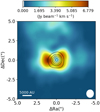 |
Fig. 6 Integrated intensity maps of the CH3OH 80,8−71,6 line for 693050. The color scale is shown on top of the image. The image is integrated over [–5,5] km s−1 with respect to the Vlsr. The white vertical line in the colorbar indicates the 3σ threshold. The continuum flux is indicated with the black contours at [0.1,0.3,0.5,0.7,0.9] times the peak continuum flux, Fcont = 1.92 Jy beam−1. The white ellipse in the lower right of each image depicts the beam size, and in the lower left a physical scale bar is displayed. |
5 Conclusion
In this work, the warm (T > 100 K) gaseous methanol mass,  , is derived for a large sample of both low-mass and highmass embedded protostellar systems. The sample includes new and archival observations of 148 sources with ALMA as well as 36 sources added from the literature, leading to a combined sample size of 184 sources. Using a simple analytic toy model of a spherically symmetric infalling envelope that is passively heated by the central protostar, the effect of source structure (e.g., a disk) and dust opacity on the amount of warm gaseous methanol is investigated. The main conclusions are as follows:
Among the low-mass protostars, a scatter of more than four orders of magnitude in
 is observed, with values ranging between 10−7 M⊙ and ≲10−11 M⊙. On average, Class 0 sources have more CH3OH mass (~10−7 M⊙) than the more evolved Class I sources (≲10−10 M⊙). High-mass sources in our biased sample show higher warm gaseous CH3OH masses, between ~10−7 and 10−3 M⊙. This scatter can be due to either source structure (e.g., the presence of a disk) or dust optical depth.
To take into account the effect of the source’s overall mass and to test the effect of the bolometric luminosity on the snow line radius, the normalized warm
 is defined as
  . Here, Mdust,0 is the cold plus warm dust mass in the disk and inner envelope within a fixed radius measured from the ALMA dust continuum. A simple power-law fit to the normalized warm
  of the line-rich sources gives a positive correlation with the bolometric luminosity:
  over an Lbol range of 10−1−106 L⊙. This in good agreement with the toy hot core model, which predicts that
  and can be considered as an observational confirmation of the scaling between the sublimation radius (i.e., snow line radius) and the source luminosity of
  found in radiative transfer calculations.
Most sources where the disk radius is equivalent to or smaller than the estimated 100 K envelope radius agree well with the power-law fit to normalized warm
 , indicating that the thermal structure of the envelope in these sources is likely not affected by the disk. On the other hand, sources for which the disk radius is significantly larger have up to two orders of magnitude lower normalized warm CH3OH masses, suggesting that these disks significantly affect the thermal structure of these sources.
High dust opacity can hide emission from COMs, leading to low observed CH3OH masses. Clear cases of this effect in our sample are the low-mass source Per-emb 12A (IRAS 4A1) and the high-mass source 693 050.
This work shows that the absence of COM emission in embedded protostellar systems does not mean that the abundance of COMs in such sources is low but instead that it may be a physical effect due to the structure of the source, most notably the presence of a disk. It is therefore very important to understand the physical structure of embedded protostellar systems in order to understand the chemistry. The modeling work done by Nazari et al. (2022) quantifies the effect that a disk has on the temperature structure of an embedded protostellar system and thus on the amount of warm methanol. Additionally, observations at longer wavelengths can solve the problem of dust optical depth.
Acknowledgements
The authors would like to thank the anonymous referee for their constructive comments on the manuscript. This paper makes use of the following ALMA data: ADS/JAO.ALMA#2017.1.01174.S, ADS/JAO.ALMA# 2017.1.01350.S, ADS/JAO.ALMA#2016.1.01501.S, ADS/JAO.ALMA#2017.1. 01462.S, and ADS/JAO.ALMA#2019.1.00195.L. ALMA is a partnership of ESO (representing its member states), NSF (USA) and NINS (Japan), together with NRC (Canada), MOST and ASIAA (Taiwan), and KASI (Republic of Korea), in cooperation with the Republic of Chile. The Joint ALMA Observatory is operated by ESO, AUI/NRAO and NAOJ. Astrochemistry in Leiden is supported by the Netherlands Research School for Astronomy (NOVA), by funding from the European Research Council (ERC) under the European Union’s Horizon 2020 research and innovation programme (grant agreement No. 101019751 MOLDISK), andbythe Dutch Research Council (NWO) grants TOP-1 614.001.751, 648.000.022, and 618.000.001. Support by the Danish National Research Foundation through the Center of Excellence “InterCat” (Grant agree-ment No.: DNRF150) is also acknowledged. G.A.F. acknowledges support from the Collaborative Research Centre 956, funded by the Deutsche Forschungsgemeinschaft (DFG) project ID 184018867. Y.-L.Y. acknowledges the support from the Virginia Initiative of Cosmic Origins (VICO) Postdoctoral Fellowship.
Appendix A Observational details
Observations of protostars.
Protostellar properties and derived physical quantities.
Appendix B Transitions of CH3OH and isotopologues
Transitions of CH3OH and isotopologues covered in the various ALMA programs.
Appendix C Toy model of a spherically symmetric infalling envelope
In this simple toy model of a spherically symmetric infalling envelope, the envelope is heated by the luminosity of the central protostar. The density structure at a radius R can be written as
 (C.1)
(C.1)
with nH,0 the density at a radius R0. The snow line radius of a molecule with sublimation temperature Tsub then scales as (for details, see Appendix B of Nazari et al. 2021)
 (C.2)
(C.2)
where γ is the slope of the temperature profile in the envelope and T0 is the temperature at a radius R0. In this work, a sublimation temperature of 100 K is adopted based on experiments of pure CH3OH and mixed H2O:CH3OH ices (e.g., Collings et al. 2004). At a typical inner envelope density of 107 cm−3, the adopted Tsub corresponds to a binding energy of ~ 5000 K, which is slightly higher than that recommended by Penteado et al. (2017). Radiative transfer calculations show that, for protostellar envelopes, γ = 2/5 at > 10 au scales and that  (Adams & Shu 1985). Equation (C.2) can then be written as
 (C.3)
(C.3)
which (except for a pre-factor) is similar to the relation that was derived by Bisschop et al. (2007) for the 100 K radius in high-mass protostars and more recently seen to be remarkably similar for low-mass protostars (van’t Hoff et al. 2022). Using Eqs. (C.1) and (C.2), the total warm methanol mass inside the snow line is proportional to (Nazari et al. 2021)
 (C.4)
(C.4)
Using p = 3/2 for an infalling envelope and γ = 2/5 and assuming that  (i.e., a more massive envelope is denser at a certain radius R0) yields
 (C.5)
(C.5)
where M0 is the total warm plus cold mass contained within a radius R0.
Appendix D Calculating the reference dust mass
The dust mass is estimated from the peak continuum flux, Fcont, within the central beam. Since the continuum fluxes in this work are derived from multiple data sets that cover different frequencies (but all in Band 6), the measured fluxes are scaled to a wavelength of 1.2 mm (i.e., ~ 250 GHz) through
 (D.1)
(D.1)
where λcont is the wavelength of the observations and α is the power-law index of the dust continuum. In this work, α = 2.5 is assumed for the low-mass sources (Tychoniec et al. 2020) and α = 3.5 for the high-mass sources (Palau et al. 2014). The dust mass within the beam, Mdust,beam, is calculated from the continuum flux using the equation from Hildebrand (1983),
 (D.2)
(D.2)
with Bv the Planck function for a given dust temperature, Tdust, and κv the dust opacity in the optically thin limit. Here, a dust temperature of 30 K is assumed for low-mass (Lbol ≲ 100 L⊙) sources, which is typical for the inner envelopes of embedded protostellar systems (Whitney et al. 2003). For high-mass sources (Lbol ≳ 100 L⊙), a dust temperature of 50 K is adopted. Although the dust temperature in the inner regions may be as high as a few hundred kelvin, the dust emitting at millimeter wavelengths in our ~ 1″ beam likely resides at larger distances (~ 1000 au) from the source, where the dust temperature is on the order of 50 K (e.g., van der Tak et al. 2013; Palau et al. 2014). The dust opacity, κv, is set to 2.3 cm2 g−1 for a wavelength of 1.2 mm (e.g., Ansdell et al. 2016).
The Mdust,beam is an estimate of the dust mass within the beam with a physical radius Rbeam (see Eq. (2)) (e.g., Saraceno et al. 1996). The observational data used in this work probe different physical scales depending on the beam size and the distance to the source. For example, the PEACHES beam of ~ 0.4 – 0.5″ probes the disk and inner envelope on Rbeam ~ 50 au scales in Perseus, while the ALMAGAL beam of ~ 1 – 2″ probes a larger fraction of the envelope at Rbeam ~ 1000 – 5000 au scales for sources at ~ 1 – 5 kpc. Therefore, the dust masses are scaled to a common arbitrary radius of R0 = 200 au assuming the mass contained in the beam follows a typical free-falling envelope power-law scaling of p = 3/2 (see Eq. (C.1)),
 (D.3)
(D.3)
The derived values of Mdust,0 are listed in Table A.2 for all sources. The uncertainty in Mdust,0 is estimated based on a 10 % uncertainty on the observed continuum flux, Fcont, and a 50 % uncertainty in the assumed Tdust for both the low-mass and high-mass sources. Spatial sampling in the PEACHES observations (i.e., resolving out large-scale continuum emission on ≳ 500 au scales) compared to the ALMAGAL observations does not affect our estimated dust masses here since only the peak continuum flux within the central beam is used for the dust mass estimate.
References
- Adams, F. C., & Shu, F. H. 1985, ApJ, 296, 655 [Google Scholar]
- Aikawa, Y., Furuya, K., Yamamoto, S., & Sakai, N. 2020, ApJ, 897, 110 [Google Scholar]
- Alves, F. O., Cleeves, L. I., Girart, J. M., et al. 2020, ApJ, 904, L6 [NASA ADS] [CrossRef] [Google Scholar]
- Ansdell, M., Williams, J. P., van der Marel, N., et al. 2016, ApJ, 828, 46 [Google Scholar]
- Arce, H. G., Santiago-García, J., Jørgensen, J. K., Tafalla, M., & Bachiller, R. 2008, ApJ, 681, L21 [NASA ADS] [CrossRef] [Google Scholar]
- Artur de la Villarmois, E., Jørgensen, J. K., Kristensen, L. E., et al. 2019, A&A, 626, A71 [NASA ADS] [CrossRef] [EDP Sciences] [Google Scholar]
- Bacmann, A., Taquet, V., Faure, A., Kahane, C., & Ceccarelli, C. 2012, A&A, 541, L12 [NASA ADS] [CrossRef] [EDP Sciences] [Google Scholar]
- Bailer-Jones, C. A. L., Rybizki, J., Fouesneau, M., Mantelet, G., & Andrae, R. 2018, AJ, 156, 58 [Google Scholar]
- Belloche, A., Müller, H. S. P., Menten, K. M., Schilke, P., & Comito, C. 2013, A&A, 559, A47 [NASA ADS] [CrossRef] [EDP Sciences] [Google Scholar]
- Belloche, A., Müller, H. S. P., Garrod, R. T., & Menten, K. M. 2016, A&A, 587, A91 [NASA ADS] [CrossRef] [EDP Sciences] [Google Scholar]
- Belloche, A., Maury, A. J., Maret, S., et al. 2020, A&A, 635, A198 [NASA ADS] [CrossRef] [EDP Sciences] [Google Scholar]
- Beltrán, M. T., & de Wit, W. J. 2016, A&ARv, 24, 6 [Google Scholar]
- Beltrán, M. T., Brand, J., Cesaroni, R., et al. 2006, A&A, 447, 221 [NASA ADS] [CrossRef] [EDP Sciences] [Google Scholar]
- Bianchi, E., Codella, C., Ceccarelli, C., et al. 2017, MNRAS, 467, 3011 [NASA ADS] [CrossRef] [Google Scholar]
- Bianchi, E., Chandler, C. J., Ceccarelli, C., et al. 2020, MNRAS, 498, L87 [NASA ADS] [CrossRef] [Google Scholar]
- Bisschop, S. E., Jørgensen, J. K., van Dishoeck, E. F., & de Wachter, E. B. M. 2007, A&A, 465, 913 [NASA ADS] [CrossRef] [EDP Sciences] [Google Scholar]
- Bjerkeli, P., Ramsey, J. P., Harsono, D., et al. 2019, A&A, 631, A64 [NASA ADS] [CrossRef] [EDP Sciences] [Google Scholar]
- Boehler, Y., Weaver, E., Isella, A., et al. 2017, ApJ, 840, 60 [Google Scholar]
- Bøgelund, E. G., McGuire, B. A., Ligterink, N. F. W., et al. 2018, A&A, 615, A88 [Google Scholar]
- Bøgelund, E. G., Barr, A. G., Taquet, V., et al. 2019, A&A, 628, A2 [NASA ADS] [CrossRef] [EDP Sciences] [Google Scholar]
- Bonfand, M., Belloche, A., Menten, K. M., Garrod, R. T., & Müller, H. S. P. 2017, A&A, 604, A60 [NASA ADS] [CrossRef] [EDP Sciences] [Google Scholar]
- Bonfand, M., Belloche, A., Garrod, R. T., et al. 2019, A&A, 628, A27 [NASA ADS] [CrossRef] [EDP Sciences] [Google Scholar]
- Boogert, A. C. A., Pontoppidan, K. M., Knez, C., et al. 2008, ApJ, 678, 985 [Google Scholar]
- Booth, A. S., Walsh, C., Terwisscha van Scheltinga, J., et al. 2021, Nat. Astron., 5, 684 [NASA ADS] [CrossRef] [Google Scholar]
- Bottinelli, S., Boogert, A. C. A., Bouwman, J., et al. 2010, ApJ, 718, 1100 [NASA ADS] [CrossRef] [Google Scholar]
- Brogan, C. L., Hunter, T. R., Cyganowski, C. J., et al. 2016, ApJ, 832, 187 [Google Scholar]
- Ceccarelli, C., Caselli, P., Bockelée-Morvan, D., et al. 2014, in Protostars and Planets VI, eds. H. Beuther, R. S. Klessen, C. P. Dullemond, & T. Henning (Tucson: University of Arizona Press), 859 [Google Scholar]
- Chu, L. E. U., Hodapp, K., & Boogert, A. 2020, ApJ, 904, 86 [NASA ADS] [CrossRef] [Google Scholar]
- Cieza, L. A., Casassus, S., Tobin, J., et al. 2016, Nature, 535, 258 [Google Scholar]
- Codella, C., Ceccarelli, C., Caselli, P., et al. 2017, A&A, 605, L3 [NASA ADS] [CrossRef] [EDP Sciences] [Google Scholar]
- Collings, M. P., Anderson, M. A., Chen, R., et al. 2004, MNRAS, 354, 1133 [NASA ADS] [CrossRef] [Google Scholar]
- Cruz-Sáenz de Miera, F., Kóspál, Á., Ábrahám, P., Liu, H. B., & Takami, M. 2019, ApJ, 882, L4 [CrossRef] [Google Scholar]
- De Simone, M., Ceccarelli, C., Codella, C., et al. 2020, ApJ, 896, L3 [NASA ADS] [CrossRef] [Google Scholar]
- Drozdovskaya, M. N., Walsh, C., Visser, R., Harsono, D., & van Dishoeck, E. F. 2014, MNRAS, 445, 913 [NASA ADS] [CrossRef] [Google Scholar]
- Dunham, M. M., Allen, L. E., Evans, N. J. I., et al. 2015, ApJS, 220, 11 [NASA ADS] [CrossRef] [Google Scholar]
- Dzib, S. A., Ortiz-León, G. N., Hernández-Gómez, A., et al. 2018, A&A, 614, A20 [NASA ADS] [CrossRef] [EDP Sciences] [Google Scholar]
- Elia, D., Molinari, S., Schisano, E., et al. 2017, MNRAS, 471, 100 [NASA ADS] [CrossRef] [Google Scholar]
- Elia, D., Merello, M., Molinari, S., et al. 2021, MNRAS, 504, 2742 [NASA ADS] [CrossRef] [Google Scholar]
- Endres, C. P., Schlemmer, S., Schilke, P., Stutzki, J., & Müller, H. S. P. 2016, J. Mol. Spectr., 327, 95 [NASA ADS] [CrossRef] [Google Scholar]
- Enoch, M. L., Evans, N. J. I., Sargent, A. I., & Glenn, J. 2009, ApJ, 692, 973 [NASA ADS] [CrossRef] [Google Scholar]
- Enoch, M. L., Corder, S., Duchêne, G., et al. 2011, ApJS, 195, 21 [NASA ADS] [CrossRef] [Google Scholar]
- Furlan, E., Fischer, W. J., Ali, B., et al. 2016, ApJS, 224, 5 [Google Scholar]
- Goto, M., Vasyunin, A. I., Giuliano, B. M., et al. 2021, A&A, 651, A53 [NASA ADS] [CrossRef] [EDP Sciences] [Google Scholar]
- Harsono, D., Jørgensen, J. K., van Dishoeck, E. F., et al. 2014, A&A, 562, A77 [NASA ADS] [CrossRef] [EDP Sciences] [Google Scholar]
- Harsono, D., Bjerkeli, P., van der Wiel, M. H. D., et al. 2018, Nat. Astron., 2, 646 [Google Scholar]
- Herbst, E., & van Dishoeck, E. F. 2009, ARA&A, 47, 427 [NASA ADS] [CrossRef] [Google Scholar]
- Hildebrand, R. H. 1983, QJRAS, 24, 267 [NASA ADS] [Google Scholar]
- Hsieh, T.-H., Murillo, N. M., Belloche, A., et al. 2019, ApJ, 884, 149 [Google Scholar]
- Hsu, S.-Y., Liu, S.-Y., Liu, T., et al. 2022, ApJ, 927, 218 [NASA ADS] [CrossRef] [Google Scholar]
- Hull, C. L. H., Girart, J. M., Tychoniec, Ł., et al. 2017, ApJ, 847, 92 [NASA ADS] [CrossRef] [Google Scholar]
- Ilee, J. D., Cyganowski, C. J., Nazari, P., et al. 2016, MNRAS, 462, 4386 [NASA ADS] [CrossRef] [Google Scholar]
- Jacobsen, S. K., Jørgensen, J. K., van der Wiel, M. H. D., et al. 2018, A&A, 612, A72 [NASA ADS] [CrossRef] [EDP Sciences] [Google Scholar]
- Jacobsen, S. K., Jørgensen, J. K., Di Francesco, J., et al. 2019, A&A, 629, A29 [NASA ADS] [CrossRef] [EDP Sciences] [Google Scholar]
- Jiménez-Serra, I., Vasyunin, A. I., Spezzano, S., et al. 2021, ApJ, 917, 44 [CrossRef] [Google Scholar]
- Johnston, K. G., Robitaille, T. P., Beuther, H., et al. 2015, ApJ, 813, L19 [Google Scholar]
- Jørgensen, J. K., van der Wiel, M. H. D., Coutens, A., et al. 2016, A&A, 595, A117 [Google Scholar]
- Jørgensen, J. K., Müller, H. S. P., Calcutt, H., et al. 2018, A&A, 620, A170 [Google Scholar]
- Jørgensen, J. K., Belloche, A., & Garrod, R. T. 2020, ARA&A, 58, 727 [Google Scholar]
- Karska, A., Kaufman, M. J., Kristensen, L. E., et al. 2018, ApJS, 235, 30 [NASA ADS] [CrossRef] [Google Scholar]
- Kounkel, M., Hartmann, L., Loinard, L., et al. 2017, ApJ, 834, 142 [Google Scholar]
- Kristensen, L. E., van Dishoeck, E. F., Bergin, E. A., et al. 2012, A&A, 542, A8 [NASA ADS] [CrossRef] [EDP Sciences] [Google Scholar]
- Lee, C.-F., Ho, P. T. P., Bourke, T. L., et al. 2008, ApJ, 685, 1026 [NASA ADS] [CrossRef] [Google Scholar]
- Lee, C.-F., Li, Z.-Y., Ho, P. T. P., et al. 2017a, Sci. Adv., 3, e1602935 [NASA ADS] [CrossRef] [Google Scholar]
- Lee, C.-F., Li, Z.-Y., Ho, P. T. P., et al. 2017b, ApJ, 843, 27 [NASA ADS] [CrossRef] [Google Scholar]
- Lee, C.-F., Li, Z.-Y., Hirano, N., et al. 2018, ApJ, 863, 94 [NASA ADS] [CrossRef] [Google Scholar]
- Lee, C.-F., Codella, C., Li, Z.-Y., & Liu, S.-Y. 2019a, ApJ, 876, 63 [Google Scholar]
- Lee, J.-E., Lee, S., Baek, G., et al. 2019b, Nat. Astron., 3, 314 [Google Scholar]
- Ligterink, N. F. W., Ahmadi, A., Coutens, A., et al. 2021, A&A, 647, A87 [NASA ADS] [CrossRef] [EDP Sciences] [Google Scholar]
- López-Sepulcre, A., Sakai, N., Neri, R., et al. 2017, A&A, 606, A121 [NASA ADS] [CrossRef] [EDP Sciences] [Google Scholar]
- Lumsden, S. L., Hoare, M. G., Urquhart, J. S., et al. 2013, ApJS, 208, 11 [Google Scholar]
- Mamajek, E. E. 2008, Astron. Nachr., 329, 10 [Google Scholar]
- Manara, C. F., Morbidelli, A., & Guillot, T. 2018, A&A, 618, L3 [NASA ADS] [CrossRef] [EDP Sciences] [Google Scholar]
- Manigand, S., Jørgensen, J. K., Calcutt, H., et al. 2020, A&A, 635, A48 [NASA ADS] [CrossRef] [EDP Sciences] [Google Scholar]
- Marcelino, N., Gerin, M., Cernicharo, J., et al. 2018, A&A, 620, A80 [NASA ADS] [CrossRef] [EDP Sciences] [Google Scholar]
- Martín-Doménech, R., Bergner, J. B., Öberg, K. I., & Jørgensen, J. K. 2019, ApJ, 880, 130 [CrossRef] [Google Scholar]
- Martín-Doménech, R., Bergner, J. B., Öberg, K. I., et al. 2021, ApJ, 923, 155 [CrossRef] [Google Scholar]
- Maud, L. T., Cesaroni, R., Kumar, M. S. N., et al. 2019, A&A, 627, L6 [NASA ADS] [CrossRef] [EDP Sciences] [Google Scholar]
- Maury, A. J., André, P., Testi, L., et al. 2019, A&A, 621, A76 [NASA ADS] [CrossRef] [EDP Sciences] [Google Scholar]
- McMullin, J. P., Waters, B., Schiebel, D., Young, W., & Golap, K. 2007, ASP Conf. Ser., 367, 127 [Google Scholar]
- Mège, P., Russeil, D., Zavagno, A., et al. 2021, A&A, 646, A74 [NASA ADS] [CrossRef] [EDP Sciences] [Google Scholar]
- Milam, S. N., Savage, C., Brewster, M. A., Ziurys, L. M., & Wyckoff, S. 2005, ApJ, 634, 1126 [Google Scholar]
- Molinari, S., Swinyard, B., Bally, J., et al. 2010, A&A, 518, L100 [NASA ADS] [CrossRef] [EDP Sciences] [Google Scholar]
- Moscadelli, L., Beuther, H., Ahmadi, A., et al. 2021, A&A, 647, A114 [EDP Sciences] [Google Scholar]
- Müller, H. S. P., Thorwirth, S., Roth, D. A., & Winnewisser, G. 2001, A&A, 370, L49 [Google Scholar]
- Müller, H. S. P., Schlöder, F., Stutzki, J., & Winnewisser, G. 2005, J. Mol. Struct., 742, 215 [Google Scholar]
- Müller, H. S. P., Belloche, A., Xu, L.-H., et al. 2016, A&A, 587, A92 [NASA ADS] [CrossRef] [EDP Sciences] [Google Scholar]
- Murillo, N. M., Lai, S.-P., Bruderer, S., Harsono, D., & van Dishoeck, E. F. 2013, A&A, 560, A103 [NASA ADS] [CrossRef] [EDP Sciences] [Google Scholar]
- Murillo, N. M., Bruderer, S., van Dishoeck, E. F., et al. 2015, A&A, 579, A114 [NASA ADS] [CrossRef] [EDP Sciences] [Google Scholar]
- Murillo, N. M., van Dishoeck, E. F., Tobin, J. J., & Fedele, D. 2016, A&A, 592, A56 [NASA ADS] [CrossRef] [EDP Sciences] [Google Scholar]
- Murillo, N. M., van Dishoeck, E. F., van der Wiel, M. H. D., et al. 2018, A&A, 617, A120 [NASA ADS] [CrossRef] [EDP Sciences] [Google Scholar]
- Nazari, P., van Gelder, M. L., van Dishoeck, E. F., et al. 2021, A&A, 650, A150 [EDP Sciences] [Google Scholar]
- Nazari, P., Tabone, B., Rosotti, G., et al. 2022, A&A, in press https://doi.org/10.1051/0004-6361/202142777 [Google Scholar]
- Öberg, K. I., Boogert, A. C. A., Pontoppidan, K. M., et al. 2011, ApJ, 740, 109 [Google Scholar]
- Öberg, K. I., Guzmán, V. V., Furuya, K., et al. 2015, Nature, 520, 198 [Google Scholar]
- Olofsson, S., & Olofsson, G. 2009, A&A, 498, 455 [NASA ADS] [CrossRef] [EDP Sciences] [Google Scholar]
- Ortiz-León, G. N., Dzib, S. A., Kounkel, M. A., et al. 2017, ApJ, 834, 143 [Google Scholar]
- Ortiz-León, G. N., Loinard, L., Dzib, S. A., et al. 2018, ApJ, 865, 73 [Google Scholar]
- Palau, A., Estalella, R., Girart, J. M., et al. 2014, ApJ, 785, 42 [Google Scholar]
- Penteado, E. M., Walsh, C., & Cuppen, H. M. 2017, ApJ, 844, 71 [Google Scholar]
- Perotti, G., Rocha, W. R. M., Jørgensen, J. K., et al. 2020, A&A, 643, A48 [EDP Sciences] [Google Scholar]
- Perotti, G., Jørgensen, J. K., Fraser, H. J., et al. 2021, A&A, 650, A168 [NASA ADS] [CrossRef] [EDP Sciences] [Google Scholar]
- Persson, M. V., Harsono, D., Tobin, J. J., et al. 2016, A&A, 590, A33 [NASA ADS] [CrossRef] [EDP Sciences] [Google Scholar]
- Pontoppidan, K. M., Dartois, E., van Dishoeck, E. F., Thi, W. F., & d’Hendecourt, L. 2003, A&A, 404, L17 [NASA ADS] [CrossRef] [EDP Sciences] [Google Scholar]
- Reid, M. J., Menten, K. M., Brunthaler, A., et al. 2014, ApJ, 783, 130 [Google Scholar]
- Rivilla, V. M., Beltrán, M. T., Cesaroni, R., et al. 2017, A&A, 598, A59 [NASA ADS] [CrossRef] [EDP Sciences] [Google Scholar]
- Rosotti, G. P., Ilee, J. D., Facchini, S., et al. 2021, MNRAS, 501, 3427 [Google Scholar]
- Sahu, D., Liu, S.-Y., Su, Y.-N., et al. 2019, ApJ, 872, 196 [Google Scholar]
- Sakai, N., Hanawa, T., Zhang, Y., et al. 2019, Nature, 565, 206 [NASA ADS] [CrossRef] [Google Scholar]
- Sánchez-Monge, Á., Cesaroni, R., Beltrán, M. T., et al. 2013, A&A, 552, L10 [NASA ADS] [CrossRef] [EDP Sciences] [Google Scholar]
- Sandell, G. 2000, A&A, 358, 242 [NASA ADS] [Google Scholar]
- Saraceno, P., Andre, P., Ceccarelli, C., Griffin, M., & Molinari, S. 1996, A&A, 309, 827 [Google Scholar]
- Scibelli, S., Shirley, Y., Vasyunin, A., & Launhardt, R. 2021, MNRAS, 504, 5754 [NASA ADS] [CrossRef] [Google Scholar]
- Segura-Cox, D. M., Looney, L. W., Tobin, J. J., et al. 2018, ApJ, 866, 161 [Google Scholar]
- Seidensticker, K. J., & Schmidt-Kaler, T. 1989, A&A, 225, 192 [Google Scholar]
- Tafalla, M., Myers, P. C., Mardones, D., & Bachiller, R. 2000, A&A, 359, 967 [NASA ADS] [Google Scholar]
- Tobin, J. J., Hartmann, L., Chiang, H.-F., et al. 2012, Nature, 492, 83 [NASA ADS] [CrossRef] [Google Scholar]
- Tobin, J. J., Looney, L. W., Li, Z.-Y., et al. 2016, ApJ, 818, 73 [CrossRef] [Google Scholar]
- Tychoniec, Ł., Manara, C. F., Rosotti, G. P., et al. 2020, A&A, 640, A19 [NASA ADS] [CrossRef] [EDP Sciences] [Google Scholar]
- Tychoniec, Ł., van Dishoeck, E. F., van’t Hoff, M. L. R., et al. 2021, A&A, 655, A65 [NASA ADS] [CrossRef] [EDP Sciences] [Google Scholar]
- van der Marel, N., Booth, A. S., Leemker, M., van Dishoeck, E. F., & Ohashi, S. 2021, A&A, 651, L5 [NASA ADS] [CrossRef] [EDP Sciences] [Google Scholar]
- van der Tak, F. F. S., Chavarría, L., Herpin, F., et al. 2013, A&A, 554, A83 [NASA ADS] [CrossRef] [EDP Sciences] [Google Scholar]
- van Gelder, M. L., Tabone, B., Tychoniec, Ł., et al. 2020, A&A, 639, A87 [NASA ADS] [CrossRef] [EDP Sciences] [Google Scholar]
- van’t Hoff, M. L. R., Tobin, J. J., Trapman, L., et al. 2018, ApJ, 864, L23 [CrossRef] [Google Scholar]
- van’t Hoff, M. L. R., van Dishoeck, E. F., Jørgensen, J. K., & Calcutt, H. 2020, A&A, 633, A7 [CrossRef] [EDP Sciences] [Google Scholar]
- van’t Hoff, M. L. R., Harsono, D., van Gelder, M. L., et al. 2022, ApJ, 924, 5 [CrossRef] [Google Scholar]
- Vastel, C., Bottinelli, S., Caux, E., Glorian, J. M., & Boiziot, M. 2015, in SF2A-2015: Proceedings of the Annual meeting of the French Society of Astronomy and Astrophysics, 313 [Google Scholar]
- Walsh, C., Millar, T. J., Nomura, H., et al. 2014, A&A, 563, A33 [NASA ADS] [CrossRef] [EDP Sciences] [Google Scholar]
- Whitney, B. A., Wood, K., Bjorkman, J. E., & Cohen, M. 2003, ApJ, 598, 1079 [CrossRef] [Google Scholar]
- Wilson, T. L., & Rood, R. 1994, ARA&A, 32, 191 [Google Scholar]
- Yang, Y.-L., Evans, N. J. I., Smith, A., et al. 2020, ApJ, 891, 61 [CrossRef] [Google Scholar]
- Yang, Y.-L., Sakai, N., Zhang, Y., et al. 2021, ApJ, 910, 20 [Google Scholar]
- Yen, H.-W., Koch, P. M., Takakuwa, S., et al. 2017, ApJ, 834, 178 [Google Scholar]
- Zhang, Y., Tan, J. C., Sakai, N., et al. 2019, ApJ, 873, 73 [NASA ADS] [CrossRef] [Google Scholar]
- Zinnecker, H., Bastien, P., Arcoragi, J.-P., & Yorke, H. W. 1992, A&A, 265, 726 [NASA ADS] [Google Scholar]
- Zucker, C., Speagle, J. S., Schlafly, E. F., et al. 2019, ApJ, 879, 125 [NASA ADS] [CrossRef] [Google Scholar]
All Tables
All Figures
|
Fig. 1 Integrated intensity maps of the CH3 OH 21,1−10,1 line for the low-mass protostar B1-c (left), the CH3OH 51,4−41,3 line for the low-mass protostar Per-emb 13 from PEACHES (middle), and the CH3OH 80,8−71,6 line for the high-mass 881427 cluster (right). The color scale is shown on top of each image. The images are integrated over [−5,5] km s−1 with respect to the Vlsr. The white vertical line in the colorbar indicates the 3σ threshold. The peaks in the continuum are indicated with the white stars. The white ellipse in the lower right of each image depicts the beam size, and in the lower left a physical scale bar is displayed. |
| In the text | |
|
Fig. 2 Spectral line fits of CH3OH (left), 13CH3OH (middle), and |
| In the text | |
|
Fig. 3 Warm CH3OH mass as a function of the bolometric luminosity. Different colors denote different observational classes, and all sources with Lbol > 1000 L are classified as highmass sources. Additionally, sources that are suggested to currently be in a burst phase (e.g., V883 Ori and IRAS 2A; van ’t Hoff et al. 2018; Lee et al. 2019b; Hsieh et al. 2019) are highlighted. Sources in the “other” category include Class II and flat spectrum sources. The green line indicates the best-fit power-law model to the data points (excluding the upper limits) and the green shaded area the 3 uncertainty on the fit. |
| In the text | |
|
Fig. 4 Normalized warm gaseous CH3OH mass, |
| In the text | |
|
Fig. 5 Normalized warm gaseous CH3OH mass with respect to Mdust within a 200 au radius as a function of the bolometric luminosity. Sources around which a disk has been detected on >10 au scales are indicated in blue, and sources where no disk is confirmed on >50 au scales are indicated in red. All other sources (i.e., with no information about a disk) are shown in gray. The green line indicates the best-fit power-law model to the data points (excluding the upper limits) and the green shaded area the 3σ uncertainty on the fit. The yellow line indicates the relation for the toy model of Eq. (4) scaled to match the best-fit power-law model. |
| In the text | |
|
Fig. 6 Integrated intensity maps of the CH3OH 80,8−71,6 line for 693050. The color scale is shown on top of the image. The image is integrated over [–5,5] km s−1 with respect to the Vlsr. The white vertical line in the colorbar indicates the 3σ threshold. The continuum flux is indicated with the black contours at [0.1,0.3,0.5,0.7,0.9] times the peak continuum flux, Fcont = 1.92 Jy beam−1. The white ellipse in the lower right of each image depicts the beam size, and in the lower left a physical scale bar is displayed. |
| In the text | |
Current usage metrics show cumulative count of Article Views (full-text article views including HTML views, PDF and ePub downloads, according to the available data) and Abstracts Views on Vision4Press platform.
Data correspond to usage on the plateform after 2015. The current usage metrics is available 48-96 hours after online publication and is updated daily on week days.
Initial download of the metrics may take a while.