| Issue |
A&A
Volume 662, June 2022
|
|
|---|---|---|
| Article Number | A31 | |
| Number of page(s) | 15 | |
| Section | Galactic structure, stellar clusters and populations | |
| DOI | https://doi.org/10.1051/0004-6361/202142582 | |
| Published online | 06 June 2022 | |
Hidden power of near-infrared data for the study of young clusters: Illustrative case of RCW 38
1
Departamento de Engenharia Física, Faculdade de Engenharia, Universidade do Porto, Rua Dr. Roberto Frias, 4200-465 Porto, Portugal
e-mail: jascenso@fe.up.pt
2
CENTRA, Instituto Superior Tecnico, Universidade de Lisboa, Av. Rovisco Pais 1, 1049-001 Lisbon, Portugal
Received:
21
October
2021
Accepted:
27
January
2022
Studies of star formation rely heavily on observations in the near-infrared, but they typically need information from other wavelengths for interpretation. We show that we can infer distances and estimate the membership of young stellar objects for young clusters independently using (ground-based) near-infrared, J, H, and KS broadband data alone. We also show that we can estimate a lower limit for the fraction of sources with 2.2 μm excess emission with a sensitivity comparable to that of mid-infrared space data, but with better resolution and fewer biases. Finally, we show that the typical methods for inferring masses from these data may produce substantially unreliable results. This method is applied to the young, massive cluster RCW 38, for which we estimate a distance of 1.5 kpc and a KS-band excess fraction larger than 60%.
Key words: stars: formation / stars: fundamental parameters / stars: luminosity function / mass function / stars: pre-main sequence / methods: data analysis
© ESO 2022
1. Introduction
Understanding the process of star formation from molecular clouds depends critically on our ability to determine physical parameters for the young stellar population. From the calibration of stellar evolution models to the reconstruction of the star formation history of a given region, or to the determination of the star formation efficiency or the formation of planetary systems, understanding the young populations is paramount for constraining the processes that transform gas into stars. The new generation of observing facilities, in particular the giant telescopes, will allow detailed studies of star-forming regions up to much larger distances than what is possible today, namely through near-infrared instrumentation, increasing our sample of objects exponentially and the range of parameters they cover, and making it increasingly important to have a reliable handle on the parameters of young stellar objects (YSOs).
Near-infrared (NIR) observations have gained a large predominance in the study of star-forming regions and young clusters over the past three decades because they take advantage of the relative transparency of the atmosphere in these wavelengths and because current instrumentation can reach very high resolutions and sensitivities from the ground. Coupled with the lower extinction from molecular clouds in the NIR when compared to the optical (e.g., Rieke & Lebofsky 1985), this makes these observations ideal for the study of young populations that are still embedded in molecular gas and dust. These observations – in particular broadband photometry – are considered insufficient for characterizing these populations, however, because they need to rely on other wavelengths to determine important parameters, such as distances and membership of individual sources, without which the analysis is significantly hampered.
In this paper, we show that NIR photometric data can be used independently to estimate these two key parameters – distance and membership – for young clusters, opening new possibilities for the study of star formation. We also show how these data can be used to restrict relevant physical parameters, namely the cluster excess fractions, and the excess and mass of YSOs.
The mass of a YSO is one of its most meaningful physical properties because it allows both understanding individual objects and the study of stellar populations. Currently, the most accurate way to estimate masses of YSOs is through spectroscopy of individual objects, but this approach is inefficient and observationally expensive, especially for large populations and for regions with strong contamination from unrelated objects. For this reason, multiwavelength photometric surveys are widely used instead to assess the masses of YSO populations (e.g., Hillenbrand & Carpenter 2000; Muench et al. 2002; Stolte et al. 2006; Ascenso et al. 2007a, 2007b; Harayama et al. 2008; Preibisch et al. 2011; Rochau et al. 2011; Habibi et al. 2013; Scholz et al. 2013; Neichel et al. 2015; Drass et al. 2016; Mužić et al. 2017). They allow characterizing a large number of objects simultaneously, and they need shorter observation times to reach equally faint objects. Photometry carries less information than spectroscopy, but it is the only viable option for reasonably complete studies of populous star-forming regions or regions that are too distant.
The fraction of sources with excess from circumstellar material in a young stellar cluster is another very telling property of its evolution. Circumstellar material is observed around YSOs, mostly in the form of disks by the time these objects are visible in the NIR (e.g., Lada & Adams 1992; Meyer et al. 1997a; Williams & Cieza 2011; Beltrán & de Wit 2016). Disks radiate in a wide range of wavelengths, including in the NIR, mid-infrared (MIR), and submillimeter. Wide-field photometry in these wavelengths allows characterizing entire populations and is therefore extensively used to infer disk demographics in young clusters (e.g., Lada 1987; Lada et al. 2006). In this context, the fraction of sources with disks, their distribution, and the relation with the stellar density of the cluster and with the mass of its most massive member(s) can be used to understand how disks are affected by environmental conditions and to determine the timescales over which they evolve. Specifically, the presence of strong UV radiation fields from massive stars and close encounters between objects in a cluster environment during its early stages can potentially erode, truncate, or even destroy the circumstellar envelopes and/or disks that feed the YSO during its formation and that may form planetary systems (see Concha-Ramírez et al. 2022, and references therein for a comprehensive review).
The wavelength range that is used to probe disks and disk properties around YSOs determines the underlying phenomena to which it is sensitive: the present paper focuses on NIR observations, which probe the hot dust in the inner disk, whereas longer-wavelength observations probe the cooler dusty component farther out. According to theory, the environment should impact the gaseous component more strongly than the dusty part of the disk because dust grains are thought to grow rapidly into a mass that is not easily entrained by the outflow of gas (e.g., Sellek et al. 2020; Haworth et al. 2018), and they are expected to affect mostly the outer parts of disks, which are less bound (e.g., Johnstone et al. 1998; Adams et al. 2004). These effects cannot be traced accurately with NIR observations. Some other factors should, in principle, impact the excess emission in the NIR, such as dust grain growth, gap openings in the inner disk induced by the formation of planetesimals or by photoevaporation, or deficient replenishment of the inner disk associated with radial drift of dust and the truncation of the disk at large radii (Armitage & Hansen 1999; Drake et al. 2009; Owen et al. 2011; Facchini et al. 2016; Sellek et al. 2020). The timescales for these processes as a function of environment are still largely unconstrained by observations.
Observationally, it has been suggested that the environment has a measurable impact on the disk population of a young cluster (e.g., Guarcello et al. 2007, 2009, 2010; Fang et al. 2012; Balog et al. 2007; Damiani et al. 2016; Ansdell et al. 2017; Stolte et al. 2010; Mesa-Delgado et al. 2016; Mann et al. 2014), and but no significant differences between disk statistics in different environments have been reported as well (e.g., Roccatagliata et al. 2011; Barentsen et al. 2011; Richert et al. 2015). These seemingly inconsistent results can be partially explained by the fact that different studies use different disk tracers that probe physically different components of the disks, and that each technique is subject to different biases, namely from preferential sensitivity to sources with or without disks or inadequate spatial resolution. In this paper we focus on the infrared excess in the range 1−2.5 μm (J, H and KS bands), which again traces (hot) dust in the inner ring. These wavelengths are usually considered poorer tracers of disks than MIR observations, but we present a technique that boosts the sensitivity of these data to circumstellar material while keeping the advantages of deep, high-resolution observations in these wavelengths.
The observed photometric properties of a YSO (in the NIR) are determined by its mass, age, distance, interstellar extinction, and emission from circumstellar material. With reference to the intrinsic properties corresponding to a given mass and age, which we refer to as “photospheric” even though the concept of stellar photosphere is not well defined for YSOs at their earliest phases of evolution, distance and extinction will dim the fluxes of YSOs, extinction will further redden their colors, and circumstellar material will simultaneously cause additional extinction, add flux, and typically redden the colors of YSOs even further in the NIR (1 to 2.5 μm) due to the reprocessing of light by the circumstellar material. We refer to the contribution of the circumstellar material to the observed flux as “excess” or “excess emission” for simplicity. The observed magnitude, mλ, of a source in the band with wavelength λ is then

where Mλ is the intrinsic magnitude of the source, and DM, Aλ, and eλ are the distance modulus (DM = 5log10d − 5, where d is the distance in parsec), the extinction, and the excess, respectively, in magnitudes at the corresponding wavelength. eλ relates to flux units by

where rλ = Fλ, excess/Fλ, int is the ratio of the flux from the circumstellar material, Fλ, excess, and the intrinsic, photospheric flux of the YSO, Fλ, int. Since rλ is always positive, eλ is always negative.
Extinction and excess from circumstellar material affect the colors and magnitudes of YSOs in slightly different ways, but they are degenerate past a certain point and are therefore impossible to distinguish completely with photometric NIR data alone. One subsample of sources for which this is usually not recognized as a problem is a sample composed of objects that in a (J − H) vs. (H − Ks) color-color diagram lie inside the band that is defined by the projection of the expected photospheric colors along the reddening vector (hereafter referred to as “reddening band”). Sources in this region have colors consistent with reddened photospheres and are widely assumed to have little or no excess from circumstellar material for this reason. One of the results of this paper is that this assumption can lead to significant errors in the estimate of individual masses for these sources and to an underestimation of the number of sources with excess.
Conversely, sources that fall redward of the reddening band must necessarily have excess with respect to their photospheres. This excess is attributed to the presence of circumstellar material (Lada & Adams 1992; Meyer et al. 1997a). For this population of YSOs, both the extinction and the individual excess are treated as unknowns. While the effect of extinction as a function of wavelength is relatively well characterized and relatively universal, the excess is not as predictable. In the past, several authors tried to model the effect of excess from circumstellar material and accretion on the NIR colors and broadband magnitudes of YSOs based either on models or on observed populations. We briefly summarize these models below.
Lada & Adams (1992) used disk models to define the characteristic locations of classical T Tauri stars (CTTS) and Herbig AeBe stars in NIR color-color diagrams.
Based on a sample of classical T Tauri stars from Taurus with spectroscopically derived properties, Meyer et al. (1997a) defined an empirical locus for unreddened CTTS, or sources with substantial circumstellar disks, in a (J − H) vs. (H − Ks) color-color diagram. This locus has since been known as the “CTTS locus”, and it has been extensively used in studies of YSOs for more than two decades. In the photometric system of our data, it is defined by (J − H)CTTS = 0.56 (H − Ks)CTTS + 0.48. This locus intersects the main-sequence colors around spectral type M0 (Meyer et al. 1997a), but the same locus intersects the 1 Myr pre-main-sequence colors at lower masses, around 0.14 M⊙. According to Meyer et al. (1997a), the slope of the CTTS locus should be valid for the range of masses of T Tauri stars, but the intercept should be a function of spectral type or mass. This means that the Meyer et al. (1997a) locus of CTTSs described only a slope for the displacement of colors in this diagram due to the presence of a circumstellar disk. The CTTS locus should therefore be regarded as a vector rather than an actual locus in this diagram, and for this reason, unless we can determine the extinction independently, it is impossible to estimate the mass of a source accurately because its color excess is ill determined. Conversely, because the CTTS locus only defines a slope, it cannot be used to accurately estimate extinction without the knowledge of the underlying mass of the object, which is necessary to determine the intercept of the relation.
Hillenbrand & Carpenter (2000) used the same sample of spectroscopically characterized sources in Taurus as Meyer et al. (1997a) to derive an empirical relation between the excess in KS and in (H − KS): |eKS| = 1.785|e(H − KS)|+0.134, with a scatter of ±0.25 mag. The intercept in this relation must also be a function of mass, suggesting that this scatter reflects the mass range of the sample, at least partially. Because they lacked J-band observations, the authors were unable to determine the extinction independently of the excess. They therefore used this relation and a probability distribution for |eKS| to infer the distribution of intrinsic colors of YSOs in a sample from the Orion nebula cluster.
López-Chico & Salas (2007) proposed another set of relations to characterize the excess. These authors integrated SEDs from existing disk+accretion models of D’Alessio et al. (1998, 1999, 2001) in the (J − H) vs. (H − Ks) color-color diagram and in the J vs. (J − KS) color-magnitude diagram. They reported that disks and the luminosity from accretion shift the colors and magnitude of YSOs consistently along vectors with slopes 0.288 and −1.090 in a (J − H) vs. (H − Ks) color-color diagram and in a K vs. (J − K) color-magnitude diagram, respectively, for stellar masses from 0.8 to 2.3 M⊙ and for a specific set of disk and accretion parameters. They used models for a fixed age of 10 Myr and for a fixed disk inclination of 30°. The authors did not assess the impact of these restrictions, in particular, the consequences of applying the results from models for 10 Myr objects to younger objects, which are typically more active in accretion and have denser disks. The slope in the (J − H) vs. (H − Ks) color-color diagram they derived is significantly different from the CTTS locus slope of Meyer et al. (1997b) (which is 0.58 in their photometric system), and the authors estimated an average difference of 12% in the estimate of mass when using the latter with respect to the slope they derived.
In a study of the RCW 108 cluster, Comerón & Schneider (2007) described the excess using a vector with slope |eH|/|eKS| = 0.39, which they derived from the models of Lada & Adams (1992) as the average of the corresponding slope for CTTS (0.36) and that for Herbig Ae/Be stars (0.43), assuming furthermore that the excess in the J band is negligible. In this notation, since |e(H − KS)|=|eKS|−|eH| (because eλ is negative and |eKS|≥|eH|), the slope of the relation empirically derived by Hillenbrand & Carpenter (2000) is 0.44 for this color-magnitude combination. This value is comparable to the value quoted by Comerón & Schneider (2007), but for the models of Herbig AeBe stars rather than CTTS.
These models provide clever ways to separate and quantify independently, at least to a certain point, the two unknowns extinction and excess emission and determine the mass of individual sources. The knowledge of these disk vectors and a set of extinction coefficients breaks the degeneracy between extinction and excess, and allows the determination of unreddened intrinsic colors that can be compared to pre-main-sequence models to estimate the mass for each source. However, the existing models for these vectors do not necessarily agree among themselves, and they all rely on assumptions whose applicability has not been validated for relevant ranges of age or mass. This limits their use or the robustness of their interpretations in the study of young populations.
We use NIR data for the very young star cluster RCW 38 to describe a procedure that maximizes the use of broadband NIR observations between 1 and 2.5 μm (bands J, H, and KS), considering several combinations of colors and magnitudes and minimal assumptions regarding their underlying properties. RCW 38 (RA 8h59m05.6s, Dec −47° 30′40.8″, J2000.0) is an HII region in the constellation of Vela that hosts a very deeply embedded young stellar cluster. The distance toward this region has been determined using 21 cm maps (1−2 kpc, Radhakrishnan et al. 1972), radial velocities from molecular lines and 21 cm emission (1.5 kpc, Gillespie et al. 1979), ZAMS fitting of individual sources (1.7 kpc, Muzzio 1979), and spectral parallax in B and V (1.7 kpc, Avedisova & Palous 1989). We adopt a distance of 1.5 kpc to the cluster. The age of the RCW 38 cluster has been independently estimated by several authors, all suggesting a value between 0.5 and 1 Myr (Wolk et al. 2006; Winston et al. 2011; Getman et al. 2014). We adopt an age of 1 Myr for the cluster.
Massive clusters are rare within reasonable distances, but studying them is paramount for understanding the process of star formation in all types of environments. Massive clusters generally have higher stellar densities and contain massive YSOs alongside low-mass YSOs, allowing access to the product of star formation in extreme environments. RCW 38 is one of the few massive young clusters within 2 kpc of the Sun, and its young age makes it particularly relevant for studies of star formation. One of the goals of this paper is to characterize the fraction of sources with circumstellar disks in one of these environments.
The highest-mass object in the cluster is [FP74] IRS 2 (RA 08h59m05.5s, Dec −47° 30′39.4″, J2000). It was initially classified as an emission peak at 2.2 μm (Frogel & Persson 1974) and was later identified as a binary star consistent with spectral types O4 to O5.5 (DeRose et al. 2009).
This paper is organized in the following way: in Sect. 2 we present the models we use for YSO masses and luminosities, the extinction law we adopt, and our NIR dataset. In Sect. 3 we identify a problem when the data are used only partially to derive physical parameters for YSOs. In Sect. 4 we propose a method that guarantees that all available data are used consistently. This enhances the use of NIR data to independently estimate distances, membership, cluster excess fractions, and constrain individual masses. We present the results of this method as applied to RCW 38 in Sect. 5 and consider its adequacy to other star-forming regions. Finally, we present the conclusions of this study in Sect. 6.
2. Models and observations
In this section we describe the models and dataset used throughout the paper.
2.1. Pre-main-sequence models and extinction law
We used the evolutionary models of Baraffe et al. (2015) for masses below 1 M⊙ and the PARSEC v1.2S models (Bressan et al. 2012)1 for masses above this value. We converted the colors and magnitudes of the models from the 2MASS photometric system into that of our data (SOFI/ISAAC) using the following set of equations, derived from Carpenter (2001) and from the SOFI instrument description2:
We adopted the extinction law of Rieke & Lebofsky (1985), for which AK/AV = 0.112, AH/AV = 0.175, and AJ/AV = 0.282. The extinction law is accepted as relatively universal in the NIR (e.g., Indebetouw et al. 2005), although a few studies have argued for a fair range of extinction coefficients. The distribution of data points in the (J − H) vs. (H − Ks) color-color diagram rules out extinction laws that produce extinction vectors with slopes that different strongly from ∼1.7. We confirmed this with the current dataset and with a wider sample from 2MASS to include more background sources. Cardelli et al. (1989) (slope 1.2) and the α value of González-Fernández et al. (2014) (slope 2.0) are inconsistent with the data, and the González-Fernández et al. (2014)β value (slope 1.9) is still only marginally consistent. The extinction laws from Indebetouw et al. (2005) (slope 1.73) and from Nishiyama et al. (2009) (slope 1.74) are consistent with the data, and we discuss the impact of using these coefficients in the determination of the excess fraction of the cluster in Sect. 5.4.
2.2. Observations
Our dataset is composed of observations in the NIR with SOFI (ESO/NTT, Moorwood et al. 1998a) and in the J (1.25 μm), H (1.65 μm), and Ks (2.16 μm) broadband filters, with ISAAC (ESO/VLT, Moorwood et al. 1998b) and the J (1.25 μm), H (1.65 μm), and Ks (2.16 μm) filters, and with NACO (ESO/VLT, Lenzen et al. 2003; Rousset et al. 2003) in the J (1.265 μm), H (1.66 μm), and Ks (2.18 μm) broadband filters.
The SOFI data were collected on the night of March 17, 2005 (ESO program 074.C-0728(A)), using two different instrumental setups for long and short exposures for increased dynamic range. The long exposures were taken in large-field mode (field of view of  , pixel scale
  /pixel) to image the largest possible area of the cluster, and the short exposures were taken in small-field mode (field of view of
  ,
,  /pixel) to image the inner and most highly concentrated part of the cluster. This mode is less sensitive, therefore the saturation of the brightest stars that are mostly located in the central part of the cluster is minimized.
The ISAAC data were collected on the night of January 18, 2003 (ESO program 70.C-0729(A)). The cluster was imaged in on-off mode with jitter and unit exposure time of 3.5 s in J, H, and Ks. The field of view for these exposures is 2.5′×2.5′ (Hawaii arm,  /pixel).
The NACO JHKs data were taken on the night of February 23, 2003 (ESO program 70.C-0400(A)), using the S54 camera (field of view 56″, 54.3 mas/pixel). The cluster was imaged in on-off mode with jitter and unit exposure times of 4.0, 0.75, and 0.5 s to compensate for the heavy extinction that affects the shorter wavelengths more strongly.
2.2.1. Data reduction
The NIR data were reduced with IRAF (Tody 1986, 1993), and the subimages were registered using the ECLIPSE jitter (Devillard 1997) pipeline and IRAF xdshifts.
The reduction of the SOFI and NACO data followed the standard procedure: crosstalk correction, flatfield, sky subtraction, registering, and averaging of the subframes. The reduction of the ISAAC data was all standard, except for the sky subtraction, which had to be adjusted to accommodate the insufficient number of off frames: the stars in the sky frames were subtracted before the images were combined to produce the master sky frame.
The area of the final images for photometry was  for ISAAC,
  for SOFI long exposures,
  for SOFI short exposures, and 47″ × 44″ for NACO JHKs.
Figure 1 shows the color image of the cluster composed of the three final SOFI long-exposure frames in Ks (red), H (green), and J (blue).
 |
Fig. 1. JHKs color-composite of RCW38 imaged with the SOFI instrument, which has a wider field of view in our dataset. Equatorial north is up and east is to the left; red is Ks, green is H, and blue is J. The field of view covers 4.1′×3.9′ in longitude and latitude (1.8 × 1.7 pc at a distance of 1.5 kpc). |
2.2.2. Source extraction and photometry
Source extraction and photometry were made using DAOPHOT under IRAF v.2.16.1 for the SOFI data, and with the standalone version of DAOPHOT II (P. Stetson, priv. comm.) for the ISAAC and NACO data. Astromatic/SCAMP and SWARP (Bertin 2006; Bertin et al. 2002) were used to correct for the field distortions on the ISAAC data and to calibrate the astrometry of all images.
Table 1 lists the main detection parameters. All detections were made to a 4 to 5σ level.
Parameters for the source extraction of the JHKs data.
We performed point spread function (PSF) photometry on the stars of the cluster because there was crowding and/or because the PSFs showed significant distortions, especially in the NACO data due to the anisoplanatism from the adaptive-optics correction. The last version of DAOPHOT II allows fitting a third-order polynomial to the residuals of the analytic PSF fitting, making it ideally suited for data with a strongly varying PSF across the field of view. Only sources with photometric errors smaller than 0.15 mag were kept.
The JHKs magnitudes of isolated stars in common for the SOFI long exposures and 2MASS were compared to obtain the instrumental zeropoint using the median, after accounting for the difference in photometric systems. These zeropoints were then used to cross-calibrate the magnitude scale of the short exposure images and of the ISAAC data by comparing the magnitudes of the stars in common. ISAAC calibrated photometry was then used to cross-calibrate the NACO data. The instrumental zeropoints calculated in this way are summarized in Table 2.
Instrumental zeropoints for the science frames.
2.2.3. Final sample
The NACO, ISAAC, and SOFI catalogs were merged into a master catalog in which only the sources with the smallest photometric error in the overlap regions were kept. In general, this amounts to keeping all sources from NACO (better resolution), except for sources in the distorted corners, all sources from ISAAC outside the NACO field of view, and all sources from SOFI outside the ISAAC field of view, plus a few inside corresponding to sources that fell on cosmetic defects of the ISAAC detector or to sources saturated in ISAAC (and NACO). The final master catalog contains 2102 sources, 985, 1697, and 1879 of which are detected in J, H, and Ks, respectively. 1560 and 875 sources are detected concurrently in H and Ks, in J, H and Ks, respectively. Of the latter, the colors of 21 sources lie too far to the left of the blue limit of the reddening band in the (J − H) vs. (H − Ks) color-color diagram, which is suggestive of poor photometry (e.g., blended sources or bright nebula emission), and were eliminated from the dataset. We did not use the sources that were detected only in H or/and in KS. The final sample therefore consists of 854 sources with photometry in J, H, and KS. Figure 2 shows the distribution of apparent magnitudes in the initial and in the final samples. Of the 854 sources, 729 lie inside the reddening band in a (J − H) vs. (H − Ks) color-color diagram, and 125 lie to the right of the reddening band.
 |
Fig. 2. Distribution of the apparent brightness of all observed sources (dotted histograms) and of the sources detected concurrently in J, H, and KS (final sample; hatched histograms). |
We show below that the method we propose naturally distinguishes between cluster members and unrelated sources. We therefore did not perform any YSO selection prior to applying the method.
3. Estimating parameters from NIR data: The problem
In Sect. 4 we present a new approach to using NIR photometric data, but this approach was born from the realization that using the data only partially, as is common practice, may lead to incorrect interpretations. In this section we describe this problem.
We attempted to estimate the intrinsic properties of our sources, that is, their masses and intrinsic luminosities, by comparing their observed fluxes and colors to existing models using standard procedures.
We considered as before that the observed properties of each source may be affected by distance (via the distance modulus equation), by interstellar extinction (both foreground extinction and extinction from the molecular cloud itself), and by emission in excess of their photospheric emission from circumstellar material (see Sect. 1). However, for now, we focus only on the subset of sources inside the reddening band (see Sect. 2.2.3). These are typically assumed to have little or no excess emission from circumstellar material because their colors are consistent with reddened photospheres. We follow this assumption at first and then demonstrate that it leads to inconsistent results.
3.1. (J − H) vs. (H − Ks) color-color diagram
We can estimate intrinsic properties from the (J − H) vs. (H − Ks) color-color diagram (CC diagram) only for sources without excess emission because we do not have enough information to quantify the excess emission independently. As mentioned above, we assumed that the YSOs that lie inside the reddening band in this diagram have no excess emission.
Under this assumption, estimating the mass of each source using the (J − H) vs. (H − Ks) color-color diagram, for instance, consists of dereddening the observed colors to the models along the reddening vector to find the intrinsic colors. As shown in Fig. 3 (left panel) for one example source, the distance between the source (filled red circle) and the models (solid black line) along the reddening vector was measured and converted into a value of extinction. In addition to the extinction, this returns the intrinsic color(s) (blue diamonds) for each source. Because of the shape of the models in this diagram, the reddening line of any one source typically intersects the models more than once, producing more than one possible pair of extinction and mass for that source if we use this diagnostic alone (see Fig. 3, left panel). We refer to the extinctions and masses determined in this way as AV, CC and MCC, respectively (CC for color-color diagram).
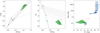 |
Fig. 3. Estimating physical parameters in color-color and color-magnitude space (left and middle panels, respectively) for one example source inside the reddening band. The solid black lines show the pre-main-sequence evolutionary models in the two panels, and the dot-dashed black line shows the canonical CTTS locus of Meyer et al. (1997a) in the color-color diagram. The filled red circles and error bars mark the observed colors and KS magnitude of the source and its photometric errors in the two panels. The dashed red lines show the projection of the observed source toward the models along the appropriate reddening vectors for each panel. These lines intersect the models at the points marked with the blue diamonds in the CC diagram and at the points marked with the orange square in the CMD. The corresponding model points are marked with the same symbols in the two panels, showing that the two estimates do not overlap. The figure also shows the grid of reddened model points (light gray dots) described in Sect. 4. The green areas limit the range of reddened colors and magnitude that provides consistency across all diagrams by allowing for the presence of excess emission (see Sect. 4 for details). Right panel: corresponding ranges of mass and extinction for this example source. For all panels, the models are for an age of 1 Myr and a distance of 1.7 kpc. |
3.2. Color-magnitude diagram
We can similarly use color-magnitude diagrams (CMDs) for independent estimates of extinction and mass, again only for sources without excess emission. If we maintain the assumption that the sources inside the reddening band in a (J − H) vs. (H − Ks) color-color diagram do not have excess emission, their intrinsic colors and magnitudes can be found by dereddening the sources in color-magnitude space to the models, previously shifted vertically by the distance modulus of the cluster. As shown in Fig. 3 (middle panel), the distance between the source (red symbol) and the models along the reddening vector provides a measure for extinction, and the point at which this line intersects the models returns the intrinsic magnitude and color of the source (orange square), hence its mass.
This approach is less likely to produce degenerate masses (and extinctions) than the previous because in color-magnitude space, the models are degenerate for smaller intervals of mass. Still, in Ks vs. (H − Ks) color-magnitude space, for example, models for an age of 1 Myr are degenerate in this sense between ≈2.7 and ≈10 M⊙. This way of estimating the mass depends critically on the knowledge of the distance because the apparent magnitude relates to the absolute magnitude via the distance modulus equation.
We refer to the estimate of extinction and mass in a Ks vs. (H − Ks) color-magnitude diagram as AV, CMD and MCMD, respectively.
3.3. Inconsistency between the CMD and the CC diagram
For the current subset of sources (inside the reddening band), we compared the properties estimated from the KS vs. (H − Ks) CMD with those estimated from the color-color diagram under the assumption that they had no excess. The two estimates should agree if our assumptions were true, but we find that they are consistent only for 269 (37%) out of the 729 sources inside the reddening band, even allowing for photometric errors.
This is illustrated in Fig. 3: the same source dereddens to the blue diamonds in the color-color diagram (left panel) and to the orange square in the color-magnitude diagram (middle panel), corresponding to masses (and luminosities) that are irreconcilable within the errors. If we compare MCC with the mass estimated from J vs. (J − H), which is the combination of color and magnitude that should be least sensitive to excess, we find that the two estimates are still inconsistent for 40% of the sources.
This clearly shows that neither estimate is reliable. It also suggests that our assumptions may be incorrect. We address the possible causes for these inconsistencies in Appendix A.
4. New method: Allowing for excess
In the previous section (Sect. 3), we assumed that the sources inside the reddening band in a (J − H) vs. (H − Ks) color-color diagram did not have excess emission from circumstellar material. This is a common assumption because their colors are consistent with reddened photospheres. We found a strong inconsistency between their properties as estimated in the color-color or in the color-magnitude spaces. It is not unreasonable for these sources to have excess, however: the excess may be small enough for the sources to not cross the red border of the reddening band, and/or some sources may have (small) excess in the flux that is gray and therefore do not alter their colors significantly. If these sources do have excess, then assuming otherwise will naturally produce a discrepancy between the CC and CMD mass estimates because the observed colors and magnitudes in this case are not photospheric. Moreover, the discrepancy will present as a scatter rather than a systematic offset because the excess emission intrinsically depends on many factors.
Because we ruled out other plausible contributions for this inconsistency (cf. Appendix A), we proceed to investigate how allowing for the presence of excess emission impacts the characterization of these sources.
4.1. Defining the parameter space
In the following we assume one distance (1.7 kpc) and one single age (1 Myr) for the cluster. We then attempt to constrain the underlying stellar parameters by finding the range of masses, extinctions, and amounts of excess emission for which the CC diagram and the CMDs produce consistent agreement with the models for each source. We consider that the following assumptions are reasonable:
-
The excess, if it exists, is always red, that is, the observed color of a source cannot be bluer than its photosphere, and the excess eHK in (H − Ks) is always greater than or equal to the excess eJH in (J − H).
-
The colors of the source after removing the excess are bound by the reddening band. This means that the only two phenomena affecting the colors of each source relative to their intrinsic colors are assumed to be the excess emission and extinction.
-
The luminosity produced by the circumstellar material cannot be greater than five times the flux of the source in the Ks band (rK ≤ 5). This is a conservative estimate for sources that are past the protostellar stage for observations in the NIR. According to Eq. (2), this limits the excess in Ks to |eKs| = 1.95 mag (but see Sect. 5.3). For reference, the maximum excess observed in K in Taurus is 1.6 mag (Meyer et al. 1997b).
-
The excess in J must be smaller than or equal to that in H, and the excess in H must be smaller than or equal to that in Ks (|eJ|≤|eH|≤|eKs|). This assumes the spectral energy distribution of the excess emission increases from 1 to 3 μm. Considering the previous assumption, this also limits the excess in J and H to 1.95 mag.
We neglect the contribution of a high accretion luminosity in defining our set of constraints, in particular by assuming that the excess emission is red. This could be relevant for the sources with very high accretion rates, for sources whose accretion flows are exposed, and for sources whose disks are viewed face-on. We expect most of the sources in this subsample to have relatively small disks and low accretion rates already, otherwise they would more likely be found to the right of the reddening band in the CC diagram.
For this particular cluster, Fig. 4 shows that there are barely any sources at extinctions lower than AV ∼ 7 mag, suggesting that the cluster members are located behind a wall of extinction likely created by the part of the cloud that lies in front. We therefore conservatively adopted the additional constraint that the minimum extinction of any cluster member cannot be lower than AV = 5 mag.
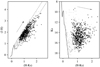 |
Fig. 4. (J − H) vs. (H − Ks) color-color diagram and KS vs. (H − KS) color-magnitude diagram for the observed sources. The black symbols correspond to the sources that are probably cluster members (see Sect. 5.1), and the gray symbols correspond to the remaining sources in the field of view (contaminants). The solid lines in both diagrams represent the adopted models for an age of 1 Myr and a distance of 1.5 kpc. The arrows show the displacement caused by an extinction of 1 mag in KS according to the assumed extinction law (see Sect. 2.1). The dashed lines show the limits of the reddening band in the color-color diagram, defined by the reddening vector and the extreme ends of the model isochrones in color. |
We note that point 3 above is probably too permissive because the colors of a source with a disk corresponding to the maximum allowed excess in KS would most likely appear to the right of the reddening band in a (J − H) vs. (H − Ks) color-color diagram.
We also note that these requirements do not force the existence of excess, they only allow for it if it is necessary to find consistency across color and magnitude space. These constraints and this method therefore answer the question which excess would be required so that the observed colors and fluxes are consistent with the models we adopt for the photospheres of YSOs.
4.2. Method at work
The above conditions, plus the requirement that all observed fluxes and colors must be consistent with the models, constrain the range of intrinsic colors and magnitudes that are plausible for each source, and this then translates into a range of possible combinations of extinction, excess emission, and mass for each source.
In other words, rather than working from the observations to the models, we perform the inverse exercise to search for the combinations within the models that reproduce the observed photometry of each source consistently. To do this, we created a grid of points consisting of the luminosities of the model photospheres reddened by steps of 0.2 mag, then applied the constraints to the grid from the observed colors and magnitudes of each source and their photometric errors, and traced back the allowed ranges of mass, extinction, and excess emission.
Figure 3 illustrates the procedure for one source inside the reddening band. The blue diamonds and the orange square mark the intrinsic colors and KS magnitude expected if the source is dereddened to the models in the CC diagram and in the HK CMD, respectively, assuming no excess emission. For this source, the corresponding mass estimated from the HK CMD is 0.48 M⊙ and that estimated from the CC diagram is either 0.10 or 3.72 M⊙. The right panel uses the same symbols and color codes to illustrate that the corresponding estimates of mass and extinction are irreconcilable when we assume no excess, even allowing for photometric errors.
If we allow for excess emission using the set of constraints defined above (Sect. 4.1), then the green areas show the range of de-excessed colors and KS magnitudes that guarantee that the CC diagram and the CMDs provide consistent estimates for this source, and the green portions of the models show the corresponding ranges of intrinsic colors and magnitudes. This source in particular requires an excess in KS of at least 0.08 mag beyond its photometry uncertainty to produce consistent estimates across the color and magnitude parameter space. Allowing for excess emission, the mass of this source is limited to the range 0.09 − 0.3 M⊙, which is 1.6 to 5 times smaller than the value obtained from the HK CMD assuming no excess.
This example shows that we are exposed to an error that can be large if we do not allow for excess when the masses are derived from photometric data, even for the sources inside the reddening band (see Sect. 5.6.1 for more details). In this case, the interval of possible masses partially overlaps the mass estimate from the CC diagram, but this is not the case for all sources.
The example also shows that the ranges of possible properties for each source are not independent: a fixed extinction, for example, restricts the interval of possible masses (and excess). Furthermore, the properties within these intervals are not equally probable, which means that a Bayesian inference analysis that would incorporate all information available for each source and more realistic expectations for the characteristics of circumstellar material could constrain the properties of each YSO even further. This is beyond the scope of this paper, however. For example, if we consider that the CTTS locus slope of Meyer et al. (1997a) is a good representation of the relation of colors for YSOs with circumstellar material, then the range of properties allowed for the example source in Fig. 3 is limited further to the band defined by the dark green points; the mass of this source then becomes restricted to 0.1 − 0.2 M⊙.
4.3. Sources to the right of the reddening band
The position of sources to the right of the reddening band in the (J − H) vs. (H − Ks) color-color diagram requires that they have excess emission with respect to their photospheres. In addition to extinction, we must therefore determine this excess before we can infer their masses.
For these sources, the standard approach relies on taking the CTTS locus as a single line rather than the direction vector of a continuum of lines whose intercept varies with the spectral type of each source (see Sect. 1). This assumption carries an uncertainty to the extinction that cannot be quantified because the spectral types are not known a priori; although it can be as high as 1 mag in AV according to Meyer et al. (1997a), it is commonly taken to be smaller than the photometric uncertainty and is typically ignored. The procedure is then to deredden all sources that fall within the empirical region of CTTSs in the color-color diagram to the same one line (the CTTS locus; dot-dashed line in Fig. 5) to estimate the extinction of each source. From the extinction, the only way to estimate excess emission and then mass is to assume an excess vector, as mentioned in Sect. 1, in color-magnitude space, but these solutions have not been extensively adopted by the community.
The method we propose to constrain physical parameters, that is, by searching the parameter space for consistency across color and magnitude space, can also be applied to these sources. This is indeed currently the only method that can constrain the mass, extinction, and amount of excess of any individual source from NIR photometry alone, even though it cannot constrain these parameters to a single most probable value, as would be desirable. With other methods, some more or less arbitrary amount of excess must always be assumed to find a value for the mass rather than constraining it from the data.
The selection of sources that fall to the right of the reddening band does not limit the sample to classical T Tauri stars, but includes all sources with excess, that is, Herbig AeBe stars. Our sample contains 94 such sources in total. These sources are redder than reddened photospheres and therefore clearly have excess emission, which activates the condition that their excess must be at least such that their colors have to move to the reddening band in color-color space.
Figure 5 illustrates the procedure for one of these sources. In this case, the mass estimate obtained by dereddening directly to the models in an (H − Ks) vs. KS color-magnitude diagram (marked in the figure by the orange squares) is deliberately incorrect because it is clear from the source position in the color-color diagram that it must have excess, but it is plotted here for completeness. In the left panel, the blue diamond shows where this source would deredden to in the canonical CTTS locus, allowing an estimate of its visual extinction, which would be 7.7 mag in this case. As mentioned above, this value of extinction can be incorrect by more than one magnitude, depending on the actual underlying mass of the object. In the middle panel, we show the position of the source that is dereddened by this amount of extinction (marked by the dot-dashed blue line) in an (H − Ks) vs. KS CMD. It is clear that even if we trusted the extinction calculated using the CTTS locus, we would still lack information to derive the mass of the source because we do not know its excess. Using our method, we constrain the mass of the source to 0.06 to 0.2 M⊙ and infer that its excess in KS must be greater than 0.4 mag.
5. Results
In this section we discuss how this method can distinguish between YSO candidates and background objects, how it can be used to determine the distance to equidistant, coeval populations (e.g., young clusters), and analyze the excess in KS for the sources in RCW 38.
5.1. Membership analysis
The method we propose naturally distinguishes between cluster members and foreground and background sources, making it a very useful tool in evaluating membership. The conditions we impose (see Sect. 4.1) are reasonable for cluster members because they assume a fixed distance and age and allow a set of characteristics for excess emission that is plausible for YSOs. Unrelated sources (or sources with poor photometry) in general do not comply with these conditions, however, either because their distance is different from that of the cluster or because their photometry cannot be reconciled with the models. Therefore, all sources for which the method cannot find a solution were classified as unrelated sources and were eliminated from the cluster sample.
In our dataset, we started with 854 sources. The method found a solution for 705 of these sources. Of these, 123 were below the reddening band, which means that the method cannot find a solution for 2 sources that lie in the CTTS region of the (J − H) vs. (H − Ks) color-color diagram; these are sources that would normally be regarded as cluster members because they display obvious excess emission, but this method suggests they may be contaminants, likely extragalactic. The remaining 582 sources for which the method finds a solution lie inside the reddening band in the (J − H) vs. (H − Ks) color-color diagram.
We find that the solution found for a few sources is unrealistic: they have allowed excess that is very low in color (i.e., the proposed excess is gray in (H − KS)), but high in flux (|emin|> 0.2 mag). This configuration is unlikely for YSOs because excess from circumstellar disks is most often red (|eK|> |eH|), especially when it is high in flux. Conversely, this presentation is expected if the sources have a distance different from what is assumed for the cluster: in this case, the flux in all bands would have the same excess, which would correspond to the difference in distance moduli between the cluster distance and the true distance of the sources. We therefore interpret these sources as background objects and classify them as unrelated as well. In our dataset, we find 69 of these additional sources (68 inside the reddening band and one below the reddening band). This selection does not eliminate all sources with gray excess in (H − KS): those that also have low excess in KS were kept, as it is physically plausible that these sources exist, although we admit some of them may still be contaminants. Its ability to select cluster members means that this method may be useful in identifying targets for follow-up studies, namely for spectroscopic surveys.
After the selection above, our science selection contains 636 cluster members (and 218 unrelated sources), which translates into a membership fraction of 74% (71% if we consider only sources inside the reddening band, as drawn in Fig. A.1 for reference). In the projected area of the field of view, this amounts to a surface density of about 200 YSOs/pc2 (at a distance of 1.5 kpc), although we recall that this dataset is composed of observations using instruments with different resolutions and sensitivities, and the completeness therefore varies across the field of view. Incompleteness precludes the detection of the fainter sources, so that the actual surface density of the cluster is necessarily higher than the value we determine.
Below we assess the reliability of this method in evaluating membership.
5.2. Distance determination
As mentioned in the previous section, the conditions we impose with this method are expected to be reasonable for cluster members provided that the models are correct3 and that the age and distance are correct. Because we know that this sample contains a large number of equidistant and probably coeval sources (the cluster members), the method is expected to result in convergence for the largest number of sources when the correct distance to the population is assumed.
We therefore calculated the number of sources with a solution from the method while varying the assumed distance from 500 to 3500 pc. Figure 6 shows a distribution that has a peak, as expected if an equidistant population is present. The peak is located at 1.5 ± 0.2 kpc, although, considering its width and the statistical error, we cannot rule out distances up to 1.9 kpc. These values agree well with the distance determined independently in other works (see Sect. 1), validating this method as a reliable tool for determining distances to locally dense populations. Although we did not test this in this work, it is foreseeable that this method is most accurate for denser populations without significant age spreads.
 |
Fig. 6. Number of sources for which the photometry can be reconciled with the models in color and magnitude within the photometric errors, assuming an age of 1.0 Myr (solid lines) or 0.5 Myr (dotted lines) for the science sample (black lines, circles) and for the control field (gray lines, squares). The vertical dashed line shows the distance we assume for the cluster (1.5 kpc). |
For comparison, we applied the same procedure to a nearby control field taken from the 2MASS Point Source Catalog (Skrutskie et al. 2006) from a region at the same Galactic latitude as RCW 38, 1.5° West from the cluster in Galactic coordinates. We selected 11 223 sources with good photometry in J, H, and KS and plotted the number of these for which the method found a solution assuming distances in the same range. The results are shown as gray lines in Fig. 6. Although the control field has 13 times more sources than the science field, the method can only find a solution for 50 to 150 sources, and the distribution of this number with an assumed distance does not show any peak.
We can use the control field distribution to estimate how effective the method is at evaluating membership (see Sect. 5.1). Because we know that the control field is unlikely to contain sources from the cluster, we can estimate the number of unrelated sources that the method would erroneously consider cluster members using the criteria defined in Sect. 5.1. Applying a scaling factor to account for the difference in area between the control and the science fields, we estimate that the method would include 0.4 unrelated sources in the science sample. On the other hand, when we apply a scaling factor that accounts for the difference in the number of sources up to KS = 14 mag (the limiting magnitude of the 2MASS sample), we estimate that the method would include 1.3 unrelated sources in the science sample in this magnitude range. The actual difference in sensitivity between the two samples precludes a definitive analysis of the contamination that may still be included in the science sample, but these calculations provide confidence that the method does not include many contaminants in the science sample.
Figure 6 exposes a less obvious feature of this method: In the science sample, the method still finds convergence for many sources when assuming the incorrect distance, whereas in the control field, the method only finds convergence for a residual fraction of the stars. This happens because most of the YSOs in this field need excess to reconcile their photometry with the models. If the assumed distance is not their true distance, then the method may still find a solution because the difference in distance modulus can mimic true excess up to some point. Therefore, it is expected that a sample containing a large number of sources with intrinsic excess presents a higher baseline in Fig. 6 (black lines), as is observed. The numbers in the wings of this distribution are very close to the number of sources for which the method detects excess emission, corroborating that the reason for the much higher numbers in the science sample is the presence of intrinsic excess. The photometry of field stars, on the other hand, is consistent with some model without invoking excess, so that only sources for which a difference in distance modulus can mimic true excess when assuming models for an incorrect age will have a solution, and it is expected that this represents only a residual amount. As explained in Sect. 5.1, the method mitigates for this in a second pass.
This also illustrates that this method cannot be used to estimate distances to individual sources because a given source with excess may still have a solution from the model with an incorrect distance (although the solution will be incorrect). A distance estimate can only be obtained in the way we propose for equidistant and reasonably coeval populations because it relies on the analysis of the group. Consequently, the distance is more significantly constrained for more populous or dense clusters.
In this sense, the effect of photometric incompleteness of the sample is negligible. As long as the sample contains a large enough number of coeval and equidistant sources to warrant sufficient statistics relative to the background and foreground population, the method is expected to be able to determine distances accurately. In the current dataset we estimate that the cluster members represent 74% of all sources detected in J, H, and KS simultaneously, even though the photometric completeness is limited because of the J-band sensitivity (see Sect. 2.2.3).
This method provides a good complement to Gaia (Gaia Collaboration 2018) in determining distances to young clusters. Because they are heavily reddened, these clusters often lack sources visible in the optical (λ < 1 μm), have only too few of these sources to allow for a good handle on the distance to the cluster, or are too distant so that the parallaxes need a higher-order analysis to be converted into distances (Luri et al. 2018). Our method can be used reliably for embedded clusters and to reasonably large distances.
5.3. Distribution of excess
The method we propose calculates the range of excess emission that is required to produce consistent intrinsic colors and magnitudes for each source. The actual amount of excess can be any value within these ranges, and although the excess is not determined with our data, we can characterize the distribution of the minimum excess required.
Figure 7 shows the cumulative distribution of the minimum excess in KS required to fit sources inside the reddening band (514 sources; solid line) and sources to the right of the reddening band (122 sources; dotted line) for which the method finds a solution. As expected, sources inside the reddening band need lower excess on average than sources to the right of the reddening band. In contrast to what is generally assumed, however, this figure shows that sources inside the reddening band also need excess, otherwise their photometry is irreconcilable with the models. For this subset of sources, the figure shows that about 50% need excess higher than the maximum photometric error we allow for in our dataset.
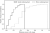 |
Fig. 7. Cumulative distribution of the minimum excess in KS (|eK|) required to find consistent colors and magnitudes for the sources whose colors lie inside the reddening band (solid line) and for those whose colors fall below the reddening band (dotted line). |
Again, these distributions only show the lower limit of the excess emission for these sources, and they therefore do not represent the distribution of actual excess for this cluster, but they do show that the excess distribution is probably not flat.
5.4. Excess fraction of the cluster
The lower limits for the amount of NIR excess for individual sources (see Sect. 5.3) can be used without further assumptions to determine a lower limit for the excess fraction of the cluster. In this way, this method becomes substantially more sensitive than previous methods based on NIR data that select YSOs with excess solely based on their binary position to the left or to the right of the red limit of the reddening band in color-color space.
To account for the effect of photometric errors, we considered only sources that require an excess higher than 0.15 mag in KS (|eK, min|≥0.15). Using this criterion, we find a lower limit for the excess fraction in the Ks band of 57% (364 sources) for RCW 38 in the science sample (see Sect. 5.1). In comparison, only 19% of the sources lie below the reddening band in the (J − H) vs. (H − Ks) color-color diagram. If we vary the distance between 1.3 and 2.0 kpc, and change the age from 1 to 0.5 Myr, we obtain lower limits for the excess fractions between 54% and 59%, confirming a very high excess fraction for this cluster. With the extinction law coefficients from Indebetouw et al. (2005) or from Nishiyama et al. (2009), the excess fraction becomes 59% in both cases for an age of 1 Myr and a distance of 1.5 kpc.
Our estimate is a lower limit because the method returns a range of possible excess for each source and we used the minimum value of these ranges to define a source with excess. For example, if the photometry of a given source can be reconciled with the models by invoking an excess between 0.05 and 0.25 mag, then this source is not included as an excess source in the calculation of the excess fraction, because the lower limit of the range is smaller than the cutoff we defined of 0.15 mag. However, if the true excess of this source were closer to the upper limit of the range, then this source would contribute to increase the excess fraction of the cluster.
The incompleteness of the sample may affect the estimate of the excess fraction of the cluster in the opposite direction. Excess increases the brightness of YSOs by adding flux, which means that if some low-mass YSOs that are not bright enough to be detected by themselves will be detected if they have excess. This may bias the sample toward sources with excess and artificially inflate the excess fraction. However, this is a limited bias because it is not expected that the emission from circumstellar material dominates the total emission of the object in the NIR. Considering that excess is also most likely red, that excess is expected to be prevalent in low-mass YSOs, and that it is the J band that limits the completeness the most (see Fig. 2), we do not expect this effect to bias the results significantly.
Keeping in mind that the minimum excess we refer to is not necessarily the true excess of these sources (they are only lower limits) we searched for a dependence of minimum excess with position within the cluster. This is a frail analysis with this dataset because sensitivity and resolution vary spatially: as described in Sect. 2.2, the inner parts of the cluster were imaged with higher resolution and sensitivity than the outer parts, and these differences in completeness can influence the detection of excess. With this in mind, we do not find that the sources that require the highest excess avoid the proximity to the O-binary. This may suggest that the massive stars have not (yet?) had a significant impact on the K-band excess from the inner disk, or that dynamics was already efficient in relocating stars from the place where their disks were affected.
The excess fraction we derive is comparable to the fraction found using MIR data with X-ray membership analysis for the same cluster (70%, although over a larger projected area and using lower-resolution data; Winston et al. 2011). The gold standard for detecting circumstellar material through excess emission is using MIR observations, but this analysis suggests that this method may be comparably sensitive, with the caveat that the near- and MIR probe different regions and different properties of the disk. This is a significant advance in the study of young clusters because it opens the opportunity to analyze the presence of disks in more challenging populations: current NIR instrumentation delivers spatial resolutions that are several times better than in the MIR. This allows studies of more distant clusters and of clusters with higher stellar densities with an accuracy that is comparable to that of studies of nearby, less massive and less dense environments, namely by mitigating the effects of blended (unresolved) sources that can easily inflate the number of excess sources artificially. Moreover, NIR emission is still largely dominated by the object photosphere, whereas the MIR is more sensitive to the emission from the disks. NIR observations are therefore less likely to be biased toward the detection of sources with disks, which would artificially enhance excess fractions. Finally, NIR observations are easily obtained using ground-based telescopes and straightforward techniques, whereas MIR data require space-based observations or expensive (in telescope time) ground-based observations and sophisticated techniques to achieve comparable performance because the sky is too bright in these wavelengths.
5.5. Effect of unresolved binaries
We have tested the method for the presence of unresolved binaries using artificial star experiments. Any estimate of YSO parameters (mass, excess and extinction) is incorrect for unresolved binaries if the method provides a solution that is based on the expected parameters for single sources, as the present method does. However, because it provides only lower and upper limits, the tests show that these limits still encompass the mass and extinction of the binary.
The method was able to identify the vast majority of (cluster) YSOs from background objects, both unresolved binaries and single sources, in the artificial data. The method proved effective in finding the correct distance in the artificial data, that is, in the presence of unresolved binaries. The excess fraction changes when unresolved binaries are included, although it remains underestimated. In other words, the method still accurately predicts a reliable lower limit for the fraction of excess sources in the cluster, even in the presence of unresolved binaries, and even if the excess fraction is as high as 100%.
The reason for this is that the combined magnitude and colors of two blended sources with the same extinction (cluster members) is not too different from those of each component, and the method can nevertheless detect the excess. These conclusions hold as long as the blending is not severe; if one detected source corresponds to many YSOs due to a combination of poor resolution and large distance, then more YSOs will be discarded from the sample, which may impact the estimate of the excess fraction of the cluster, for example.
We therefore conclude that the method is robust against unresolved binaries in determining global cluster parameters (distance and excess fraction) and in detecting most cluster members if the blending is not severe.
5.6. Constraining masses
This method provides constraints for the mass of YSOs, as it does for excess, as we illustrated in Sect. 4.2. The method returns an interval of plausible masses for each source, and not a single most likely value, as would be desirable.
Our results suggest that the upper limit of the mass interval estimated for each source is likely an overestimate because it most often corresponds to no excess in both J and H (and to the least amount of excess in KS). Although this is allowed by the conditions we defined, most sources have a minimum excess in KS higher than 0.1 mag, which means that the emitted flux in KS of the circumstellar disk is more than 10% of the flux emitted by the YSO itself. If a YSO still has such a substantial disk, it is also likely to still have a measurable excess (at least) in H (see also Furlan et al. 2011). This means that if we were to impose some correlation between the excess in KS and in H, then the upper limit for the mass of most sources would be lower. If we adopt the slope of Meyer et al. (1997a) as the relation between color excess in (J − H) and (H − KS), then the upper limits for the mass ranges allowed are lower than if we do not impose any relation between the color of the excess emission, although we find that this relation is not suitable for all objects in the sample.
The results provided by this method can unfortunately not be used to reasonably constrain the mass function (MF) of the cluster because the allowed mass intervals for each source are too wide to allow a meaningful constraint. This method might at most be used to rule out some extreme forms of the MF by sampling the allowed intervals for individual sources a large enough number of times using Monte Carlo methods and statistics. This was not attempted in this work.
5.6.1. Consequences of neglecting excess emission
Figure 8 shows the comparison between the masses estimated using the KS vs. (H − Ks) CMD assuming they do not have excess emission and ignoring the inconsistency they present with the colors in the CC diagram and those estimated using the method we propose for the sources inside the reddening band. The vertical gray bands represent the range of allowed masses for each source, that is, the masses corresponding to the green areas in Fig. 3. As expected, compared to when we allow sources to have excess, the CMD typically overestimates the mass, in many cases by more than 100% even for this subsample of sources (sources inside the reddening band), because the excess emission is taken as photospheric flux. The inverted triangles show the mass that corresponds to the least amount of KS-band excess emission, which typically corresponds to the upper limit of the allowed mass range for each source. Figure 9 shows a cumulative histogram of the ratio of the mass estimated directly from the CMD and the mass corresponding to the least excess (inverted triangles in Fig. 8); this ratio corresponds to the minimum relative error in the mass of a source if we take the mass from the CMD assuming no excess emission. The figure shows, for example, that for 40% of the sources, the CMD overestimates the mass by at least 1.5 times relative to their allowed masses.
 |
Fig. 8. Comparison between the masses estimated by the new method, allowing excess emission (allowed masses; Sect. 5.6.1) and the masses inferred from the KS vs. (H − Ks) CMD (MCMD) assuming no excess emission. The vertical gray bands represent the range of allowed masses for each source, and the inverted triangles highlight the mass in this interval that corresponds to the least amount of excess emission. The horizontal error bar reflects the uncertainty in mass from photometric errors, except for the points inside the area delimited by the dashed lines, which corresponds to the range of masses in which the models are degenerate: in this area, the horizontal error bars encompass the minimum and maximum possible values from the models. The dashed red line is the identity line. |
 |
Fig. 9. Cumulative histogram of the ratio of the mass estimated directly from the CMD and the mass corresponding to the least excess for the sources inside the reddening band. This is a measure of the minimum factor by which the mass may be overestimated from the CMD. |
5.6.2. Using the J vs. (J − H) CMD to narrow down masses
The right panel of Fig. 3 also shows the mass and extinction estimates from a J vs. (J − H) CMD within the photometric errors (filled yellow squares) for the example source. Based on the typical spectral energy distribution of the excess emission and our assumptions in particular, this band and this color should be the least affected by excess emission. As long as the excess is low, this color-magnitude space therefore is the most likely to provide the correct estimate for the mass of each source. Figure 3 shows that the mass and extinction estimates from this color-magnitude space for one example source overlap the range of allowed masses derived in Sect. 4 for almost all sources (84%). Unsurprisingly, they overlap the estimates that correspond to the least amount of KS-band excess emission. The question is whether this means that dereddening the sources to the models in the J vs. (J − H) CMD provides the correct mass, at least for the sources inside the reddening band. This is not necessarily the case.
As we described in the previous section, the upper limit of the mass estimate for each source is likely an overestimate of the true mass. Furthermore, the estimate from the J vs. (J − H) CMD is still inconsistent with the estimate from the (J − H) vs. (H − Ks) color-color diagram (yellow vs. blue points in the right panel Fig. 3). This can only happen if there is excess exclusively in KS, that is, if the excess in J and in H is zero: in this case, the (H − KS) color in the CC diagram would be offset from the reddened photospheric color, but the (J − H) color would be correct, as would the J-band magnitude. Although this is plausible for sources with low excess in KS because the excess in H and in J would then be even lower, it becomes unlikely for sources with relatively high KS-band excess. In Sect. 5.3 we showed that a significant fraction of sources indeed require such KS-band excess, suggesting that the excess at least in H is also likely to be measurable, which in turn suggests that the J − (J − H) CMD cannot typically estimate the mass correctly. Rather, this ubiquitous overlap of the J − (J − H) mass estimate and the range of allowed masses is an expected consequence of the constraints we assumed (Sect. 4.1) because we allow the possibility of having excess only in KS. We can at best say that the J − (J − H) CMD provides a still unlikely upper limit for the mass of the sources that lie inside the reddening band.
5.7. Applicability to other star-forming regions
This analysis was conducted using data for one specific region, RCW 38. This method can be applied to any NIR dataset of YSOs containing J-, H-, and K-band photometry, however.
The method we propose does not introduce any new principle; we suggest that the photometric information from the three bands J, H, and K for a given source should be used consistently, along with the theoretical models, instead of using preferentially one photometric band and/or color. In this sense, the dataset for RCW 38 is only an example of how this can be done and an example for the use of NIR photometry to characterize clusters.
As mentioned before, this method only allows determining distances to equidistant and reasonably coeval populations. Since it relies on the statistical significance of the number of cluster members in the dataset, the distance is more significantly constrained the more populous the population.
The realization that the mass estimates from several color and magnitude combinations are inconsistent with each other is independent of the targeted region. RCW 38 is a very young cluster, therefore the probability of its sources having disks is higher than for older clusters, and these results may therefore be more evident for this region than they would be for an older population. They showed that it is not reasonable to assume a priori that sources inside the reddening band do not have excess, however, and that this assumption may lead to large errors in the estimate of mass, for example. If the sources do not have excess, then this method will show that the colors and fluxes are consistent with each other without having to invoke the presence of disks.
One limitation of the method we propose is the necessity of J-band photometry because this is the band that is most affected by interstellar extinction. For high extinction values (and large distances), the lowest-mass YSOs cannot be detected in J with reasonable observing times. This problem will be mitigated with the advent of 30-meter-class telescopes, whose collecting power will be substantially larger, but this will always remain a limitation of this method. Still, compared to the limitations inherent to other methods for determining distances, memberships, and excess fractions, and considering that the alternative of using only the more sensitive H and/or K bands may produce flawed results (cf. Sect. 5.6.1), we accept this limitation as necessary.
Like all other methods, this method relies on data with adequate spatial resolution. An inadequate combination of large distance, high stellar density, and poor spatial resolution will cause cluster members to be blended with other cluster members or with unrelated sources. In both cases, the estimates for the individual properties will be off, as with any other method that cannot distinguish the two objects. As mentioned in Sect. 5.5, the method is robust against unresolved binaries, but it cannot accommodate many blended YSOs or blended sources consisting of YSOs and unrelated objects with very different extinctions. In this case, the combined photometry will be too disparate for the method to be able to converge for that source, and it will be discarded from the cluster sample. This will affect membership determination, and also the estimates for distance and excess fraction. This method is therefore not appropriate for observations of clusters with inadequate resolutions relative to their distance and surface density.
We also caution that the sensitivity of the method to detecting YSOs (cluster members) likely decreases as a function of cluster age; the photometric properties of older YSOs are progressively more similar to those of main-sequence stars, so that the method will converge more easily for unrelated objects if it expects the YSOs to have photometry that is not too different from field stars.
We recommend these results to be taken into account at the observing proposal stage for other regions, such that datasets used for the study of young clusters include all three standard photometric broad bands J, H, and K with adequate exposure times. This calls for comparatively longer observations in J, and with adequate spatial resolution.
6. Conclusions
Our study showed that NIR data can be very powerful in analyzing young stellar clusters, more so than they are usually given credit for. The main conclusions of this paper are listed below.
-
We propose a new method that uses information from J, H, and KS bands simultaneously to determine the distance to a cluster, assess the membership of individual sources, determine the fraction of sources that have excess emission from the hot inner rim of the circumstellar disks, and constrain the masses, NIR excess, and foreground extinction of individual YSOs independently of other observations.
-
The method returns a lower limit to the fraction of sources with excess in the cluster that is comparable to the fraction derived from existing MIR surveys, but at a higher resolution. This new opportunity can be a powerful tool for understanding the impact of massive stars and cluster environments on the evolution of circumstellar material across the Milky Way. For RCW 38, we find a lower limit for the excess fraction in the Ks band of ≈60%.
-
We find that masses derived from NIR colors and magnitudes can be substantially overestimated using procedures that do not take the information from the three photometric bands into account. This happens when sources whose colors fall inside the reddening band in a color-color diagram are (incorrectly) assumed to have no excess emission. The method we propose can constrain the range of possible mass and excess emission for single sources, both those whose colors lie inside and those that lie below the reddening band in a (J − H) vs. (H − Ks) color-color diagram.
-
These results affect studies of individual sources and population studies, in particular studies of the initial mass function (IMF) in young and embedded clusters, which naturally rely on an accurate handle on individual masses. The bias is stronger at the low end of the mass spectrum, where most IMF research of embedded clusters is currently focused.
-
The method presented here bodes well for future studies of young clusters across the Milky Way. The upcoming generation of ground-based telescopes, such as the ELT, will have NIR instrumentation that is suited to constrain distances and memberships of deeply embedded or obscured young cluster across the entire Galactic plane.
Although these results are drawn from the analysis of one single cluster, the procedure is general and can be applied to any catalog of YSOs with photometry in J, H, and K, provided the sources are reasonably coeval and equidistant. The gain in using this procedure with respect to estimating masses directly from a single-band luminosity or from a single combination of color and magnitude without accounting for excess is greater for younger populations because circumstellar material tends to dissipate over time.
Acknowledgments
This work had the financial support of FCT, Portugal (grant ref. SFRH/BPD/101562/2014 and FCT contract number UIDB/00099/2020). A warm thanks to J. Alves for very useful discussions that brought clarity to this work. Thank you also to P. Garcia for suggestions, and to the referee, Prof. Sebastian Ramirez Alegria, whose thoughtful comments contributed to improve the paper. Based on observations collected at the European Southern Observatory under ESO programmes 70.C-0400(A), 70.C-0729(A), and 074.C-0728(A).
References
- Adams, F. C., Hollenbach, D., Laughlin, G., & Gorti, U. 2004, ApJ, 611, 360 [NASA ADS] [CrossRef] [Google Scholar]
- Ansdell, M., Williams, J. P., Manara, C. F., et al. 2017, AJ, 153, 240 [Google Scholar]
- Armitage, P. J., & Hansen, B. M. S. 1999, Nature, 402, 633 [NASA ADS] [CrossRef] [Google Scholar]
- Ascenso, J., Alves, J., Beletsky, Y., & Lago, M. T. V. T. 2007a, A&A, 466, 137 [NASA ADS] [CrossRef] [EDP Sciences] [Google Scholar]
- Ascenso, J., Alves, J., Vicente, S., & Lago, M. T. V. T. 2007b, A&A, 476, 199 [NASA ADS] [CrossRef] [EDP Sciences] [Google Scholar]
- Avedisova, V. S., & Palous, J. 1989, Bull. Astron. Inst. Czechoslov., 40, 42 [Google Scholar]
- Balog, Z., Muzerolle, J., Rieke, G. H., et al. 2007, ApJ, 660, 1532 [NASA ADS] [CrossRef] [Google Scholar]
- Baraffe, I., Homeier, D., Allard, F., & Chabrier, G. 2015, A&A, 577, A42 [NASA ADS] [CrossRef] [EDP Sciences] [Google Scholar]
- Barentsen, G., Vink, J. S., Drew, J. E., et al. 2011, MNRAS, 415, 103 [CrossRef] [Google Scholar]
- Beltrán, M. T., & de Wit, W. J. 2016, A&ARv, 24, 6 [Google Scholar]
- Bertin, E. 2006, in Astronomical Data Analysis Software and Systems XV, eds. C. Gabriel, C. Arviset, D. Ponz, & S. Enrique, ASP Conf. Ser., 351, 112 [Google Scholar]
- Bertin, E., Mellier, Y., Radovich, M., et al. 2002, in Astronomical Data Analysis Software and Systems XI, eds. D. A. Bohlender, D. Durand, & T. H. Handley, ASP Conf. Ser., 281, 228 [NASA ADS] [Google Scholar]
- Bressan, A., Marigo, P., Girardi, L., et al. 2012, MNRAS, 427, 127 [NASA ADS] [CrossRef] [Google Scholar]
- Cardelli, J. A., Clayton, G. C., & Mathis, J. S. 1989, ApJ, 345, 245 [Google Scholar]
- Carpenter, J. M. 2001, AJ, 121, 2851 [Google Scholar]
- Comerón, F., & Schneider, N. 2007, A&A, 473, 149 [NASA ADS] [CrossRef] [EDP Sciences] [Google Scholar]
- Concha-Ramírez, F., Portegies Zwart, S., & Wilhelm, M. J. C. 2022, MNRAS, submitted [arXiv:2101.07826] [Google Scholar]
- D’Alessio, P., Cantö, J., Calvet, N., & Lizano, S. 1998, ApJ, 500, 411 [Google Scholar]
- D’Alessio, P., Calvet, N., Hartmann, L., Lizano, S., & Cantó, J. 1999, ApJ, 527, 893 [CrossRef] [Google Scholar]
- D’Alessio, P., Calvet, N., & Hartmann, L. 2001, ApJ, 553, 321 [Google Scholar]
- Damiani, F., Micela, G., & Sciortino, S. 2016, A&A, 596, A82 [NASA ADS] [CrossRef] [EDP Sciences] [Google Scholar]
- DeRose, K. L., Bourke, T. L., Gutermuth, R. A., et al. 2009, AJ, 138, 33 [CrossRef] [Google Scholar]
- Devillard, N. 1997, The Messenger, 87, 19 [NASA ADS] [Google Scholar]
- Drake, J. J., Ercolano, B., Flaccomio, E., & Micela, G. 2009, ApJ, 699, L35 [NASA ADS] [CrossRef] [Google Scholar]
- Drass, H., Haas, M., Chini, R., et al. 2016, MNRAS, 461, 1734 [NASA ADS] [CrossRef] [Google Scholar]
- Facchini, S., Clarke, C. J., & Bisbas, T. G. 2016, MNRAS, 457, 3593 [NASA ADS] [CrossRef] [Google Scholar]
- Fang, M., van Boekel, R., King, R. R., et al. 2012, A&A, 539, A119 [NASA ADS] [CrossRef] [EDP Sciences] [Google Scholar]
- Frogel, J. A., & Persson, S. E. 1974, ApJ, 192, 351 [NASA ADS] [CrossRef] [Google Scholar]
- Furlan, E., Luhman, K. L., Espaillat, C., et al. 2011, ApJS, 195, 3 [Google Scholar]
- Gaia Collaboration (Brown, A. G. A., et al.) 2018, A&A, 616, A1 [NASA ADS] [CrossRef] [EDP Sciences] [Google Scholar]
- Getman, K. V., Feigelson, E. D., Kuhn, M. A., et al. 2014, ApJ, 787, 108 [Google Scholar]
- Gillespie, A. R., White, G. J., & Watt, G. D. 1979, MNRAS, 186, 383 [CrossRef] [Google Scholar]
- González-Fernández, C., Asensio Ramos, A., Garzón, F., Cabrera-Lavers, A., & Hammersley, P. L. 2014, ApJ, 782, 86 [CrossRef] [Google Scholar]
- Guarcello, M. G., Prisinzano, L., Micela, G., et al. 2007, A&A, 462, 245 [NASA ADS] [CrossRef] [EDP Sciences] [Google Scholar]
- Guarcello, M. G., Micela, G., Damiani, F., et al. 2009, A&A, 496, 453 [NASA ADS] [CrossRef] [EDP Sciences] [Google Scholar]
- Guarcello, M. G., Micela, G., Peres, G., Prisinzano, L., & Sciortino, S. 2010, A&A, 521, A61 [CrossRef] [EDP Sciences] [Google Scholar]
- Habibi, M., Stolte, A., Brandner, W., Hußmann, B., & Motohara, K. 2013, A&A, 556, A26 [NASA ADS] [CrossRef] [EDP Sciences] [Google Scholar]
- Harayama, Y., Eisenhauer, F., & Martins, F. 2008, ApJ, 675, 1319 [Google Scholar]
- Haworth, T. J., Facchini, S., Clarke, C. J., & Mohanty, S. 2018, MNRAS, 475, 5460 [NASA ADS] [CrossRef] [Google Scholar]
- Hillenbrand, L. A., & Carpenter, J. M. 2000, ApJ, 540, 236 [NASA ADS] [CrossRef] [Google Scholar]
- Indebetouw, R., Mathis, J. S., Babler, B. L., et al. 2005, ApJ, 619, 931 [NASA ADS] [CrossRef] [Google Scholar]
- Johnstone, D., Hollenbach, D., & Bally, J. 1998, ApJ, 499, 758 [NASA ADS] [CrossRef] [Google Scholar]
- Lada, C. J. 1987, in Star Forming Regions, eds. M. Peimbert, & J. Jugaku, IAU Symp., 115, 1 [NASA ADS] [Google Scholar]
- Lada, C. J., & Adams, F. C. 1992, ApJ, 393, 278 [Google Scholar]
- Lada, C. J., Muench, A. A., Luhman, K. L., et al. 2006, AJ, 131, 1574 [Google Scholar]
- Lenzen, R., Hartung, M., Brandner, W., et al. 2003, in Instrument Design and Performance for Optical/Infrared Ground-based Telescopes, eds. M. Iye, & A. F. M. Moorwood, Proc. SPIE, 4841, 944 [NASA ADS] [CrossRef] [Google Scholar]
- López-Chico, T., & Salas, L. 2007, Rev. Mex. Astron. Astrofis., 43, 155 [NASA ADS] [Google Scholar]
- Luri, X., Brown, A. G. A., Sarro, L. M., et al. 2018, A&A, 616, A9 [NASA ADS] [CrossRef] [EDP Sciences] [Google Scholar]
- Mann, R. K., Di Francesco, J., Johnstone, D., et al. 2014, ApJ, 784, 82 [NASA ADS] [CrossRef] [Google Scholar]
- Mesa-Delgado, A., Zapata, L., Henney, W. J., Puzia, T. H., & Tsamis, Y. G. 2016, ApJ, 825, L16 [NASA ADS] [CrossRef] [Google Scholar]
- Meyer, M. R., Calvet, N., & Hillenbrand, L. A. 1997a, AJ, 114, 288 [Google Scholar]
- Meyer, M. R., Beckwith, S. V. W., & Natta, A. 1997b, in Herbig-Haro Flows and the Birth of Stars, eds. B. Reipurth, & C. Bertout, IAU Symp., 182, 224P [NASA ADS] [Google Scholar]
- Moorwood, A., Cuby, J. G., & Lidman, C. 1998a, The Messenger, 91, 9 [Google Scholar]
- Moorwood, A., Cuby, J. G., Biereichel, P., et al. 1998b, The Messenger, 94, 7 [NASA ADS] [Google Scholar]
- Muench, A. A., Lada, E. A., Lada, C. J., & Alves, J. 2002, ApJ, 573, 366 [NASA ADS] [CrossRef] [Google Scholar]
- Mužić, K., Schödel, R., Scholz, A., et al. 2017, MNRAS, 471, 3699 [CrossRef] [Google Scholar]
- Muzzio, J. C. 1979, AJ, 84, 639 [NASA ADS] [CrossRef] [Google Scholar]
- Neichel, B., Samal, M. R., Plana, H., et al. 2015, A&A, 576, A110 [NASA ADS] [CrossRef] [EDP Sciences] [Google Scholar]
- Nishiyama, S., Tamura, M., Hatano, H., et al. 2009, ApJ, 696, 1407 [NASA ADS] [CrossRef] [Google Scholar]
- Owen, J. E., Ercolano, B., & Clarke, C. J. 2011, MNRAS, 412, 13 [Google Scholar]
- Preibisch, T., Hodgkin, S., Irwin, M., et al. 2011, ApJS, 194, 10 [Google Scholar]
- Radhakrishnan, V., Goss, W. M., Murray, J. D., & Brooks, J. W. 1972, ApJS, 24, 49 [NASA ADS] [CrossRef] [Google Scholar]
- Richert, A. J. W., Feigelson, E. D., Getman, K. V., & Kuhn, M. A. 2015, ApJ, 811, 10 [NASA ADS] [CrossRef] [Google Scholar]
- Rieke, G. H., & Lebofsky, M. J. 1985, ApJ, 288, 618 [Google Scholar]
- Roccatagliata, V., Bouwman, J., Henning, T., et al. 2011, ApJ, 733, 113 [NASA ADS] [CrossRef] [Google Scholar]
- Rochau, B., Brandner, W., Stolte, A., et al. 2011, MNRAS, 418, 949 [NASA ADS] [CrossRef] [Google Scholar]
- Rousset, G., Lacombe, F., Puget, P., et al. 2003, in Adaptive Optical System Technologies II, eds. P. L. Wizinowich, & D. Bonaccini, Proc. SPIE, 4839, 140 [Google Scholar]
- Scholz, A., Geers, V., Clark, P., Jayawardhana, R., & Muzic, K. 2013, ApJ, 775, 138 [NASA ADS] [CrossRef] [Google Scholar]
- Sellek, A. D., Booth, R. A., & Clarke, C. J. 2020, MNRAS, 492, 1279 [NASA ADS] [CrossRef] [Google Scholar]
- Skrutskie, M. F., Cutri, R. M., Stiening, R., et al. 2006, AJ, 131, 1163 [NASA ADS] [CrossRef] [Google Scholar]
- Stolte, A., Brandner, W., Brandl, B., & Zinnecker, H. 2006, AJ, 132, 253 [NASA ADS] [CrossRef] [Google Scholar]
- Stolte, A., Morris, M. R., Ghez, A. M., et al. 2010, ApJ, 718, 810 [NASA ADS] [CrossRef] [Google Scholar]
- Tody, D. 1986, in Instrumentation in Astronomy VI, ed. D. L. Crawford, SPIE Conf. Ser., 627, 733 [NASA ADS] [CrossRef] [Google Scholar]
- Tody, D. 1993, in Astronomical Data Analysis Software and Systems II, eds. R. J. Hanisch, R. J. V. Brissenden, & J. Barnes, ASP Conf. Ser., 52, 173 [Google Scholar]
- Williams, J. P., & Cieza, L. A. 2011, ARA&A, 49, 67 [Google Scholar]
- Winston, E., Wolk, S. J., Bourke, T. L., et al. 2011, ApJ, 743, 166 [NASA ADS] [CrossRef] [Google Scholar]
- Wolk, S. J., Spitzbart, B. D., Bourke, T. L., & Alves, J. 2006, AJ, 132, 1100 [NASA ADS] [CrossRef] [Google Scholar]
Appendix A: Understanding the inconsistency between the CMD and the CC diagram
In this section, we explore the possible causes for the inconsistency found in the parameters estimated from the CMD and the CC diagram (Sect. 3) for the sources inside the reddening band. We argue that this inconsistency is not likely related with sample contamination, or with assuming an incorrect age or distance for the cluster.
A.1. Effect of sample contamination
One explanation for the inconsistency between the CC and CMD estimates could be that the sample is dominated by unrelated sources: unlike cluster members, field stars are distributed over a range of distances and have a range of ages, so that estimating their mass from one single stellar evolution isochrone at a fixed distance would result in a similar inconsistency, at least qualitatively.
According to the calculations in Sect. A, the colors and magnitudes of only 16% of the sources in our field of view are consistent with the models, therefore only they might be cluster members if this were the correct explanation. If we include the 94 sources that lie to the right of the reddening band as cluster members as well because these sources must have excess and therefore must be young, the sample would still only contain 27% cluster members. In this scenario, we would have a contamination of 73% in this field. This sample in particular is very unlikely to be so severely contaminated by unrelated sources: the field of view is very narrow, and it is centered on a cluster that is rich and dense and that is deeply embedded in a molecular cloud. The molecular cloud creates a wall of extinction, especially in the J band, which naturally filters many background contaminants. For these reasons, we instead expect that most of the observed sources are cluster members. It is accordingly not reasonable to accept such a high contamination fraction. We therefore rule out that the main cause for the observed inconsistency between MCC and MCMD is contamination of the sample from unrelated objects.
A.2. Effect of distance
An incorrect distance might explain the discrepancy between the estimates of mass and luminosity from the CMD and the CC diagram. Altering the assumed distance does not change the estimate from the CC diagram, but shifts the models in magnitude in the CMD, producing different estimates from the CMD.
We investigated whether changing only the assumed distance (while keeping the assumption that these sources do not have excess emission) would increase the fraction of sources for which both colors and magnitudes are consistent with the models and our current assumptions. Figure A.1 shows that this fraction does not change significantly when the distance varies from 500 to 3500 pc: if an incorrect distance were the dominant cause for the discrepancy, then this fraction would have a clear peak at the correct distance because many sources (the cluster members) are expected to lie at the same distance. Instead, the variations are within the expected uncertainties from pure number statistics, and the fraction never rises above 20%. It is also implausible that these many YSOs are spread over a wide range of distances because they are deeply embedded in the molecular cloud. We therefore rule out that the observed inconsistency between colors and magnitudes is due to an incorrect distance.
 |
Fig. A.1. Fraction of sources inside the reddening band for which the photometry can be reconciled with the models in color and magnitude within the photometric errors, assuming an age of 1.0 Myr (solid line) or 0.5 Myr (dotted line). For reference, the dashed line shows the fraction of sources that we estimate are cluster members in Sect. 5.1. |
A.3. Effect of age
An incorrect age for the cluster might also cause a mismatch between the CC and CMD mass estimates. There are several independent indications that RCW 38 is a very young cluster (see Sect. 1), in particular younger than 1 Myr. We therefore analyzed how changing the model isochrone (i.e., the expected intrinsic colors and magnitudes as a function of mass) from 1 to 0.5 Myr would alter the fraction of sources for which the CC and CMD mass estimates agree, while varying the distance as before.
We find that changing the assumed age changes the distribution for all distances, but the values remain similar (Fig. A.1, dashed line). In particular, there is also no distance for which more than 20% of the sources agree between the CC and the CMD using the 0.5 Myr isochrone. We therefore conclude that the observed inconsistency between colors and magnitudes is not due to assuming an incorrect age for the cluster either.
This confirmation was made assuming a single-age population. We therefore cannot formally rule out the possibility that an age spread might explain the inconsistency between the CC and CMD mass estimates. However, there is no evidence in the literature that this cluster has a significant age spread. Its deeply embedded state and its compact morphology, added to the fact that we do not probe too far off the center of the cluster with these data, argue against that for this dataset.
All Tables
All Figures
|
Fig. 1. JHKs color-composite of RCW38 imaged with the SOFI instrument, which has a wider field of view in our dataset. Equatorial north is up and east is to the left; red is Ks, green is H, and blue is J. The field of view covers 4.1′×3.9′ in longitude and latitude (1.8 × 1.7 pc at a distance of 1.5 kpc). |
| In the text | |
|
Fig. 2. Distribution of the apparent brightness of all observed sources (dotted histograms) and of the sources detected concurrently in J, H, and KS (final sample; hatched histograms). |
| In the text | |
|
Fig. 3. Estimating physical parameters in color-color and color-magnitude space (left and middle panels, respectively) for one example source inside the reddening band. The solid black lines show the pre-main-sequence evolutionary models in the two panels, and the dot-dashed black line shows the canonical CTTS locus of Meyer et al. (1997a) in the color-color diagram. The filled red circles and error bars mark the observed colors and KS magnitude of the source and its photometric errors in the two panels. The dashed red lines show the projection of the observed source toward the models along the appropriate reddening vectors for each panel. These lines intersect the models at the points marked with the blue diamonds in the CC diagram and at the points marked with the orange square in the CMD. The corresponding model points are marked with the same symbols in the two panels, showing that the two estimates do not overlap. The figure also shows the grid of reddened model points (light gray dots) described in Sect. 4. The green areas limit the range of reddened colors and magnitude that provides consistency across all diagrams by allowing for the presence of excess emission (see Sect. 4 for details). Right panel: corresponding ranges of mass and extinction for this example source. For all panels, the models are for an age of 1 Myr and a distance of 1.7 kpc. |
| In the text | |
|
Fig. 4. (J − H) vs. (H − Ks) color-color diagram and KS vs. (H − KS) color-magnitude diagram for the observed sources. The black symbols correspond to the sources that are probably cluster members (see Sect. 5.1), and the gray symbols correspond to the remaining sources in the field of view (contaminants). The solid lines in both diagrams represent the adopted models for an age of 1 Myr and a distance of 1.5 kpc. The arrows show the displacement caused by an extinction of 1 mag in KS according to the assumed extinction law (see Sect. 2.1). The dashed lines show the limits of the reddening band in the color-color diagram, defined by the reddening vector and the extreme ends of the model isochrones in color. |
| In the text | |
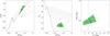 |
Fig. 5. Same as Fig. 3, but for an example source to the right of the reddening band. |
| In the text | |
|
Fig. 6. Number of sources for which the photometry can be reconciled with the models in color and magnitude within the photometric errors, assuming an age of 1.0 Myr (solid lines) or 0.5 Myr (dotted lines) for the science sample (black lines, circles) and for the control field (gray lines, squares). The vertical dashed line shows the distance we assume for the cluster (1.5 kpc). |
| In the text | |
|
Fig. 7. Cumulative distribution of the minimum excess in KS (|eK|) required to find consistent colors and magnitudes for the sources whose colors lie inside the reddening band (solid line) and for those whose colors fall below the reddening band (dotted line). |
| In the text | |
|
Fig. 8. Comparison between the masses estimated by the new method, allowing excess emission (allowed masses; Sect. 5.6.1) and the masses inferred from the KS vs. (H − Ks) CMD (MCMD) assuming no excess emission. The vertical gray bands represent the range of allowed masses for each source, and the inverted triangles highlight the mass in this interval that corresponds to the least amount of excess emission. The horizontal error bar reflects the uncertainty in mass from photometric errors, except for the points inside the area delimited by the dashed lines, which corresponds to the range of masses in which the models are degenerate: in this area, the horizontal error bars encompass the minimum and maximum possible values from the models. The dashed red line is the identity line. |
| In the text | |
|
Fig. 9. Cumulative histogram of the ratio of the mass estimated directly from the CMD and the mass corresponding to the least excess for the sources inside the reddening band. This is a measure of the minimum factor by which the mass may be overestimated from the CMD. |
| In the text | |
|
Fig. A.1. Fraction of sources inside the reddening band for which the photometry can be reconciled with the models in color and magnitude within the photometric errors, assuming an age of 1.0 Myr (solid line) or 0.5 Myr (dotted line). For reference, the dashed line shows the fraction of sources that we estimate are cluster members in Sect. 5.1. |
| In the text | |
Current usage metrics show cumulative count of Article Views (full-text article views including HTML views, PDF and ePub downloads, according to the available data) and Abstracts Views on Vision4Press platform.
Data correspond to usage on the plateform after 2015. The current usage metrics is available 48-96 hours after online publication and is updated daily on week days.
Initial download of the metrics may take a while.