© ESO 2022

1. Introduction

Two-point statistics of the cosmic density field are the principal tools for constraining cosmological models. Large-scale galaxy surveys, such as the Sloan Digital Sky Survey (Tegmark et al. 2004), 2MASS (Allgood et al. 2001), APM Galaxy Survey-2 (Baugh & Efstathiou 1994), 2dF (Percival et al. 2001), BOSS (Dawson et al. 2013), DESI (DESI Collaboration 2016), Pan-STARRS (Chambers et al. 2016), or the DES (The Dark Energy Survey Collaboration 2005), provide data for such measurements. Even larger surveys are planned for the near future, for example Euclid (Tutusaus et al. 2020), WFIRST/Roman (Green et al. 2012), SPHEREx (Doré et al. 2014), LSST/Rubin (LSST Science Collaboration 2009), and the Subaru Prime-Focus Spectrograph (Tamura et al. 2016). While some day we might map the cosmological density field of the observable Universe, at present these wide field surveys are complemented with narrower deep surveys, such as COSMOS (Scoville et al. 2007) and H20 (Beck et al. 2020), the deep survey mode of the HSC (Aihara et al. 2018). The geometry and volume of the survey window and the super-survey modes modulate the interpretation of any measured two-point statistics. The effects of the survey window are described in detail in Vogeley (1995) and Sato et al. (2013). The effects of super-survey modes are usually treated as overdensity and tidal effects. These effects are discussed extensively in the literature (Takada & Hu 2013; Li et al. 2014; Akitsu & Takada 2018; Chan et al. 2018; Barreira et al. 2018b; Lacasa & Grain 2019; Rizzato et al. 2019; Digman et al. 2019; Castorina & Moradinezhad Dizgah 2020) based on standard perturbation theory (SPT) or the halo model, both of which use the matter bispectrum in the squeezed limit to calculate the overdensity response of the power spectrum (Wagner et al. 2015b). While the effect is significant even in large volumes (Barreira et al. 2018a; Takahashi et al. 2019), it becomes particularly large when only small volumes are available – as a rule of thumb, when the linear size of the survey window is less than a few hundred Mpc h⁻¹.

The low-order responses in SPT are accurate on large scales, where the density field is only mildly non-Gaussian (where k < 0.3 Mpc h⁻¹ at z = 0). Even second-order perturbation theory (PT) is limited in accuracy for smaller scales. In particular, the overdensity field itself has a non-Gaussian, approximately lognormal distribution, as shown by Coles & Jones (1991).

Beyond SPT and the halo model, separate universe simulations have also been used to calculate the response functions numerically (Wagner et al. 2015a,b; Barreira et al. 2019). These are useful for calculating the nonlinear overdensity responses and approximate tidal responses; for the latter this is done by adding anisotropic expansion or external (low-order) tidal fields (Masaki et al. 2020; Stücker et al. 2021; Akitsu et al. 2021). Complex tidal fields and the density distribution are not taken into account in these simulations, since they are not embedded in a larger cosmological volume.

The state-of-the-art methods mentioned above provide precise results in most cases at the expense of considerable complexity, and they usually ignore the effects of the non-Gaussianity of the density distribution. Our principal goal is to quantify the nonlinear overdensity response for finite volumes beyond linear and second-order SPT to show the effect of the density field distribution and to provide an easy-to-use yet accurate fit as a function of cosmological parameters. This opens the road toward the precise measurement and interpretation of the power spectrum from smaller surveys and simulation subsamples when the overdensity is known from a larger lower-resolution survey or simulation, respectively. In particular, zoom-in simulations (Katz & White 1993; Oñorbe et al. 2014), as well as the recent compactified multi-resolution simulations (Rácz et al. 2018), will benefit from our results.

The outline of the paper is as follows: first, we describe the density distribution of the cosmic density field. Then, we define the local power spectrum and show the connection between the distribution of the density field and these responses. In Sect. 4 we measure the responses in sub-volumes of larger cosmological N-body simulations and give a new fit for these responses that is consistent with the lognormal density field. Finally, we summarize our results.

2. Density field distribution

The statistical properties of the $\delta =\rho /\overline{\rho }-1$ Eulerian overdensity field have important effects on the finite volume two-point statistics. The probability distribution function (PDF) of the δ field is well approximated with the

$$\begin{array}{c}\hfill f_{\text{G}}(\delta ,\sigma )=\frac{1}{\sigma \sqrt{2\pi }}{\mathrm{e}}^{-\frac{1}{2}{\left(\frac{\delta }{\sigma }\right)}^2}\end{array}$$(1)

Gaussian distribution for large scales (e.g., L > 300 Mpc in standard Λ cold dark matter cosmology at z = 0). For smaller scales, the

$$\begin{array}{c}\hfill f_{\text{ln}}(\delta ,\sigma )=\frac{1}{(\delta +1)}\frac{1}{\sigma \sqrt{2\pi }}·{\mathrm{e}}^{-\frac{1}{2}{\left(\frac{ln(\delta +1)+\frac{1}{2}{\sigma }^2}{\sigma }\right)}^2}\end{array}$$(2)

lognormal distribution fits the simulated and observed density fields better (Coles & Jones 1991; Repp & Szapudi 2018). The lognormal assumption extends smoothly into the Gaussian regime. The variance, σ², can be calculated from the cosmological parameters for a given volume by

$$\begin{array}{c}\hfill {\sigma }^2(V)={\displaystyle \underset{0}{\overset{\infty }{\int }}\frac{\mathit{dk}}{2{\pi }^2}{k}^{2}W(R,k)P(k),}\end{array}$$(3)

where P(k) is the power spectrum determined by the cosmological parameters, and W(R, k) is the Fourier representation of a spherical top-hat window function with $R=\sqrt{3V/(4\pi )}$ radius. This σ² also can be determined from cosmological simulations by dividing the simulation cube into small cubic sub-volumes with L linear sizes and using the

$$\begin{array}{c}\hfill {\sigma }^2(V)=\frac{1}{N}{\displaystyle \sum _{i=0}^N{\delta }_i^2}\end{array}$$(4)

formula, where δ_i is the overdensity of the sub-volume with index i, V = L³ is the volume, and N is the total number of the sub-volumes. We note that this σ² is expected to be different from the ${\sigma }_{\text{lin}}^2$ linear mass variance. The f_ln(δ, σ) is more realistic than the Gaussian assumption in that it only assigns positive probability for nonnegative δ + 1 densities.

We used Einstein-de Sitter (EdS) and standard Λ cold dark matter (ΛCDM) cosmological N-body simulations to calculate σ(V) at redshift z = 0. The ΛCDM simulation had cosmological parameters taken from Planck Collaboration XIII (2016), and all initial conditions were generated with the 2LPTic code (Crocce et al. 2012, 2006), with initial redshift z_start = 63. The simulations were done with the GADGET-2 code (Springel 2005) (see Table 1 for parameters). Figure 1 displays the derived density distributions and the σ²(V).

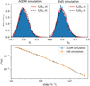Fig. 1. Statistical properties of the simulated cosmic overdensity field. Top: measured distribution of the δw overdensity field and the fln(δw, σ) lognormal distribution function for L = 60 Mpc h−1 cubic windows in our ΛCDM and EdS simulations at z = 0 redshift. We plotted the Gaussian approximation of the density field as a dashed black curve. Bottom: measured σ2 variance of the δw field as a function of the window volume at z = 0.

3. The power spectrum within finite volumes

The power spectrum of the δ(x) overdensity field is defined by

$$\begin{array}{c}\hfill {(2\pi )}^{3}P(\mathit{k}){\delta }_{\mathrm{D}}^3(\mathit{k}-{\mathit{k}}^{\prime })=\langle \delta (\mathit{k})\delta ({\mathit{k}}^{\prime })\rangle ,\end{array}$$(5)

where δ(k) is the Fourier transform of the δ(x) field and ${\delta }_{\text{D}}^3(\mathit{k})$ is the three-dimensional Dirac-delta function. This function contains all information from the statistics of the density field in the linear regime, and a decreasing fraction of the total information on smaller scales, if initial density fields followed Gaussian statistics. Since we assume that the Universe is isotropic, P(k) depends only on the length of the k vector and is thus denoted as P(k).

We adapted the definition by Chiang et al. (2014) for the position-dependent power spectrum. For the rest of the paper we use the cubic window function

$$\begin{array}{c}\hfill W_{\mathrm{L}}(\mathit{x})={\displaystyle \prod _{i=1}^3\theta (x_i),\text{where}\theta (x_i)=\{\begin{array}{cc}1\hfill & \text{if}|x_i|<L/2\hfill \\ 0\hfill & \text{otherwise}\hfill \end{array},}\end{array}$$(6)

where L is the linear size and x is a comoving coordinate vector. The local Fourier transform of the density field in this case is

$$\begin{array}{c}\hfill \delta (\mathit{k},{\mathit{r}}_w,L)={\displaystyle \int }{d}^{3}x\delta (\mathit{x})W_L(\mathit{x}-{\mathit{r}}_w){\mathrm{e}}^{-i\mathit{k}\mathit{x}},\end{array}$$(7)

where r_w is the comoving coordinate of the center of the survey. The position-dependent power spectrum inside the survey volume is then constructed as

$$\begin{array}{c}\hfill P_w(k,{\mathit{r}}_w,L)=\frac{1}{V}\langle |\delta (\mathit{k},{\mathit{r}}_w,L){|}^2\rangle ,\end{array}$$(8)

where V = L³ is the volume of the cubic survey. The local power spectrum definition above assumes that the mean cosmic mass density is known for the power spectrum analysis. This is true for simulations, but not for real surveys. If the global density is unknown, it is estimated from the average density inside the survey window, and the

$$\begin{array}{c}\hfill \stackrel{\sim }{\delta }(k)=\frac{\delta (k)}{1+{\delta }_w}\end{array}$$(9)

field is used in the power spectrum calculation instead of δ(k) (de Putter et al. 2012). This causes a bias in the power spectrum estimation, and the power spectrum in the survey window becomes

$$\begin{array}{c}\hfill P_{\mathit{sw}}(k)=\frac{1}{{(1+{\delta }_w)}^2}{P}_w(k),\end{array}$$(10)

where P_w(k) is the local power spectrum defined above. This effect on the measurements is called the local average effect. Since we work with simulations in this paper, we used the P_w(k) local power spectrum calculated by the known $\overline{\rho }$ average density unless otherwise stated.

The power spectrum and the position-dependent power spectrum evolves over time. There are two commonly used methods available to predict the power spectrum from an initial state at a later time: PT and numerical simulations of structure formation. The former are accurate early on or on the largest scales for late cosmological times, when structure formation is linear or mildly nonlinear. In the nonlinear regime, only the numerical simulations and the halo model yield precise predictions.

The evolution of the local power spectrum at coordinate r_w within volume V is determined by the cosmological parameters, the initial fluctuations, the overdensity inside the window (δ_w), and the tidal fields originating from outside the survey area. It is a difficult task to calculate these effects properly in the nonlinear regime. For simplicity, we neglected tidal fields and modeled the ratio of the position-dependent power spectrum and the global power spectrum as

$$\begin{array}{c}\hfill P_w(k,t|{\delta }_w,\sigma (V))=R(k,t,{\delta }_w,\sigma (V))P(k,t),\end{array}$$(11)

where σ²(V) is the variance of the overdensity field on the scale of the window function and R(k, t, δ_w, σ(V)) is the response function. It quantifies the response of the position-dependent power spectrum to the presence of a large-scale overdensity (δ_w) inside the window (Chiang et al. 2014; Wagner et al. 2015b).

By definition, the position-dependent power spectrum for every sub-volume, V, should average – after deconvolving the window function – to the global power spectrum. Thus, the response function fulfills

$$\begin{array}{c}\hfill 1=\frac{\langle P_w(k,t|{\delta }_w,V)\rangle }{P(k,t)}={\displaystyle \int }R(k,t,{\delta }_w,\sigma (V))f({\delta }_w,\sigma (V))\mathrm{d}{\delta }_w,\end{array}$$(12)

where f(δ_w, σ(V)) is the probability density-distribution function of the overdensity field on the scale of the window function.

In SPT, the effect of the overdensities are described as a function of the δ_L0D(t) linearly extrapolated Lagrangian overdensity,

$$\begin{array}{c}\hfill P(k,t|D(t){\delta }_{L0})={\displaystyle \sum _{n=0}^{\infty }\frac{1}{n!}{R}_{\mathcal{L},n}(k,t){\left[{\delta }_{L0}D(t)\right]}^n\overline{P}(k,t),}\end{array}$$(13)

where δ_L0 is the initial overdensity, D(t) is a linear growth function, and

$$\begin{array}{c}\hfill R_{\mathcal{L},n}(k,t)={\frac{1}{\overline{P}(k,t)}\frac{{\mathrm{d}}^{n}P(k,t|{\delta }_{L0}D(t))}{\mathrm{d}{\left({\delta }_{L0}D(t)\right)}^n}|}_{{\delta }_{L0}D(t)=0}\end{array}$$(14)

is the nth-order response function, with the zeroth order set to R_ℒ, 0(k, t) = 1 (Wagner et al. 2015b). An initially Gaussian field is assumed, and therefore the distribution of the linearly extrapolated density field is Gaussian too. Each power of the extrapolated overdensity is zero for a sub-volume with an average density. The consequence of this fact is that any order SPT response that uses this Taylor expansion will predict a power spectrum that is identical to the global one for average density sub-volumes.

The first two orders of the response function are the following:

$$\begin{array}{c}\hfill R_{\mathcal{L},1}=\frac{47}{21}-\frac{1}{3}\frac{\mathrm{d}lnP(k)}{\mathrm{d}lnk}\end{array}$$(15)

$$\begin{array}{c}\hfill R_{\mathcal{L},2}=\frac{8420}{1323}-\frac{100}{63}\frac{k}{P(k)}\frac{\mathrm{d}P(k)}{\mathrm{d}k}+\frac{1}{9}\frac{k^2}{P{(k)}^2}\frac{{\mathrm{d}}^{2}P(k)}{\mathrm{d}{k}^2}\end{array}$$(16)

The Eulerian responses can be calculated for the EdS Universe as

$$\begin{array}{cc}& R_1(k)=R_{\mathcal{L},1}(k)\hfill \end{array}$$(17)

$$\begin{array}{cc}& R_2(k)=R_{\mathcal{L},2}(k)-\frac{34}{21}{R}_{\mathcal{L},1}(k)\hfill \end{array}$$(18)

(Wagner et al. 2015b). As we show next, these results fit cosmological simulations well on scales where the probability distribution of the overdensity, δ, is nearly Gaussian.

The response function constructed from R₀ and R₁ fulfills Eq. (12) for a Gaussian distribution. While this is no longer true for higher-order SPT, the average should converge to one with increasing orders.

4. Response function from cosmological simulations

We expect the PT responses to accurately predict the position-dependent power spectra when δ_w is sufficiently close to zero and the density field is close to a Gaussian. If the survey window is too small, the skewness of the probability density function distorts the responses. In particular, the power spectrum of the average density sub-volumes might differ from the spectrum of the full cosmological volume due to non-Gaussianity.

To test this hypothesis, we calculated the position-dependent power spectra in a large number of sub-volumes from the simulations shown earlier. We divided the simulation volume into $N_{\text{cut}}^3$ distinct cubic sub-volumes with L = L_box/N_cut side lengths, similarly to Chiang et al. (2014). The position-dependent power spectra and the full-volume spectrum for L = 60 Mpc h⁻¹ in a ΛCDM simulation is shown in Fig. 2.

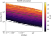Fig. 2. Position-dependent power spectra in our ΛCDM simulation at z = 0 with a L = 60 Mpc h−1 window size. The color represents the average density of each sub-volume. The full-volume power spectrum is plotted as a green curve for reference.

Compared to the global spectrum, the position-dependent spectra are only shifted by a constant factor for the k > 0.3 Mpc h⁻¹ region, suggesting that the overdensity response function is at most extremely weakly dependent on the k wavenumber. Motivated by this, we neglected any k dependence and defined the response for the i-th sub-volume as

$$\begin{array}{cc}\hfill R_{\text{sim,}i}({\delta }_w,L,t)& ={\langle \frac{P_{w,i}(k,{\delta }_w,L,t)}{P(k,t)}\rangle }_{k_{\min }<k<k_{\max }}\hfill \\ \hfill & =\frac{1}{k_{\max }-k_{\min }}{\displaystyle \underset{k_{\min }}{\overset{k_{\max }}{\int }}\mathrm{d}k\frac{P_{w,i}(k,{\delta }_w,L,t)}{P(k,t)},}\hfill \end{array}$$(19)

where ⟨⟩_k denotes k-average. Since the position-dependent power spectrum is sampled on discrete k_j values in our case, Eq. (19) becomes

$$\begin{array}{c}\hfill R_{\text{sim,}i}({\delta }_w,L,t)=\frac{1}{N_k}{\displaystyle \sum _{k_{\min }<k_j<k_{\max }}\frac{P_{w,i}(k_j,{\delta }_w,L,t)}{P(k_j,t)},}\end{array}$$(20)

where N_k is the number of k_j modes that satisfy k_min < k_j < k_max. The k_min and k_max values were set to max(16⋅π/L,0.3 Mpc⁻¹ h) and 1.5 Mpc⁻¹ h, respectively, to minimize the effect of the window function and the discreteness of the particles. The measured R_{sim, i}(δ_w, L, t) is shown along with the SPT responses in Fig. 3. The first- and second-order perturbative responses were calculated by assuming a power law for P(k), and by calculating k-average between k_min and k_max. The power-law approximations were valid in all measured k ranges. According to a visual inspection, the SPT response is consistent with the measured one in the larger windows when the overdensity, δ_w, is not far from zero. In smaller windows, especially for negative overdensities, SPT is far off, not even obeying the positivity constraint. Motivated by Fig. 3, we propose a new power-law fit for the response function,

$$\begin{array}{c}\hfill R({\delta }_w,\sigma )=B(\sigma ){({\delta }_w+1)}^{A(\sigma )}.\end{array}$$(21)

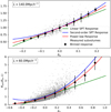Fig. 3. Simulated responses from our ΛCDM simulation with two different L window sizes at z = 0. The small gray markers represent the measured sub-volumes. This data have been re-binned, and the black circles with error bars represent the average response in each bin and the 1σ deviation. The linear (R = 1 + R1δw) and second-order ($R=1+R_1{\delta }_w+R_2{\delta }_w^2$) responses from SPT are plotted with the green and blue curves, respectively. The red curves represent the new, σ-dependent power-law response.

Since our goal is to predict the response from cosmological parameters, we express the dependence on the scale L as a function of σ dependence since σ(V)=σ(L³) is a known bijective function given a cosmological model. The response in this form is always positive when δ_w > −1, and it fits the simulated responses at all scales and overdensities. Our next objective was to calculate the B(σ) and A(σ) functions.

We required our fit to be compatible with the linear-order responses from SPT for low δ_w overdensity and large scales. Thus,

$$\begin{array}{c}\hfill {\frac{\mathrm{d}R({\delta }_w,\sigma )}{\mathrm{d}{\delta }_w}|}_{{\delta }_w=0}=R_1=\frac{47}{21}-\frac{1}{3}\frac{\mathrm{d}lnP(k)}{\mathrm{d}lnk}.\end{array}$$(22)

Therefore, B(σ) and A(σ) are not independent, and Eq. (21) takes the

$$\begin{array}{c}\hfill R({\delta }_w,\sigma )=B(\sigma ){({\delta }_w+1)}^{R_1/B(\sigma )}\end{array}$$(23)

form. For a late time ΛCDM cosmology beyond the weak linear regime, $\frac{\mathrm{d}lnP(k)}{\mathrm{d}lnk}$ is well approximated by −1 (Carron & Szapudi 2013).

The sub-volume power spectra should average to the global power spectrum. Using the lognormal probability density function for δ_w, the consistency requirement of Eq. (12) for our response function becomes

$$\begin{array}{c}\hfill B(\sigma )·{\mathrm{e}}^{\frac{{\sigma }^2}{2}[{\left(\frac{R_1}{B(\sigma )}\right)}^2-\frac{R_1}{B(\sigma )}]}=1.\end{array}$$(24)

This equation determines the B(σ) function. This is a transcendental equation with no known analytical solution. We used numerical solutions to calculate the responses in Figs. 3 and 5. Approximate solutions can be derived from Taylor series. The detailed calculations are in Appendix A. The first-order approximate solution suffices for most applications:

$$\begin{array}{c}\hfill B_I(\sigma )=1-\frac{1-{\mathrm{e}}^{-\frac{1}{2}{\sigma }^2(R_1^2-R_1)}}{(\frac{1}{2}{\sigma }^2(R_1-2R_1^2)+1)}·\end{array}$$(25)

The error of this approximation is below one percent for scales where σ < 0.24. This solution can be further approximated by expanding it as

$$\begin{array}{c}\hfill B(\sigma )\simeq 1-\frac{1}{2}{\sigma }^2{R}_1(R_1-1)\simeq 1-2{\sigma }^2(\text{for}\frac{\mathrm{d}lnP(k)}{\mathrm{d}lnk}\simeq -1).\end{array}$$(26)

This is accurate for window sizes with σ < 0.1 with sub-percent error. The median for the log-normal density field defined in Eq. (2) is

$$\begin{array}{c}\hfill \text{median}({\delta }_w)={\mathrm{e}}^{-\frac{1}{2}{\sigma }^2}-1.\end{array}$$(27)

Using the Taylor expansion of Eqs. (26) and (27), the connection between the super survey bias and the median of the overdensity field can be written as

$$\begin{array}{c}\hfill B\simeq 1+4·\text{median}({\delta }_w).\end{array}$$(28)

To test the effect of the k_min and k_max in Eq. (20), we binned the calculated responses into N_b = 13 equally spaced δ_w bins for multiple (k_min, k_max) pairs and calculated the

$$\begin{array}{c}\hfill {\chi }^2(k_{\min },k_{\max })={\displaystyle \sum _{i=0}^{N_{\mathrm{b}}}\frac{{(R_{\mathrm{theory}}({\delta }_i)-R_{\mathrm{sim},i}(k_{\min },k_{\max }))}^2}{{\sigma }_{\mathrm{sim},i}^2(k_{\min },k_{\max })}}\end{array}$$(29)

quantity for the second-order SPT and the new power-law responses, where R_sim, i is the average response inside the δ_i bin and ${\sigma }_{\text{sim},i}^2$ is the variance of the simulated response. The calculated χ²(k_min, k_max) showed that our power-law response fits the simulated responses significantly better compared to the second-order SPT response, and the goodness of this fit only mildly depends on the chosen (k_min, k_max) pairs. This can be seen in Fig. 4.

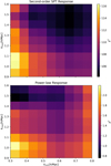Fig. 4. Comparison of the goodness of the fit of the theoretical responses in the L = 60 Mpc h−1 window size at z = 0. The new power-law response function fits the simulated responses significantly better.

Our proposed power-law fit and its approximations work in all regimes, even where the SPT approximation breaks down, despite having the same number of parameters as the second-order SPT. While SPT does a good job in both ΛCDM and in EdS cosmology for high density sub-volumes, it fails catastrophically for low density regions, for the first and second order. These are most of the sub-volumes due to the lognormal distribution of overdensities, and this is exactly where our proposed fit works significantly better than any previous approach. Higher-order SPT responses can achieve better fits (Wagner et al. 2015a), but they are significantly more complicated compared to this new formula.

Another physical consequence of the lognormal density field distribution and the power-law response is the bias of the power spectrum in the average density sub-volumes. According to Eqs. (11) and (21), the δ = 0 volumes on average have P_w(k, t|δ_w = 0, σ)=B(σ)P(k, t) as opposed to SPT, where these regions have the same spectrum as the full-volume one. To test this this prediction, we plotted the simulated responses of the δ_w = 0 bins from Fig. 5 as a function of the σ deviation with the B(σ) responses in Fig. 6. The simulated δ_w = 0 bias in the position-dependent power spectrum agrees well with the prediction of the power-law responses in ΛCDM and EdS cosmology.

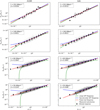Fig. 5. Simulated and theoretical responses in different window scales for two different cosmological models at z = 0. The new power-law response function fits the simulated responses well. Left: ΛCDM cosmology. Right: EdS cosmology.

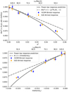Fig. 6. Simulated Rsim(δw = 0, σ) responses for ΛCDM and EdS cosmology. In contrast to SPT, the power-law response predicts that the mean density sub-volumes have smaller than average power spectra. This numeric B(σ2) prediction is plotted with a black curve and shows good agreement with the simulated responses in both cosmologies. Top: measured and predicted bias as a function of σ2. Bottom: bias as a function of the median sub-volume overdensity, ${\mathrm{e}}^{-\frac{1}{2}{\sigma }^2}-1$.

4.1. Redshift dependence

The SPT responses defined in Eq. (14) are dependent on the derivatives of the global power spectrum. As a consequence, these responses depend on the redshift since the power spectrum changes over time. Since we only used the first-order result in our new power-law response, Eq. (21) depends only on the redshift through $\frac{\mathrm{d}lnP(k)}{\mathrm{d}lnk}(z)$ and through σ_L(z) for a given L scale. We expect that the new power-law response can be universally used for all redshifts if the above redshift dependences are correctly taken into account. To test this hypothesis, we calculated the responses at z = 1 and 3 values for the L = 60 Mpc h⁻¹ window size from our ΛCDM simulation. As can be seen in Fig. 7, the calculated responses agree well with the power-law response function. The σ(z) variance of the density field distribution is a monotonically decreasing function of redshift for a given scale. The lognormal density distribution defined in Eq. (2) converges to Gaussian as the redshift increases and, as a consequence, the difference between perturbative and power-law response predictions decreases.

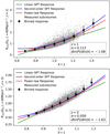Fig. 7. Simulated and theoretical Rsim(δw, σ, z) responses in ΛCDM cosmology for the L = 60 Mpc h−1 window size at z = 1 and 3 redshifts. The new power-law response function fits the simulated responses well, especially in the low density regions. At higher redshifts, the SPT and power-law responses converge as the density field becomes more Gaussian.

4.2. Response inside surveys

As we stated earlier, there are two ways to calculate the local power spectrum: by using the global average $\overline{\rho }$ mass density, or by using the estimated ${\overline{\rho }}_{\mathit{sw}}=\overline{\rho }·(1+{\delta }_{\mathit{w}})$ mass density during the power spectrum calculation. The conversion between the two definitions can be done easily by using Eq. (10). In the majority of this paper, we used the former method because the global density was available in our simulations. However, for real surveys only the latter definition can be used. We used Eqs. (10) and (19) to calculate the

$$\begin{array}{cc}\hfill R_{\mathrm{sim},sw,i}({\delta }_w,L,t)& ={\langle \frac{P_{sw,i}(k,{\delta }_w,L,t)}{P(k,t)}\rangle }_{k_{\min }<k<k_{\max }}\hfill \\ \hfill & =\frac{1}{{(1-{\delta }_w)}^2}{R}_{\mathrm{sim},i}({\delta }_w,L,t)\hfill \end{array}$$(30)

simulated survey responses in this case and plotted the results in Fig. 8 for ΛCDM and EdS cosmology.

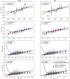Fig. 8. Simulated and theoretical responses in simulated surveys where the average mass density is unknown. The local average effect results in a (1 + δw)−2 bias in the power spectrum and in the response function compared to Fig. 5. The power-law response in this case is in good agreement with the simulated data. Left: ΛCDM cosmology. Right: EdS cosmology.

The theoretical responses also have to be scaled by 1/(1 + δ_w)² if the power spectrum is calculated from the estimated average mass density, and the power-law response in Eq. (23) thus becomes

$$\begin{array}{c}\hfill R_{\mathit{sw}}({\delta }_w,\sigma )=B(\sigma ){({\delta }_w+1)}^{[R_1/B(\sigma )-2]}.\end{array}$$(31)

We plot the scaled theoretical responses in Fig. 8. We note that the bias described by the B(σ) function for δ_w = 0 average density surveys is also present in this case.

5. Conclusion

We have investigated the power spectrum response to overdensities in cosmological N-body simulations, paying special attention to the non-Gaussian effects of the density field distribution. Standard perturbation theory predicts the measured responses on scales where the PDF of the density field is close to a Gaussian distribution. For smaller window sizes, where the distribution is more lognormal, the simulated responses did not match the first- and second-order SPT predictions, especially for small overdensities. Motivated by this:

1. We have calculated the effect of the density distribution on a general overdensity response function.

2. We have shown that this causes a bias for δ_w = 0, even in small volumes, due to the lognormal distribution of densities.

3. We have introduced a phenomenological power-law response function for the position-dependent power spectrum by combining the first-order SPT result with the constrains of the lognormal density distribution, and we have demonstrated its accuracy on cosmological N-body simulations.

The new response function is straightforward to calculate using standard tools from cosmological parameters, and it provides an extremely accurate prediction for the local power spectrum. In particular, it is especially useful for low density regions, which includes most of the Universe due to log-normality, where low-order SPT fails catastrophically.

A useful application of our formula would be to correct the measured small-scale power spectrum in zoom-in simulations, with or without the combination of the phase inversion method described by Angulo & Pontzen (2016), to reduce the effects of the cosmic variance. Our formulas correct the local power spectrum even for an average density simulation, where the SPT approach predicts no bias.

Our fit predicts a super survey bias of B(σ)≃1 − 2σ² at z = 0, the accuracy of which was verified in the simulations. This is a consequence of the skewed (lognormal) distribution of the overdensities: a typical sub-volume will be underdense, and the average density sub-volume will have a power spectrum bias of order −2σ². In the Gaussian approximation, the k_max of the sub-volume would determine the errors on the overall power spectrum amplitude, and thus this bias would always be significant. In reality, there is a plateau in the power spectrum information due to non-Gaussianity (Rimes & Hamilton 2006; Neyrinck et al. 2006) that limits the accuracy that is achievable with two-point statistics. Carron et al. (2014) identified the plateau σ_min, the minimum achievable super survey variance, as a quadrature sum of the super survey variance, ${\sigma }_{\mathrm{SS}}\simeq \frac{26}{21}\sigma (V)$ (local), and the intra-survey variance, σ_IS ≃ P(k_max)/V. The former alone is typically larger than the super survey bias identified here, which depends on the square of the variance. Therefore, in most practical cases with large enough sub-volumes of L ≳ 200 Mpc h⁻¹, the bias will be at the sub-percent level and smaller than the super survey variance.

The main consequence of the lognormal distribution and the power-law response is that the mean density volumes have power spectra that are smaller than the average, full-volume power spectrum.

Acknowledgments

This work was supported by the Ministry of Innovation and Technology NRDI Office grants OTKA NN 129148 and the MILAB Artificial Intelligence National Laboratory Program. IS acknowledges support from the National Science Foundation (NSF) award 1616974. GR’s research was supported by an appointment to the NASA Postdoctoral Program administered by Oak Ridge Associated Universities under contract with NASA. GR was supported by JPL, which is run under contract by California Institute of Technology for NASA. We thank A. S. Szalay for insightful suggestions and comments.

References

Appendix A: Approximate B(σ) functions

For a general overdensity response function, R(k, δ_w, σ), the average power spectrum in lognormal density distribution can be calculated as

$$\begin{array}{c}\hfill \langle P_w(k,\sigma )\rangle ={\displaystyle \underset{-1}{\overset{\infty }{\int }}R(k,{\delta }_w,\sigma )P(k)f_{\mathit{ln}}({\delta }_w,\sigma )d{\delta }_w.}\end{array}$$(A.1)

Since the average sub-volume spectrum is equal to the full-volume spectrum, Eq. A.1 can be simplified as

$$\begin{array}{c}\hfill 1={\displaystyle \underset{-1}{\overset{\infty }{\int }}R(k,{\delta }_w,\sigma )f_{\mathit{ln}}({\delta }_w,\sigma )d{\delta }_w.}\end{array}$$(A.2)

With our power-law assumption,

$$\begin{array}{c}\hfill R({\delta }_w,\sigma )=B(\sigma ){({\delta }_w+1)}^{R_1/B(\sigma )},\end{array}$$(A.3)

for the response function, the integral on the right side of Eq. A.1 can be solved analytically. The equation then becomes

$$\begin{array}{c}\hfill 1=B(\sigma )·e^{\frac{{\sigma }^2}{2}[{\left(\frac{R_1}{B(\sigma )}\right)}^2-\frac{R_1}{B(\sigma )}]}.\end{array}$$(A.4)

This transcendental equation has no known analytical solution for B(σ), but approximate solutions can be constructed using Taylor series. If we define the

$$\begin{array}{c}\hfill G(B):=B(\sigma )·e^{\frac{{\sigma }^2}{2}[{\left(\frac{R_1}{B(\sigma )}\right)}^2-\frac{R_1}{B(\sigma )}]}-1\end{array}$$(A.5)

function, Eq A.4 can be written as

$$\begin{array}{c}\hfill 0={\displaystyle \sum _{n=0}^{\infty }{\frac{1}{n!}\frac{d^{n}G(B)}{d{B}^n}|}_{B=1}·{(B-1)}^n.}\end{array}$$(A.6)

An approximate solution that uses the first few terms of this Taylor expansion around B = 1 is expected to be close to the real solution for small σ values since B(σ) = 1 when σ = 0. The first two derivatives of G(A) are

$$\begin{array}{c}\hfill \frac{d}{\mathit{dB}}G(B)=(\frac{1}{2}{\sigma }^2(\frac{R_1}{B}-\frac{2{R_1}^2}{B^2})+1)e^{\frac{1}{2}{\sigma }^2(\frac{{R_1}^2}{B^2}-\frac{R_1}{B})}\end{array}$$(A.7)

$$\begin{array}{c}\hfill \frac{d^2}{d{B}^2}G(B)=(\frac{1}{4}{\sigma }^{4}B{(\frac{R_1}{B^2}-\frac{2{R_1}^2}{B^3})}^2+{\sigma }^2\frac{{R_1}^2}{B^3})e^{\frac{1}{2}{\sigma }^2(\frac{{R_1}^2}{B^2}-\frac{R_1}{B})}.\end{array}$$(A.8)

Using these, different orders of polynomial equations can be constructed for B(σ). For n ≤ 1, the first-order equation can be written as

$$\begin{array}{cc}& e^{\frac{1}{2}{\sigma }^2(R_1^2-R_1)}-1+\hfill \\ \hfill & +\left[(\frac{1}{2}{\sigma }^2(R_1-2R_1^2)+1)e^{\frac{1}{2}{\sigma }^2(R_1^2-R)}\right](B_I(\sigma )-1)=0,\hfill \end{array}$$(A.9)

where the first-order solution is

$$\begin{array}{c}\hfill B_I(\sigma )=1-\frac{1-e^{-\frac{1}{2}{\sigma }^2(R_1^2-R_1)}}{(\frac{1}{2}{\sigma }^2(R_1-2R_1^2)+1)}.\end{array}$$(A.10)

The n ≤ 2 equation is

$$\begin{array}{cc}& e^{\frac{1}{2}{\sigma }^2(R_1^2-R_1)}-1+\hfill \\ \hfill & +\left[(\frac{1}{2}{\sigma }^2(R_1-2R_1^2)+1)e^{\frac{1}{2}{\sigma }^2(R_1^2-R_1)}\right](B_{\mathit{II}}(\sigma )-1)+\hfill \\ \hfill & +\frac{1}{2}\left[(\frac{1}{4}{\sigma }^4{(R_1-2R_1^2)}^2+{\sigma }^2{R}_1^2)e^{\frac{1}{2}{\sigma }^2(R_1^2-R_1)}\right]{(B_{\mathit{II}}(\sigma )-1)}^2=0,\hfill \end{array}$$(A.11)

and the solution is

$$\begin{array}{cc}& B_{\mathit{II}}(\sigma )=1-\frac{1}{\left[(\frac{1}{4}{\sigma }^4{(R_1-2R_1^2)}^2+{\sigma }^2{R}_1^2)e^{\frac{1}{2}{\sigma }^2(R_1^2-R_1)}\right]}·\hfill \\ \hfill & ·(\left[(\frac{1}{2}{\sigma }^2(R_1-2R_1^2)+1)e^{\frac{1}{2}{\sigma }^2(R_1^2-R_1)}\right]+\hfill \\ \hfill & +({\left[(\frac{1}{2}{\sigma }^2(R_1-2R_1^2)+1)e^{\frac{1}{2}{\sigma }^2(R_1^2-R_1)}\right]}^2-\hfill \\ \hfill & {-2\left[(\frac{1}{4}{\sigma }^4{(R_1-2R_1^2)}^2+{\sigma }^2{R}_1^2)e^{\frac{1}{2}{\sigma }^2(R_1^2-R_1)}\right](e^{\frac{1}{2}{\sigma }^2(R_1^2-R_1)}-1))}^{\frac{1}{2}}).\hfill \end{array}$$(A.12)

The first- and second-order solutions can be seen in the top panel of Fig. A.1. The precision of these solutions can be checked by substituting B(σ) back into Eq. A.4. This is plotted in the bottom panel of Fig. A.1.

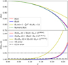Fig. A.1. Approximate super survey biases. Top: Approximate BI(σ) and BII(σ) solutions with the numeric B(σ) function. Bottom: Error in the average of the RI(δw, σ) and RII(δw, σ) responses generated from the BI(σ) and BII(σ) functions, respectively. We have adopted R1 = 47/21 + 1/3 for this plot.

All Tables

All Figures

Fig. 1. Statistical properties of the simulated cosmic overdensity field. Top: measured distribution of the δw overdensity field and the fln(δw, σ) lognormal distribution function for L = 60 Mpc h−1 cubic windows in our ΛCDM and EdS simulations at z = 0 redshift. We plotted the Gaussian approximation of the density field as a dashed black curve. Bottom: measured σ2 variance of the δw field as a function of the window volume at z = 0.

In the text

	Fig. 2. Position-dependent power spectra in our ΛCDM simulation at z = 0 with a L = 60 Mpc h−1 window size. The color represents the average density of each sub-volume. The full-volume power spectrum is plotted as a green curve for reference.
In the text

Fig. 3. Simulated responses from our ΛCDM simulation with two different L window sizes at z = 0. The small gray markers represent the measured sub-volumes. This data have been re-binned, and the black circles with error bars represent the average response in each bin and the 1σ deviation. The linear (R = 1 + R1δw) and second-order ($R=1+R_1{\delta }_w+R_2{\delta }_w^2$) responses from SPT are plotted with the green and blue curves, respectively. The red curves represent the new, σ-dependent power-law response.

In the text

	Fig. 4. Comparison of the goodness of the fit of the theoretical responses in the L = 60 Mpc h−1 window size at z = 0. The new power-law response function fits the simulated responses significantly better.
In the text

	Fig. 5. Simulated and theoretical responses in different window scales for two different cosmological models at z = 0. The new power-law response function fits the simulated responses well. Left: ΛCDM cosmology. Right: EdS cosmology.
In the text

Fig. 6. Simulated Rsim(δw = 0, σ) responses for ΛCDM and EdS cosmology. In contrast to SPT, the power-law response predicts that the mean density sub-volumes have smaller than average power spectra. This numeric B(σ2) prediction is plotted with a black curve and shows good agreement with the simulated responses in both cosmologies. Top: measured and predicted bias as a function of σ2. Bottom: bias as a function of the median sub-volume overdensity, ${\mathrm{e}}^{-\frac{1}{2}{\sigma }^2}-1$.

In the text

	Fig. 7. Simulated and theoretical Rsim(δw, σ, z) responses in ΛCDM cosmology for the L = 60 Mpc h−1 window size at z = 1 and 3 redshifts. The new power-law response function fits the simulated responses well, especially in the low density regions. At higher redshifts, the SPT and power-law responses converge as the density field becomes more Gaussian.
In the text

	Fig. 8. Simulated and theoretical responses in simulated surveys where the average mass density is unknown. The local average effect results in a (1 + δw)−2 bias in the power spectrum and in the response function compared to Fig. 5. The power-law response in this case is in good agreement with the simulated data. Left: ΛCDM cosmology. Right: EdS cosmology.
In the text

	Fig. A.1. Approximate super survey biases. Top: Approximate BI(σ) and BII(σ) solutions with the numeric B(σ) function. Bottom: Error in the average of the RI(δw, σ) and RII(δw, σ) responses generated from the BI(σ) and BII(σ) functions, respectively. We have adopted R1 = 47/21 + 1/3 for this plot.
In the text

References

- Aihara, H., Arimoto, N., Armstrong, R., et al. 2018, PASJ, 70, S4 [NASA ADS] [Google Scholar]
- Akitsu, K., & Takada, M. 2018, Phys. Rev. D, 97, 063527 [NASA ADS] [CrossRef] [Google Scholar]
- Akitsu, K., Li, Y., & Okumura, T. 2021, J. Cosmol. Astropart. Phys., 2021, 041 [CrossRef] [Google Scholar]
- Allgood, B., Blumenthal, G., & Primack, J. R. 2001, ArXiv e-prints [arXiv:astro-ph/0109403] [Google Scholar]
- Angulo, R. E., & Pontzen, A. 2016, MNRAS, 462, L1 [NASA ADS] [CrossRef] [Google Scholar]
- Barreira, A., Krause, E., & Schmidt, F. 2018a, J. Cosmol. Astropart. Phys., 2018, 053 [CrossRef] [Google Scholar]
- Barreira, A., Krause, E., & Schmidt, F. 2018b, J. Cosmol. Astropart. Phys., 2018, 015 [Google Scholar]
- Barreira, A., Nelson, D., Pillepich, A., et al. 2019, MNRAS, 488, 2079 [NASA ADS] [CrossRef] [Google Scholar]
- Baugh, C. M., & Efstathiou, G. 1994, MNRAS, 267, 323 [NASA ADS] [Google Scholar]
- Beck, R., McPartland, C., Repp, A., Sanders, D., & Szapudi, I. 2020, MNRAS, 493, 2318 [NASA ADS] [CrossRef] [Google Scholar]
- Carron, J., & Szapudi, I. 2013, MNRAS, 434, 2961 [NASA ADS] [CrossRef] [Google Scholar]
- Carron, J., Wolk, M., & Szapudi, I. 2014, MNRAS, 444, 994 [NASA ADS] [CrossRef] [Google Scholar]
- Castorina, E., & Moradinezhad Dizgah, A. 2020, J. Cosmol. Astropart. Phys., 2020, 007 [CrossRef] [Google Scholar]
- Chambers, K. C., Magnier, E. A., Metcalfe, N., et al. 2016, ArXiv e-prints [arXiv:1612.05560] [Google Scholar]
- Chan, K. C., Moradinezhad Dizgah, A., & Noreña, J. 2018, Phys. Rev. D, 97, 043532 [NASA ADS] [CrossRef] [Google Scholar]
- Chiang, C.-T., Wagner, C., Schmidt, F., & Komatsu, E. 2014, J. Cosmol. Astropart. Phys., 2014, 048 [CrossRef] [Google Scholar]
- Coles, P., & Jones, B. 1991, MNRAS, 248, 1 [NASA ADS] [CrossRef] [Google Scholar]
- Crocce, M., Pueblas, S., & Scoccimarro, R. 2006, MNRAS, 373, 369 [NASA ADS] [CrossRef] [Google Scholar]
- Crocce, M., Pueblas, S., & Scoccimarro, R. 2012, Astrophysics Source Code Library [record ascl:1201.005] [Google Scholar]
- Dawson, K. S., Schlegel, D. J., Ahn, C. P., et al. 2013, AJ, 145, 10 [Google Scholar]
- de Putter, R., Wagner, C., Mena, O., Verde, L., & Percival, W. J. 2012, J. Cosmol. Astropart. Phys., 2012, 019 [CrossRef] [Google Scholar]
- DESI Collaboration (Aghamousa, A., et al.) 2016, ArXiv e-prints [arXiv:1611.00036] [Google Scholar]
- Digman, M. C., McEwen, J. E., & Hirata, C. M. 2019, J. Cosmol. Astropart. Phys., 2019, 004 [CrossRef] [Google Scholar]
- Doré, O., Bock, J., Ashby, M., et al. 2014, ArXiv e-prints [arXiv:1412.4872] [Google Scholar]
- Green, J., Schechter, P., Baltay, C., et al. 2012, ArXiv e-prints [arXiv:1208.4012] [Google Scholar]
- Katz, N., & White, S. D. M. 1993, ApJ, 412, 455 [NASA ADS] [CrossRef] [Google Scholar]
- Lacasa, F., & Grain, J. 2019, A&A, 624, A61 [NASA ADS] [CrossRef] [EDP Sciences] [Google Scholar]
- Li, Y., Hu, W., & Takada, M. 2014, Phys. Rev. D, 89, 083519 [NASA ADS] [CrossRef] [Google Scholar]
- LSST Science Collaboration (Abell, P. A., et al.) 2009, ArXiv e-prints [arXiv:0912.0201] [Google Scholar]
- Masaki, S., Nishimichi, T., & Takada, M. 2020, MNRAS, 496, 483 [NASA ADS] [CrossRef] [Google Scholar]
- Neyrinck, M. C., Szapudi, I., & Rimes, C. D. 2006, MNRAS, 370, L66 [NASA ADS] [CrossRef] [Google Scholar]
- Oñorbe, J., Garrison-Kimmel, S., Maller, A. H., et al. 2014, MNRAS, 437, 1894 [CrossRef] [Google Scholar]
- Percival, W. J., Baugh, C. M., Bland-Hawthorn, J., et al. 2001, MNRAS, 327, 1297 [Google Scholar]
- Planck Collaboration XIII. 2016, A&A, 594, A13 [NASA ADS] [CrossRef] [EDP Sciences] [Google Scholar]
- Rácz, G., Szapudi, I., Csabai, I., & Dobos, L. 2018, MNRAS, 477, 1949 [CrossRef] [Google Scholar]
- Repp, A., & Szapudi, I. 2018, MNRAS, 473, 3598 [NASA ADS] [CrossRef] [Google Scholar]
- Rimes, C. D., & Hamilton, A. J. S. 2006, MNRAS, 371, 1205 [NASA ADS] [CrossRef] [Google Scholar]
- Rizzato, M., Benabed, K., Bernardeau, F., & Lacasa, F. 2019, MNRAS, 490, 4688 [NASA ADS] [CrossRef] [Google Scholar]
- Sato, T., Hütsi, G., Nakamura, G., & Yamamoto, K. 2013, Int. J. Astron. Astrophys., 3, 243 [CrossRef] [Google Scholar]
- Scoville, N., Aussel, H., Brusa, M., et al. 2007, ApJS, 172, 1 [Google Scholar]
- Springel, V. 2005, MNRAS, 364, 1105 [Google Scholar]
- Stücker, J., Schmidt, A. S., White, S. D. M., Schmidt, F., & Hahn, O. 2021, MNRAS, 503, 1473 [CrossRef] [Google Scholar]
- Takada, M., & Hu, W. 2013, Phys. Rev. D, 87, 123504 [NASA ADS] [CrossRef] [Google Scholar]
- Takahashi, R., Nishimichi, T., Takada, M., Shirasaki, M., & Shiroyama, K. 2019, MNRAS, 482, 4253 [NASA ADS] [CrossRef] [Google Scholar]
- Tamura, N., Takato, N., Shimono, A., et al. 2016, in Ground-based and Airborne Instrumentation for Astronomy VI, eds. C. J. Evans, L. Simard, & H. Takami, SPIE Conf. Ser., 9908, 99081M [NASA ADS] [Google Scholar]
- Tegmark, M., Blanton, M. R., Strauss, M. A., et al. 2004, ApJ, 606, 702 [Google Scholar]
- The Dark Energy Survey Collaboration 2005, ArXiv e-prints [arXiv:astro-ph/0510346] [Google Scholar]
- Tutusaus, I., Martinelli, M., Cardone, V. F., et al. 2020, A&A, 643, A70 [EDP Sciences] [Google Scholar]
- Vogeley, M. S. 1995, in Clustering in the Universe, eds. S. Maurogordato, C. Balkowski, C. Tao, & J. Tran Thanh Van, 13 [Google Scholar]
- Wagner, C., Schmidt, F., Chiang, C. T., & Komatsu, E. 2015a, MNRAS, 448, L11 [CrossRef] [Google Scholar]
- Wagner, C., Schmidt, F., Chiang, C.-T., & Komatsu, E. 2015b, J. Cosmol. Astropart. Phys., 2015, 042 [CrossRef] [Google Scholar]