| Issue |
A&A
Volume 661, May 2022
|
|
|---|---|---|
| Article Number | A118 | |
| Number of page(s) | 13 | |
| Section | Catalogs and data | |
| DOI | https://doi.org/10.1051/0004-6361/202142568 | |
| Published online | 24 May 2022 | |
Hunting for open clusters in Gaia EDR3: 628 new open clusters found with OCfinder★
1
Leiden Observatory, Leiden University,
Niels Bohrweg 2,
2333
CA Leiden,
The Netherlands
e-mail: This email address is being protected from spambots. You need JavaScript enabled to view it.
2
Dept. Física Quàntica i Astrofísica, Institut de Ciències del Cosmos (ICCUB), Universitat de Barcelona (IEEC-UB),
Martí i Franquès 1,
08028
Barcelona,
Spain
3
Max-Planck-Institut für Astronomie,
Königstuhl 17,
69117
Heidelberg,
Germany
4
Laboratoire d’Astrophysique de Bordeaux, Univ. Bordeaux, CNRS,
B18N, allée Geoffroy Saint-Hilaire,
33615
Pessac,
France
5
Barcelona Supercomputing Center (BSC),
Barcelona,
Spain
Received:
2
November
2021
Accepted:
15
February
2022
Abstract
Context. The improvements in the precision of the published data in Gaia EDR3 with respect to Gaia DR2, particularly for parallaxes and proper motions, offer the opportunity to increase the number of known open clusters in the Milky Way by detecting farther and fainter objects that have thus far gone unnoticed.
Aims. Our aim is to continue to complete the open cluster census in the Milky Way with the detection of new stellar groups in the Galactic disc. We use Gaia EDR3 up to magnitude G = 18 mag, increasing the magnitude limit and therefore the search volume explored in one unit with respect to our previous studies.
Methods. We used the OCfinder method to search for new open clusters in Gaia EDR3 using a big data environment. As a first step, OCfinder identified stellar statistical overdensities in five-dimensional astrometric space (position, parallax, and proper motions) using the DBSCAN clustering algorithm. Then, these overdensities were classified into random statistical overdensities or real physical open clusters using a deep artificial neural network trained on well-characterised G, GBP – GRP colour-magnitude diagrams.
Results. We report the discovery of 628 new open clusters within the Galactic disc, with most of them being located beyond 1 kpc from the Sun. From the estimation of ages, distances, and line-of-sight extinctions of these open clusters, we see that young clusters align following the Galactic spiral arms while older ones are dispersed in the Galactic disc. Furthermore, we find that most open clusters are located at low Galactic altitudes with the exception of a few groups older than 1 Gyr.
Conclusions. We show the success of the OCfinder method leading to the discovery of a total of 1274 open clusters (joining the discoveries here with the previous ones based on Gaia DR2), which represents almost 50% of the known population. Our ability to perform big data searches on a large volume of the Galactic disc, together with the higher precision in Gaia EDR3, enable us to keep completing the census with the discovery of new open clusters.
Key words: Galaxy: disk / open clusters and associations: general / astrometry / methods: data analysis
Full Table 1 and Table 2 are only available at the CDS via anonymous ftp to cdsarc.u-strasbg.fr (130.79.128.5) or via http://cdsarc.u-strasbg.fr/viz-bin/cat/J/A+A/661/A118
© ESO 2022
1 Introduction
Open clusters (OCs) have historically been used to study the structural, kinematical, and chemical properties of the disc of the Milky Way, and its evolution. For this reason, in recent years, there has been a growing interest in building an accurate and complete view of the OC population. In particular, after the Gaia Second Data Release (Gaia DR2, Gaia Collaboration 2018), the study of this field was revolutionised by the re-definition of the OC population, with Cantat-Gaudin et al. (2018) refusing around 50% of the OCs reported in pre-Gaia catalogues as not real OCs (Dias et al. 2002; Kharchenko et al. 2013). Furthermore, Gaia DR2 enabled the systematic detection of new OCs using machine-learning methods, which outperform traditional manual methods to search for these objects. Castro-Ginard et al. (2018, hereafter Paper I) were able to find 23 new OCs in Gaia DR1’s TGAS subset (Gaia Collaboration 2016; Michalik et al. 2015), and then they used the same methodology to detect more than 600 new OCs in the Galactic disc using Gaia DR2, which represents about one-third of the currently known OC population (Castro-Ginard et al. 2019, 2020, hereafter Paper II and Paper III, respectively). Since then, several publications have made use of machine-learning-based methods to detect new OCs (Cantat-Gaudin et al. 2019; Sim et al. 2019; Liu & Pang 2019; Ferreira et al. 2020; Hunt & Reffert 2021), computing membership lists (Cantat-Gaudin & Anders 2020; Jaehnig et al. 2021) or characterising their astrophysical properties (Bossini et al. 2019; Cantat-Gaudin et al. 2020; Dias et al. 2021).
Several studies have combined Gaia astrometry with ground-based radial velocities with the purpose of studying the kinematics of the OC population (e.g. Soubiran et al. 2018; Carrera et al. 2022). Tarricq et al. (2021) studied the 3D kinematics and age dependence of the OC population, also providing orbital parameters for 1382 OCs. Other studies have used OCs’ available astrometric and kinematic information to trace the spiral structure in the Milky Way (Dias & Lépine 2005). On this topic, Monteiro et al. (2021) found that the behaviour of the spiral arms could be explained by classical density waves. However, Castro Ginard et al. (2021) recently found a transient nature of the arms disfavouring classic density waves as the main drivers of the spiral structure, which is also supported by studies using tracers other than OCs (Minniti et al. 2021; Colombo et al. 2022). These contradicting results show the need to keep improving the OC census.
The coupling of Gaia data with the detailed abundance results of large spectroscopic surveys has allowed for a more complete picture of the chemical composition of the OC population to be sketched. In all of these studies, an unbiased and complete census of the OCs of the Milky Way is needed to tackle the chemical evolution of our Galaxy. Detailed chemical abundance radial gradients in the Milky Way and their age dependence have been characterised (e.g. Carrera et al. 2019; Spina et al. 2021). Temporal dependencies of chemical abundance ratios are commonly calibrated using OCs due to their precise age determination (Casamiquela et al. 2021b). Finally, OCs are used as test cases to explore the feasibility of a diversity of techniques such as strong chemical tagging, that is to say the possibility of finding stars that were born in the same star-forming event (Casamiquela et al. 2021a).
The latest release of Gaia data (EDR3, Gaia Collaboration 2021), providing astrometric measurements for about 1.8 billion stars with improved precision with respect to Gaia DR2, offers the opportunity to re-visit the OC census and keep improving it, both in terms of a better characterisation and new discoveries. The improved precisions in parallax, and particularly in proper motions with respect to Gaia DR2, allow for the application of machine-learning methods to search for new structures that would go unnoticed with traditional methods, which mostly relied on visual inspection. In this context, we adapted our methodology (developed and applied in Paper I, Paper II, and Paper III), which we dub OCfinder, to search for unknown OCs in Gaia EDR3 using its astrometric and photometric data.
This paper is organised as follows. In Sect. 2, we describe the data used to search for OCs. The OCfinder method used for that purpose is described in Sect. 3. Section 4 describes the OCs found, both re-detected and new findings. Finally, our conclusions are presented in Sect. 5.
2 Data
The data used in this paper to search for unknown OCs is Gaia EDR3 (Gaia Collaboration 2021). Gaia EDR3 is the first delivery of the third data release, and among other products it provides about 1.8 billion sources with astrometric and photometric observations, that is (l, b,  ,
,  ,µδ, G, GBP, GRP), with an improved precision with respect to Gaia DR2 due to an increase in the observational time baseline, now spanning a period of 34 months. Thanks to this improvement, we are able to search for new OCs with a deeper magnitude cut, which allows us to reach farther and less populated groupings. The adopted magnitude limit is G = 18 mag, unlike our previous studies where the limit was G = 17. Additionally, and since OCs are usually found in the Galactic disc, we limited our search to Galactic latitudes within |b| ≤ 20°, where most of the OCs are expected to be found. Similarly to our previous searches, we rejected stars with parallaxes larger than 7 mas to avoid very close OCs, which will suffer from strong projection effects and will not be detectable by our method, and sources with negative parallaxes. We also filtered out stars with proper motions higher than
  and |µδ| ≥ 30 mas yr−1 to remove stars incompatible with disc rotation, which OCs are expected to follow.
The median parallax uncertainty in Gaia EDR3 at G = 18 mag is 0.12 mas, while for proper motions the median uncertainties in  and µδ at G = 18 mag are of 0.123 and 0.111 mas yr−1, respectively (Lindegren et al. 2021). These are similar uncertainty levels in comparison to that of Gaia DR2 at magnitude G = 17 mag (Lindegren et al. 2018). For the photometry, the uncertainties in Gaia EDR3 at G = 18 mag are at the level of a thousandth for G, and a hundredth of a magnitude for GBP and GRP (Riello et al. 2021). These magnitude uncertainty levels are also comparable to Gaia DR2 at G = 17 mag; therefore we consider them to be a reasonable compromise to succesfully achieve our goals. Altogether, and taking the aforementioned filters into account, the sample to be analysed contains 232 463 114 sources, and its analysis is enabled thanks to the use of a big data environment in our data analysis pipeline (Castro-Ginard et al. 2020).
3 The OCfinder method
The methodology developed to search for new OCs in Gaia data, OCfinder, is described in detail in Paper I. It was successfully applied to detect 23 new nearby OCs (Castro-Ginard et al. 2018) in the TGAS data set of Gaia DR1. It was also applied to Gaia DR2 where 53 new OCs were detected in a direction near the Galactic anticentre (Castro-Ginard et al. 2019) and hundreds of new OCs in a big data search on the whole Galactic disc (CastroGinard et al. 2020).
The OCfinder method consists of two main steps. The first step is a blind search for overdensities in the five-dimensional astrometric space of Gaia, that is (l, b,  ,
,  , µδ), so as to find sets of stars which are more clustered than the average field stars for that region (Sect. 3.2). The second step makes use of the Gaia photometry to confirm whether OC member stars follow an isochrone pattern in a colour-magnitude diagram (CMD) using an artificial neural network trained on well-characterised CMDs (Sect. 3.3).
3.1 Data preparation
We divided the sky into small areas of size L × L deg2, where L varies according to the local structure density. This was done in order to define local average densities, accounting for the varying densities of the Galactic disc, when searching for representative overdensities which may correspond to physical OCs. In our methodology, the sizes of these regions are not defined by following computational, but physical arguments. We used the Gaia Universe Model Snapshot1 (GUMS, Robin et al. 2012) to represent the field star population, together with realistic OCs simulated using the Gaia Object Generator (GOG, Luri et al. 2014) both including errors at the time of Gaia EDR32, to find the size L of the regions that detect most of the simulated OCs (see Sect. 3 in Paper I for details). In this case, the sizes of the regions ranges from L = 10° to L = 15°, which corresponds to a maximum of about 107 stars per box to be simultaneously analysed with the clustering algorithm. The simultaneous analysis of such a large number of stars is not a problem for our method due to the inclusion of a big data environment (see details in Sect. 3.2).
Once the stars are divided into the L × L deg2 regions, the five astrometric dimensions (l, b,  ,
,  , µδ) are standardised in order to balance their importance in the clustering algorithm. In our case, we used the StandardScaler method implemented in the scikit-learn Python library (Pedregosa et al. 2011), which transforms each dimension to have zero mean and unit variance.
3.2 Astrometric clustering with DBSCAN
In each of the L × L deg2 regions, we ran the density-based clustering algorithm DBSCAN (Ester et al. 1996) to find statistical overdensities that may belong to real OCs. DBSCAN relies on two input parameters, which are e and minPts, to define a density threshold and it searches for overdensities above the threshold. As a brief description, DBSCAN visits each source in the dataset, builds an N-dimensional ϵ neighbourhood around the source, and counts how many sources are within the ϵ neighbourhood. If at least minPts sources are found, they are considered to be a cluster (we refer readers to Sect. 2 in Paper I for a DBSCAN description relevant for this application).
Similarly to our previous applications of OCfinder, we selected several optimal values of minPts which were found, together with L, using simulated data. In this case, the values of minPts range from eight to 16 stars. The computation of the e parameter was done automatically in each L × L deg2 region taking advantage of the fact that OC member stars are closer than random field stars in multidimensional space including positions, parallax, and proper motions. In brief, we computed the distribution of distances for each star to its kth nearest neighbour (defined as k = minPts − 1), and we compared it to the distribution of kth nearest neighbour distances between field stars (with no substructure present). Then, ϵ is defined as the minimum kth distance between field stars, below where the distribution starts to differ from the real distribution (due to the presence of clusters in the latter). Again, we refer the reader to Sect. 2.2 in Paper I for exact details on the computation of ϵ.
After DBSCAN was applied to a given L × L deg2 region, we shifted these regions by L/3 and 2L/3 and applied DBSCAN again in the new region in order to account for clusters in the borders of the grid. Then, we merge our duplicated or ovelapping groupings that are in fact a single cluster. The whole process was applied using several values for the pairs (L, minPts). This way, a Monte Carlo-like analysis of the results was enabled, and clusters with more findings within the different pairs of (L, minPts) are the most reliable.
The choice of DBSCAN is due to (i) its ability to work with N -dimensional data, (ii) the fact that it can handle noise (sources not assigned to any cluster), (iii) being density-based, it can account for projections effects and clusters not having a predetermined shape, and (iv) the fact that it does not require an a priori number of clusters to be found. The caveat of DBSCAN is that it is limited to a single density threshold (defined by ϵ and minPts), and it only finds overdensities above that limit. This has been improved with HDBSCAN (Hierarchical-DBSCAN, Campello et al. 2013), with which a whole range of e values is explored, therefore allowing there to be clusters with different density thresholds. In this case, however, the number of clusters found drastically increases, thus increasing the number of false positives and the complexity in the interpretability of the results. We consider that in our approach, using DBSCAN with several pairs of (L, minPts) which are found to be efficient in detecting a large number of clusters using realistic simulated data, we cover the range of densities which may define OCs. A comparison between different clustering algorithms, including HDBSCAN, DBSCAN, and our specific approach in OCfinder, was carried out by Hunt & Reffert (2021), who found OCfinder to be the best among the explored options in terms of balance in sensitivity, specificity, and precision.
The whole clustering process is deployed at the MareNostrum supercomputer, located at the Barcelona Supercomputing Center3. Each DBSCAN run for each (L, minPts) pair was launched distributed in three nodes of MareNostrum (with a total of 144 cores and 48 cores for each node). To distribute the process, we used PyCOMPSs (Tejedor et al. 2017), a Python-based application that distributes and schedules the execution of a job transparently to the user. Execution times for each DBSCAN application on the whole Galactic disc range from 12 to 27 h depending on the (L, minPts) pairs, with higher values for both L and minPts being more computationally expensive due to the larger amount of sources to analyse. The advantage of using PyCOMPSs, as well as the big data environment of MareNostrum, can be seen in Álvarez Cid-Fuentes et al. (2019), where the authors compare the performance of the clustering process of OCfinder in different environments.
3.3 Photometric confirmation with deep learning
The second step of OCfinder is the recognition of physical OCs among the statistical clusters found by DBSCAN. We built CMDs from the members of each statistical cluster using Gaia’s G, GBP, and GRP photometry, and we used a deep artificial neural network (ANN, Hinton 1989) trained on well-characterised CMDs to distinguish real OCs by detecting their characteristic isochrone patterns. In our first applications of OCfinder, in Paper I and Paper II, we used a multi-layer perceptron with a single hidden layer to perform the classification. The big data search in the whole Galactic disc in Paper III resulted in a larger amount of statistical clusters found (with respect to Paper I and Paper II). There, we used a more robust classification through a deep ANN architecture, which outperformed the simpler ANN.
The deep ANN consists on an initial set of convolutional layers that extract the meaningful characteristics of the CMDs, followed by a set of fully connected layers to perform the classification. We used the PyTorch4 package (Paszke et al. 2019), which provides powerful software particularly well suited for deep learning, to implement our deep ANN. We used the CUDA environment (NVIDIA et al. 2020) to implement and train the deep ANN on a NVidia RTX 2080Ti GPU, which provides fast and agile computations that allowed us to test different ANN architectures until reaching the optimal configuration.
The key ingredient for a good classification result is to ensure a high-quality training set. We used the largest homogeneous sample of known OCs present in Cantat-Gaudin et al. (2020) to represent positive isochrone identifications. From this list, we removed clusters with very few stars (at least minPts) up to magnitude G = 18 mag, clusters with diffuse isochrones, and highly contaminated cases. We used data augmentation techniques to increase the number of training examples, meaning that for each OC we built new CMDs from a subpopulation of the original OC members. We supplemented this training set with simulated clusters which were generated using synthetic isochrones assuming solar metallicity (Z ≃ 0.0152 dex) from the PARSEC code5 (Bressan et al. 2012), with ages ranging from 4 Myr to 13 Gyr, approximately. For each synthetic population, we built different sub-samples using the same data augmentation techniques as in the case of the real OCs, which were placed at different distances ranging from 300 pc to 4 kpc, as well as different values for extinction Av ranging from 0 to 2 mag, in order to represent all the possible configurations in the CMD. In order to mimic Gaia EDR3 photometric observations, we added photometric errors in each band (described in Appendix A).
On the negative identification side (identification of no clusters), we used random field stars queried from the Gaia EDR3 archive at locations that avoid known open clusters. We also applied our DBSCAN approach to the GUMS and used the resulting statistical clusters, which do not represent real objects since stellar groupings of such OCs are not present in GUMS, to increase the negative identification training set. Similarly to our previous studies, in order to feed the network and perform the classification, we converted each CMD to a 2D histogram to extract their pixels, which were then normalised. We used a logarithmic normalisation scheme in order to enhance the lower density regions which are key for the characterisation of contaminants in the CMD.
4 Results
4.1 Crossmatch to known cluster catalogues
The OCs found with our OCfinder methodology were cross-matched to known OC catalogues to identify which OCs are already known and which are new findings. The source of most known identifications is the catalogue provided by Cantat-Gaudin et al. (2020), representing the largest homogeneous catalogue including 2017 OCs with information about their mean astrometric parameters, as well as estimated values for age, distance, and line-of-sight extinction. We consider our OCs to match with a cluster in Cantat-Gaudin et al. (2020) if their centres are within a circle of radius 0.5° in l and b coordinates, and if their mean parallaxes and proper motions are compatible within 2σ (where σ is the quadratic sum of the uncertainties quoted in both catalogues for each quantity). In the first step of OCfinder, the application of DBSCAN was able to find 1559 clusters from Cantat-Gaudin et al. (2020) which represents nearly 80% of the catalogue. In the second OCfinder step, the photometric confirmation, the ANN validated 1515 of the crossmatched OCs previously found with DBSCAN, which shows the high efficiency of the ANN in identifying OC CMDs against random statistical overdensities. This re-detection efficiency is similar to our previous work in Paper III using Gaia DR2, and it is mostly due to the selection of hyper-parameters for DBSCAN that are optimised for an all-sky search (see Sect. 3.2).
Recently, Dias et al. (2021) have provided fundamental parameters for 1743 OCs in our Galaxy based on Gaia DR2. The vast majority of these clusters are also included in Cantat-Gaudin et al. (2020), and therefore they have already been crossmatched. However, there are clusters which could not be characterised by Cantat-Gaudin et al. (2020) or new clusters which were detected afterwards (e.g. Monteiro et al. 2020; Ferreira et al. 2020). From them, we were able to re-detect 110 in our clustering step of which 104 were confirmed in the photometric validation using the CMD. Dias et al. (2021) also provide a list of dubious and likely not real OCs. We could not detect any of the OCs listed as they are not likely real, thus confirming the results by Dias et al. (2021) for these cases. On the other hand, we were able to re-detect eight out of 11 UBC clusters detected in Paper III which are listed as dubious; these include UBC 359, UBC 416, UBC 505, UBC 573, UBC 575, UBC 577, UBC 579, and UBC 593. We were not able to re-detect any of the Liu & Pang (2019) candidates listed as dubious.
In the aforementioned catalogues, there is a large contribution of UBC clusters detected in Paper I, Paper II, and Paper III. From the ~650 UBC clusters, we were able to re-detect 514 (≃80%) of them with the Gaia EDR3 data, which is a similar re-detection efficiency as in the general case. For the different releases of UBC clusters, our re-detection efficiency is ≃30% for Paper I, ≃60% for Paper II, and ≳80% for Paper III. The differences in the detection efficiency for these UBC clusters are due to the different star densities, and nature, of the datasets analysed, captured in the hyper-parameters used for the search. In Paper I and Paper II, the OC search was performed on the TGAS subset of Gaia DR1 (where the limiting magnitude is G = 12 mag) and a low density region localised near the Galactic anticentre in Gaia DR2, respectively. In those searches, the hyper-parameters for the DBSCAN were adapted to the corresponding regions, and they are different from the all-sky search performed in this work. For OCs in Paper III, the detection efficiency is slightly higher because of the similarity between both datasets (see Sect. 2), and thus this is also the case in the method hyper-parameters.
Hunt & Reffert (2021) recently reported the discovery of 41 new OCs using a HDBSCAN clustering algorithm on Gaia DR2. Out of these, we were able to re-detect 20 of them in Gaia EDR3 with our OCfinder method. From the 21 remaining clusters, nine were detected in the first DBSCAN step, but they were not validated in the second ANN step. Therefore, they need to be further investigated. The reason for the non-detection of the other 12 clusters can be related to the choice of the algorithm, among other causes. In our OCfinder method, we used DBSCAN to detect astrometric overdensities which are limited to a single density threshold, usually limited to the densest cluster in the region (a limitation we minimised by performing a Monte-Carlo-like analysis, see Sect. 3.2). HDBSCAN runs the clustering in a hierarchy of density thresholds, thus it is able to detect varying density clusters on the same region, at the cost of increasing the number of false positives. This is seen in the compactness of the OCs found by Hunt & Reffert (2021), from which the ones we were able to detect have mean dispersions of  mas and
  , and the cluster that were not re-detected have
  and
and  , showing that the clusters we are able to recover are more compact.
Comparisons to pre-Gaia cluster catalogues are more difficult because they do not allow for sufficiently good comparisons in proper motion space. These catalogues contained around 3000 catalogued objects gathered from different data sources (Dias et al. 2002; Kharchenko et al. 2013). Most of their reported clusters identified with our findings were taken into account when crossmatching with the catalogue by Cantat-Gaudin et al. (2018) since they are based on the same data. For the clusters not found within Cantat-Gaudin et al. (2018), we performed a 10 arcmin positional crossmatch based on sky coordinates only. We flagged the coinciding candidates in our main Table 1 (see Sect. 4.2); however, we did not explore further coincidences in any other dimension.
Similarly to the OC catalogues, we crossmatched our findings to globular cluster (GC) catalogues. Recently, Vasiliev & Baumgardt (2021) reported a catalogue of known GCs with mean astrometric parameters computed from Gaia EDR3. There are 113 GCs that can be found by OCfinder within our filters.
We were able to find 94 of them in the clustering step, which represents 83% of the target catalogue, showing a re-detection efficiency similar to the OC case. Out of these, 84 GCs were validated with the ANN in our photometric step. This shows that the addition of the simulated isochrones in the ANN training (see Sect. 3.3), which are the only contribution for clusters with these old ages, improves the validation of cluster CMDs. There are four cases that escaped the crossmatch with a known GC due to differences in parallax and proper motions higher than our threshold. These cases are shown in Fig. 1, where we show all stars (in grey) around the centres of NGC 6304, NGC 6256, NGC 6553, and NGC 6401 as well as the cluster stars we were able to find around them (in blue). In these cases, we were able to find both the main host GC (already crossmatched) and a structure which is more dispersed than the catalogued GC, with differences of 3σ either in  ,
,  , or µδ, and with a CMD compatible with being a very old object. Therefore, we consider these objects to be part of the same structure as the host GC, revealing the presence of extensive halos around these distant objects.
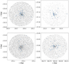 |
Fig. 1 Distribution in α and δ for GCs NGC 6304 (top left), NGC 6256 (top right), NGC 6553 (bottom left), and NGC 6401 (bottom right). The blue dots represent the stars found as overdensities with OCfinder, while grey dots are all stars in a cone search around the GC centre. |
4.2 New UBC clusters
After crossmatching our findings with known cluster catalogues, we were able to report 628 new OC candidates, which are numbered from UBC 1001 in order to differentiate from the UBC clusters found in Gaia DR2. These candidates were further divided into class A, class B, and class C based on a visual inspection of their distributions in (α, δ,  ,
,  , µδ) and their CMDs, aided with the distribution of radial velocities when available. We classify 566 OC candidates as class A (90% of the total), 26 (4%) as class B, and 36 (6%) as class C. Candidates in class A usually show a clustered distribution in the five astrometric dimensions and a clear sequence in the CMD. On the other hand, we generally classified candidates into class B if the main sequence formed by the candidate member stars in the CMD is truncated before G = 18 mag, and into class C if they also contain less than 15 members (where we consider the validation to be less reliable due to small numbers). In Fig. 2 we show examples of class A (two first rows), class B (third row), and class C (fourth row) OC candidates, which give a visual idea of the features of OC candidates in each of the classes.
A sample of the list of the new OC candidates, divided in their classes, can be found in Table 1. It contains the mean astro-metric parameters (i, δ, l, b,  ,
,  , µδ) and their dispersions for each OC candidate together with radial velocities when available. It also contains the apparent angular radius (θ) of the OC candidate, computed as the quadratic sum of σl and σb. A distance estimation computed from the CMD and mean parallax (see Sect. 4.2.2) is also provided, together with an estimation of age and line-of-sight extinction (Av). Finally, the number of stars considered as members, and member stars with available radial velocities, are also reported. We flagged the candidates that are positionally crossmatched to Kharchenko et al. (2013) (see Sect. 4.1). The full version of Table 1 can be found online at the CDS, together with Table 2 reporting the membership lists that resulted from our OCfinder method.
4.2.1 Characteristics of the new OC candidates
A small subset of the Gaia EDR3 stars have radial velocity measurements from Gaia DR2. We did not use these radial velocities in the clustering process; however, when available, they are useful to assess the reliability of the classification of the OC candidate. For the OC candidates in class A, 178 of them have radial velocity measurements, of which 72 are based on more than one star, and 25 are based on more than two stars. From these 25 OC candidates with radial velocities averaged over more than two stars, the median value of the radial velocity dispersions is 2.31 km s−1 with a median absolute dispersion of 2.03 km s−1, and 17 of them have radial velocity dispersions of 3 km s−1 at most. For class B and class C candidates, only four and six clusters have a mean radial velocity available, respectively, with 1 OC with more than two stars with radial velocity measurements in both cases. In these OCs, the radial velocity dispersions are 13.34 and 15.03 km s−1, respectively.
Figure 3 shows the distribution of the new OC candidates in Galactic l and b coordinates. We see that the location of the new candidates matches that of the known OCs. Even if the search is performed up to |b| ≤ 20°, new OCs are preferentially located within the Galactic disc at low latitudes. The vast majority of the new OC candidates (~99%) are located at |b| ≤ 10° (with only UBC 1186 and UBC 1530 with |b| > 10°, both belonging to class A), and ~93% of them within |b| ≤ 5°. We are also able to confirm some structures seen in previous studies, such as the lack of OCs in a region near l ~ 140° previously dubbed the Gulf of Camelopardalis (Cantat-Gaudin et al. 2019; Castro-Ginard et al. 2019).
The fact that our new detections are generally at larger distances can be seen in Fig. 4, where we show a histogram of the OC mean parallaxes for both the known population (Cantat-Gaudin et al. 2020) and new OC candidates. We see that the parallax distribution of the new OCs is positively skewed with respect to the distribution of known OC, meaning that the mode is slightly towards smaller mean parallaxes. Also, the drop in the distribution towards larger parallaxes is steeper in the new OCs’ distribution, showing the increasing difficulty in finding new nearby ones. In fact, only three OC candidates (0.60%) are closer than 1 kpc (see Sect. 4.2.4), and 75 (11.3%) are located within 1 and 2 kpc, probably due to a better completeness of previous surveys in these regions among other methodological effects. The relative parallax errors  for our new OCs range from 0.003 to 0.05 in the case of class A OCs and from 0.002 to 0.02 for class B and class C.
The heliocentric distances for the new OC candidates range from 860 pc to 9.6 kpc, computed from the distance modulus (see Sect. 4.2.2). In Fig. 5 we show the distribution in the X⊙ and Y⊙ coordinates, where we see that very few new OC candidates are detected within 1.5 kpc. This may be due to the combination of the following: (i) the approach adopted in OCfinder, where we are limited to the most compact object in the search region (see Sect. 3.2), and those are more likely to be already known at these close distances; and (ii) we expanded the search to G = 18 mag, which naturally pushes the search to farther distances (see Anders et al. 2021, to see the performance of OCfinder in terms of completeness for nearby objects), together with the above consideration of a better completeness of the nearby population.
The effect of the improvements in the Gaia EDR3 data is also seen in Fig. 6. There, we show a contour plot of the total proper motion dispersion as a function of the mean parallax, mimicking Fig. 1 in Cantat-Gaudin & Anders (2020). The densest part of the distribution, where most of the clusters are, is moved towards smaller σµ showing the huge improvement in the proper motion determinations (the effect is smaller in the parallax). This results in OCs being more compact (in proper motion and parallax), and thus it is easier to detect them as overdensities with respect to Gaia DR2.
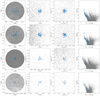 |
Fig. 2 Examples of the detected OCs for the different classes. The blue dots represent the detected member stars for each OC, while the grey dots are field stars queried in the Gaia archive using a cone search within 10 pc radius at the distance of the OC. From left to right, different panels represent: (i) positional distribution in α, δ, (ii) |


Some examples of the OCs found in this paper.
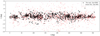 |
Fig. 3 Distribution of the OC population in l, b Galactic coordinates. Red triangles represent the OCs known prior to this study, reported in Cantat−Gaudin et al. (2020). Black crosses represent the new OCs found in this work using Gaia EDR3. |
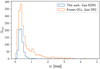 |
Fig. 4 Histogram of parallaxes for the OC population. The orange line shows the known population in Cantat-Gaudin et al. (2020), while the blue line shows the new findings in this study. |
4.2.2 Ages, distances, and line-of-sight extinctions
Cantat-Gaudin et al. (2020) trained an ANN on a set of well-characterised OCs with reliable estimations for ages, distances, and line-of-sight extinctions to estimate these parameters for almost the whole OC population characterised with Gaia DR2 data. We fine-tuned this ANN to estimate these astrophysical parameters for the newly discovered OCs with Gaia EDR3 data and we include them in our Table 1. The ANN takes the CMD of the OC member stars into account, together with the mean parallax plus two other quantities derived from the CMD to aid in the estimation (see Sect. 3.1 from Cantat-Gaudin et al. 2020, for details). For each OC, the ANN estimates its age, absorption (Av), and the distance modulus, and from this we were able to estimate the distance. The authors compared the values from a set of reference clusters with their estimated values to account for their uncertainties. They report that the uncertainties on the determination of the log age range from 0.15 to 0.25 dex for young OCs (≤8.5 dex), and from 0.1 to 0.2 dex for old OCs. In the case of extinction and distance modulus, the reported typical uncertainties range from 0.1 to 0.2 mag for Av, and from 0.1 to 0.2 mag in the distance modulus which corresponds to a 5% to 10% distance uncertainty. For further details, readers can refer to Sect. 3.4 from Cantat-Gaudin et al. (2020).
In Fig. 7 we plotted the distribution of the new OCs (crosses), together with the previously known population (triangles), in the Galactic disc for different age intervals: (i) younger than 100 Myr counting with 276 and 703 new and previously known OCs, respectively; (ii) from 100 to 500 Myr, with 248 new OCs and 675 previously known OCs; (iii) 500 Myr to 1 Gyr, 58 new OCs and 229 previously known OCs; and (iv) older than 1 Gyr, with 46 new OCs and 260 previously known OCs. These OCs are also colour-coded by their age. In the younger age bin (≤ 100 Myr), we find clear overdensities of OCs, which are following the different spiral arms (as fitted by Castro-Ginard et al. 2021). In the following age intervals, the distribution of the OCs is more dispersed, not showing significant overdensities, as expected.
The consistency of the age estimations with the previously known OC population is also shown in Fig. 8, where we show the distribution of the new OCs in the galactocentric radius (RGC) and altitude above the Galactic plane (Z) coordinates. We did not find young open clusters at high |Z| in the inner disc, but old OCs. The black circles highlight the OCs identified as old and with high |Z|, and specific plots for those are shown in show Fig. 9. These are interesting OCs, all of them are older than 1 Gyr and up to 4 Gyr (which is the oldest OC in our findings), and follow-up studies will be needed to explore their nature. At large RGC, we are also able to see the flare of the Galactic disc already seen with the OC population after Gaia DR2 Cantat-Gaudin et al. (2020). The extinction values range from 0.14 to 4.65 mag, with a distribution that is shown in Fig. 10.
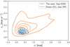 |
Fig. 6 Total proper motion dispersion |

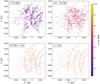 |
Fig. 7 Distribution of the new (crosses) and known (triangles, Cantat-Gaudin et al. 2020) OCs in the X⊙ versus Y⊙ coordinates for different age bins: 0−100 Myr (top left), 100–500 Myr (top right), 500 Myr –1 Gyr (bottom left), and more than 1 Gyr (bottom right). The dotted lines show the spiral arms as described by Castro-Ginard et al. (2021). |
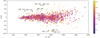 |
Fig. 8 Distribution of the newly found (crosses) and known (triangles) OCs in the RGC and Z coordinates, colour-coded by age. The black circles represent the selected OC shown in Fig. 9. |
4.2.3 Comments on UBC 1061
In Paper III, we reported the discovery of UBC 274, an old OC with an extended profile due to disruption by tidal forces. Here, we were also able to detect stellar groups that are probably undergoing disruption processes. This is the case for UBC 1061, which is a new OC found at l = 52.75° and b = −3.82°. It is located at a galactocentric distance of RGC = 6.77 kpc, associated with the Sagittarius arm (Reid et al. 2014; Castro-Ginard et al. 2021), and at Z = −247.95 pc. We estimate the age of UBC 1061 to be 1.3 Gyr, with an extinction value of Av = 0.74 mag. Figure 11 shows the distribution of its member stars in five astrometrical dimensions, in addition to its CMD where two blue straggler star candidates can be seen. While in parallax and proper motion UBC 1061 shows a clustered structure, it presents an elongation in the sky position diagram along the l coordinate, probably because it is undergoing disruption processes by the tidal forces (see Röser et al. 2019; Piatti 2020, for more examples). Such an old OC is rare in current OC catalogues, fewer than 20% of the reported OCs are older than 1 Gyr, and this is particularly the case for an inner disc cluster where young OCs are more frequent (Cantat-Gaudin et al. 2020). None of the 79 identified member stars of UBC 1061 have radial velocities in Gaia EDR3, and its red clump stars (at G ~ 14 mag) are at the faint limit for the GRVS sample. Therefore, UBC 1061 is an interesting case to follow up with on-ground spectroscopic surveys.
4.2.4 Candidates within 1 kpc
We found three OC candidates within 1 kpc from the Sun, where the OC census was assumed to be complete before Gaia. These OC candidates are UBC 1187, UBC 1573, and UBC 1592, which are located at 861, 862, and 977 pc, respectively, and all of them have angular sizes ≤0.10°. They are young objects, with none of them showing red clump stars in their CMDs, and they are poorly populated, with ~15 stars per cluster. This confirms the assumption that our methodology OCfinder is better suited to find objects with small angular sizes, and thus farther objects. However, since nearby objects are still detected, this opens the possibility of performing dedicated searches in the Solar neighbourhood which will be enhanced with the future Gaia DR3 thanks to the ~33 × 106 stars with radial velocity measurements6.
5 Conclusions
We report the detection of 628 new OCs within de Galactic disc, as the result of the adaptation and application of the OCfinder method to Gaia EDR3. For all of the new OCs, we report mean astrometric values (α, δ, l, b,  ,
,  , µδ) and radial velocity when available. We also estimate their ages, distances, and line-of-sight extinctions using an ANN trained on well-characterised OCs that was successfully applied to the OCs known in Gaia DR2. We divided the new OCs into class A, class B, and class C depending on the reliability of the candidate by inspecting the distribution of their member stars in all the available dimensions.
We find that the new OCs are located, in general, at farther distances than the clusters known from Gaia DR2. In fact, we were only able to detect three new objects closer than 1 kpc from the Sun. This is thanks to the improvements in parallax and proper motion precisions of Gaia EDR3, with respect to DR2 which allowed us to find more clustered objects (and thus we were able to search farther), and better knowledge of the OC population at close distances.
The estimation of astrophysical parameters also adds reliability to the OCs found with OCfinder. We see that young OCs follow the Galactic spiral arms, and they disperse on the Galactic disc as we explore older ages. Also, we find most OCs to be located at low |Z| in the inner disc, with the exception of some old (>1 Gyr) newly found OCs. In the outer disc, we are able to see the flaring of the Galactic disc with young OCs.
The use of a big data environment in the OCfinder methodology is key for a successful search of OCs. So far, 1274 OCs have been discovered using the OCfinder method, which represents almost 50% of the currently known OCs population. We have shown that improvements in the OCs census, both in terms of new detections or characterisation of known OCs, need to be aided by machine-learning methods to extract knowledge of the huge volume of high-quality data that is provided by Gaia EDR3. Future Gaia releases, as well as future photometric and spectroscopic Galactic surveys, will only increase this huge volume of high-quality data and thus the need for machine-learning methods.
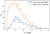 |
Fig. 10 Av histogram for the known (orange) and the new OC (blue) population. |
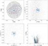 |
Fig. 11 Diagrams for UBC 1061. The blue dots are the stars selected as members with our OCfinder method, while the grey dots are field stars around 15 pc from the cluster centre. The diagrams correspond to the sky distribution, with density contour plots (top left), |


Acknowledgements
This work has made use of results from the European Space Agency (ESA) space mission Gaia, the data from which were processed by the Gaia Data Processing and Analysis Consortium (DPAC). Funding for the DPAC has been provided by national institutions, in particular the institutions participating in the Gaia Multilateral Agreement. The Gaia mission website is https://www.cosmos.esa.int/web/gaia. The authors are current or past members of the ESA Gaia mission team and of the Gaia DPAC. This work was (partially) funded by the Spanish MICIN/AEI/10.13039/501100011033 and by “ERDF A way of making Europe” by the “European Union” through grant RTI2018-095076-B-C21, and the Institute of Cosmos Sciences University of Barcelona (ICCUB, Unidad de Excelencia ‘María de Maeztu’) through grant CEX2019-000918-M. A.C.G. acknowledges Spanish Ministry FPI fellowship n. BES-2016-078499. This work has been partially supported by the Spanish Government (PID2019-107255GB), by Generalitat de Catalunya (contract 2014-SGR-1051). This research has made use of the VizieR catalogue access tool, CDS, Strasbourg, France. The original description of the VizieR service was published in A&AS 143, 23. This research has made extensive use of the TOPCAT software (Taylor 2005).
Appendix A Fitting magnitude uncertainties in Gaia EDR3
The Gaia EDR3 photometric error model used in this work is based on some relatively simple analytical functions derived fitting magnitude uncertainties for one million random sources in the Gaia EDR3 catalogue, covering all magnitude ranges. This error model was used to produce mock Gaia CMDs of the synthetic clusters used in the training of the ANN, described in Sect. 3.3.
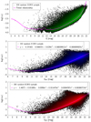 |
Fig. A.1 Gaia EDR3 magnitude uncertainties for G (top), GBP (centre), and GRP (bottom) and the fitted laws included in Tables A.1. |
In order to fit the uncertainties, we assumed a polynomial relationship between the logarithm of the Gaia EDR3 magnitude uncertainties,  , and their magnitudes, following the expression
 (A.1)
(A.1)
with GXP being either G, GBP, or GRP in every case. The resulting coefficients derived are shown in Table A.1.
For the G case, in some magnitude ranges the uncertainties in Gaia EDR3 show some complicated features due to calibration issues (see Riello et al. 2021), which cannot be fitted with a simple polynomial. A Gaussian function (Eq. A.2) was used instead of the polynomial (Eq. A.1) in these ranges:
 (A.2)
(A.2)
The actual fit used the following equation obtained taking the natural logarithm of Eq. A.2:
![Mathematical equation: ${\rm{ln}}\left[{\log \left({{\sigma_G}} \right) + 4} \right] = P \cdot {G^2} + Q \cdot G + R$](/articles/aa/full_html/2022/05/aa42568-21/aa42568-21-eq34.png) (A.3)
(A.3)
where we added 4 to log(σG) in order to avoid negative values when deriving its neperian logarithm. In order to retrieve the coefficients in Eq. A.2 from the fitted coefficients (Table A.1), the following transformation can be done from the values of P, Q, and R:
 (A.4)
(A.4)
 (A.5)
(A.5)
 (A.6)
(A.6)
In order to improve the behaviour of the obtained predictions, for all fitted passbands, we restricted our fitting to the median of the observations as a function of the magnitude, and not considering the individual observations of all sources used to derive these medians. Table A.1 shows the G magnitude intervals and the corresponding coefficients for the different fitted laws. The resulting fitted laws in Table A.1 are plotted in Fig. A.1.
References
- Alvarez Cid-Fuentes, J., Sola, S., Alvarez, P., Castro-Ginard, A., & Badia, R. 2019, in Proceedings of the 15th International Conference of eScience, 96 [Google Scholar]
- Anders, F., Cantat-Gaudin, T., Quadrino-Lodoso, I., et al. 2021, A&A, 645, L2 [NASA ADS] [CrossRef] [EDP Sciences] [Google Scholar]
- Bossini, D., Vallenari, A., Bragaglia, A., et al. 2019, A&A, 623, A108 [NASA ADS] [CrossRef] [EDP Sciences] [Google Scholar]
- Bressan, A., Marigo, P., Girardi, L., et al. 2012, MNRAS, 427, 127 [NASA ADS] [CrossRef] [Google Scholar]
- Campello, R.J.G.B., Moulavi, D., & Sander, J. 2013, in Advances in Knowledge Discovery and Data Mining, eds. J. Pei, V.S. Tseng, L. Cao, H. Motoda, & G. Xu (Berlin, Heidelberg: Springer), 160 [Google Scholar]
- Cantat-Gaudin, T., & Anders, F. 2020, A&A, 633, A99 [NASA ADS] [CrossRef] [EDP Sciences] [Google Scholar]
- Cantat-Gaudin, T., Jordi, C., Vallenari, A., et al. 2018, A&A, 618, A93 [NASA ADS] [CrossRef] [EDP Sciences] [Google Scholar]
- Cantat-Gaudin, T., Krone-Martins, A., Sedaghat, N., et al. 2019, A&A, 624, A126 [NASA ADS] [CrossRef] [EDP Sciences] [Google Scholar]
- Cantat-Gaudin, T., Anders, F., Castro-Ginard, A., et al. 2020, A&A, 640, A1 [NASA ADS] [CrossRef] [EDP Sciences] [Google Scholar]
- Carrera, R., Bragaglia, A., Cantat-Gaudin, T., et al. 2019, A&A, 623, A80 [NASA ADS] [CrossRef] [EDP Sciences] [Google Scholar]
- Carrera, R., Casamiquela, L., Carbajo-Hijarrubia, J., et al. 2022, A&A, 658, A14 [NASA ADS] [CrossRef] [EDP Sciences] [Google Scholar]
- Casamiquela, L., Castro-Ginard, A., Anders, F., & Soubiran, C. 2021a, A&A, 654, A151 [NASA ADS] [CrossRef] [EDP Sciences] [Google Scholar]
- Casamiquela, L., Soubiran, C., Jofré, P., et al. 2021b, A&A, 652, A25 [NASA ADS] [CrossRef] [EDP Sciences] [Google Scholar]
- Castro-Ginard, A., Jordi, C., Luri, X., et al. 2018, A&A, 618, A59 [NASA ADS] [CrossRef] [EDP Sciences] [Google Scholar]
- Castro-Ginard, A., Jordi, C., Luri, X., Cantat-Gaudin, T., & Balaguer-Nuñez, L. 2019, A&A, 627, A35 [NASA ADS] [CrossRef] [EDP Sciences] [Google Scholar]
- Castro-Ginard, A., Jordi, C., Luri, X., et al. 2020, A&A, 635, A45 [NASA ADS] [CrossRef] [EDP Sciences] [Google Scholar]
- Castro-Ginard, A., McMillan, P.J., Luri, X., et al. 2021, A&A, 652, A162 [NASA ADS] [CrossRef] [EDP Sciences] [Google Scholar]
- Colombo, D., Duarte-Cabral, A., Pettitt, A.R., et al. 2022, A&A, 658, A54 [NASA ADS] [CrossRef] [EDP Sciences] [Google Scholar]
- Dias, W.S., & Lépine, J.R.D. 2005, ApJ, 629, 825 [NASA ADS] [CrossRef] [Google Scholar]
- Dias, W.S., Alessi, B.S., Moitinho, A., & Lépine, J.R.D. 2002, A&A, 389, 871 [NASA ADS] [CrossRef] [EDP Sciences] [Google Scholar]
- Dias, W.S., Monteiro, H., Moitinho, A., et al. 2021, MNRAS, 504, 356 [NASA ADS] [CrossRef] [Google Scholar]
- Ester, M., Kriegel, H.-P., Sander, J., & Xu, X. 1996, in Proceedings of the Second International Conference on Knowledge Discovery and Data Mining, KDD'96 (AAAI Press), 226 [Google Scholar]
- Ferreira, F.A., Corradi, W.J.B., Maia, F.F.S., Angelo, M.S., & Santos, J.F.C., J. 2020, MNRAS, 496, 2021 [NASA ADS] [CrossRef] [Google Scholar]
- Gaia Collaboration (Brown, A.G.A., et al.) 2016, A&A, 595, A2 [NASA ADS] [CrossRef] [EDP Sciences] [Google Scholar]
- Gaia Collaboration (Brown, A.G.A., et al.) 2018, A&A, 616, A1 [NASA ADS] [CrossRef] [EDP Sciences] [Google Scholar]
- Gaia Collaboration (Brown, A.G.A., et al.) 2021, A&A, 649, A1 [NASA ADS] [CrossRef] [EDP Sciences] [Google Scholar]
- Hinton, G. 1989, Artif. Intell., 40, 185 [CrossRef] [Google Scholar]
- Hunt, E.L., & Reffert, S. 2021, A&A, 646, A104 [NASA ADS] [CrossRef] [EDP Sciences] [Google Scholar]
- Jaehnig, K., Bird, J., & Holley-Bockelmann, K. 2021, ApJ, 923, 129 [NASA ADS] [CrossRef] [Google Scholar]
- Kharchenko, N.V., Piskunov, A.E., Schilbach, E., Röser, S., & Scholz, R.-D. 2013, A&A, 558, A53 [NASA ADS] [CrossRef] [EDP Sciences] [Google Scholar]
- Lindegren, L., Hernandez, J., Bombrun, A., et al. 2018, A&A, 616, A2 [NASA ADS] [CrossRef] [EDP Sciences] [Google Scholar]
- Lindegren, L., Klioner, S.A., Hernandez, J., et al. 2021, A&A, 649, A2 [NASA ADS] [CrossRef] [EDP Sciences] [Google Scholar]
- Liu, L., & Pang, X. 2019, ApJS, 245, 32 [NASA ADS] [CrossRef] [Google Scholar]
- Luri, X., Palmer, M., Arenou, F., et al. 2014, A&A, 566, A119 [NASA ADS] [CrossRef] [EDP Sciences] [Google Scholar]
- Michalik, D., Lindegren, L., & Hobbs, D. 2015, A&A, 574, A115 [NASA ADS] [CrossRef] [EDP Sciences] [Google Scholar]
- Minniti, J.H., Zoccali, M., Rojas-Arriagada, A., et al. 2021, A&A, 654, A138 [NASA ADS] [CrossRef] [EDP Sciences] [Google Scholar]
- Monteiro, H., Dias, W.S., Moitinho, A., et al. 2020, MNRAS, 499, 1874 [NASA ADS] [CrossRef] [Google Scholar]
- Monteiro, H., Barros, D.A., Dias, W.S., & Lépine, J.R.D. 2021, Front. Astron. Space Sci., 8, 62 [NASA ADS] [CrossRef] [Google Scholar]
- NVIDIA, Vingelmann, P., & Fitzek, F.H. 2020, CUDA, release: 10.2.89 https://developer.nvidia.com/cuda-toolkit [Google Scholar]
- Paszke, A., Gross, S., Massa, F., et al. 2019, in Advances in Neural Information Processing Systems 32, eds. H. Wallach, H. Larochelle, A. Beygelzimer, et al., 8024 [Google Scholar]
- Pedregosa, F., Varoquaux, G., Gramfort, A., et al. 2011, J. Mach. Learn. Res., 12, 2825 [Google Scholar]
- Piatti, A.E. 2020, A&A, 639, A55 [NASA ADS] [CrossRef] [EDP Sciences] [Google Scholar]
- Reid, M.J., Menten, K.M., Brunthaler, A., et al. 2014, ApJ, 783, 130 [NASA ADS] [CrossRef] [Google Scholar]
- Riello, M., De Angeli, F., Evans, D.W., et al. 2021, A&A, 649, A3 [NASA ADS] [CrossRef] [EDP Sciences] [Google Scholar]
- Robin, A.C., Luri, X., Reylé, C., et al. 2012, A&A, 543, A100 [NASA ADS] [CrossRef] [EDP Sciences] [Google Scholar]
- Röser, S., Schilbach, E., & Goldman, B. 2019, A&A, 621, L2 [NASA ADS] [CrossRef] [EDP Sciences] [Google Scholar]
- Sim, G., Lee, S.H., Ann, H.B., & Kim, S. 2019, J. Korean Astron. Soc., 52, 145 [NASA ADS] [Google Scholar]
- Soubiran, C., Cantat-Gaudin, T., Romero-Gómez, M., et al. 2018, A&A, 619, A155 [NASA ADS] [CrossRef] [EDP Sciences] [Google Scholar]
- Spina, L., Ting, Y.S., De Silva, G.M., et al. 2021, MNRAS, 503, 3279 [CrossRef] [Google Scholar]
- Tarricq, Y., Soubiran, C., Casamiquela, L., et al. 2021, A&A, 647, A19 [NASA ADS] [CrossRef] [EDP Sciences] [Google Scholar]
- Taylor, M.B. 2005, ASP Conf. Ser 347, 29 [NASA ADS] [Google Scholar]
- Tejedor, E., Becerra, Y., Alomar, G., et al. 2017, Int. J. High Performance Comput. Appl., 31, 66 [CrossRef] [Google Scholar]
- Vasiliev, E., & Baumgardt, H. 2021, MNRAS, 505, 5978 [NASA ADS] [CrossRef] [Google Scholar]
GUMS (true values of instrinsic simulated sources) and GOG (observed attributes with simulated observational uncertainties) can be found in the Gaia archive: https://gea.esac.esa.int/archive/
Computed with the prescription given in https://github.com/agabrown/PyGaia
All Tables
All Figures
|
Fig. 1 Distribution in α and δ for GCs NGC 6304 (top left), NGC 6256 (top right), NGC 6553 (bottom left), and NGC 6401 (bottom right). The blue dots represent the stars found as overdensities with OCfinder, while grey dots are all stars in a cone search around the GC centre. |
| In the text | |
|
Fig. 2 Examples of the detected OCs for the different classes. The blue dots represent the detected member stars for each OC, while the grey dots are field stars queried in the Gaia archive using a cone search within 10 pc radius at the distance of the OC. From left to right, different panels represent: (i) positional distribution in α, δ, (ii) |
| In the text | |
|
Fig. 3 Distribution of the OC population in l, b Galactic coordinates. Red triangles represent the OCs known prior to this study, reported in Cantat−Gaudin et al. (2020). Black crosses represent the new OCs found in this work using Gaia EDR3. |
| In the text | |
|
Fig. 4 Histogram of parallaxes for the OC population. The orange line shows the known population in Cantat-Gaudin et al. (2020), while the blue line shows the new findings in this study. |
| In the text | |
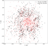 |
Fig. 5 Distribution in X⊙ and Y⊙ heliocentric coordinates. Symbols are the same as in Fig. 3. |
| In the text | |
|
Fig. 6 Total proper motion dispersion |
| In the text | |
|
Fig. 7 Distribution of the new (crosses) and known (triangles, Cantat-Gaudin et al. 2020) OCs in the X⊙ versus Y⊙ coordinates for different age bins: 0−100 Myr (top left), 100–500 Myr (top right), 500 Myr –1 Gyr (bottom left), and more than 1 Gyr (bottom right). The dotted lines show the spiral arms as described by Castro-Ginard et al. (2021). |
| In the text | |
|
Fig. 8 Distribution of the newly found (crosses) and known (triangles) OCs in the RGC and Z coordinates, colour-coded by age. The black circles represent the selected OC shown in Fig. 9. |
| In the text | |
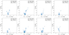 |
Fig. 9 CMDs of the high |Z| OCs, selected in Fig. 8. |
| In the text | |
|
Fig. 10 Av histogram for the known (orange) and the new OC (blue) population. |
| In the text | |
|
Fig. 11 Diagrams for UBC 1061. The blue dots are the stars selected as members with our OCfinder method, while the grey dots are field stars around 15 pc from the cluster centre. The diagrams correspond to the sky distribution, with density contour plots (top left), |
| In the text | |
|
Fig. A.1 Gaia EDR3 magnitude uncertainties for G (top), GBP (centre), and GRP (bottom) and the fitted laws included in Tables A.1. |
| In the text | |
Current usage metrics show cumulative count of Article Views (full-text article views including HTML views, PDF and ePub downloads, according to the available data) and Abstracts Views on Vision4Press platform.
Data correspond to usage on the plateform after 2015. The current usage metrics is available 48-96 hours after online publication and is updated daily on week days.
Initial download of the metrics may take a while.