| Issue |
A&A
Volume 661, May 2022
The Early Data Release of eROSITA and Mikhail Pavlinsky ART-XC on the SRG mission
|
|
|---|---|---|
| Article Number | A26 | |
| Number of page(s) | 11 | |
| Section | Cosmology (including clusters of galaxies) | |
| DOI | https://doi.org/10.1051/0004-6361/202141411 | |
| Published online | 18 May 2022 | |
eROSITA spectro-imaging analysis of the Abell 3408 galaxy cluster
1
Argelander-Institut für Astronomie (AIfA), Universität Bonn,
Auf dem Hügel 71,
53121
Bonn,
Germany
e-mail: This email address is being protected from spambots. You need JavaScript enabled to view it.
2
Max-Planck-Institut für extraterrestrische Physik,
Giessenbachstrasse 1,
85748
Garching,
Germany
Received:
28
May
2021
Accepted:
11
March
2022
Abstract
Context. The X-ray telescope eROSITA on board the newly launched Spectrum-Roentgen-Gamma (SRG) mission serendipitously observed the galaxy cluster Abell 3408 (A3408) during the performance verification observation of the active galactic nucleus 1H 0707–495. The field of view of eROSITA is one degree, which allowed us to trace the intriguing elongated morphology of the nearby (z = 0.0420) A3408 cluster. Despite its brightness (F500 ≈ 7 × 10⁻¹² ergs s−1 cm−2) and large extent (r200 ≈ 21'), it has not been observed by any modern X-ray observatory in over 20 yr. A neighboring cluster in the NW direction, A3407 (r200 ≈ 18', z = 0.0428), appears to be close at least in projection (~1.7 Mpc). This cluster pair might be in a pre- or post-merger state.
Aims. We aim to determine the detailed thermodynamical properties of this special cluster system for the first time. Furthermore, we aim to determine which of the previously suggested merger scenarios (pre- or post-merger) is preferred.
Methods. We performed a detailed X-ray spectro-imaging analysis of A3408. We constructed particle-background-subtracted and exposure-corrected images and surface brightness profiles in different sectors. The spectral analysis was performed out to 1.4r500 and included normalization, temperature, and metallicity profiles determined from elliptical annuli aligned with the elongation of A3408. Additionally, a temperature map is presented that depicts the distribution of the intracluster medium (ICM) temperature. Furthermore, we make use of data from the ROSAT all-sky survey to estimate some bulk properties of A3408 and A3407, using the growth-curve analysis method and scaling relations.
Results. The imaging analysis shows the complex morphology of A3408 with a strong elongation in the SE-NW direction. This is quantified by comparing the surface brightness profiles of the NW, SW, SE, and NE directions, where the NW and SE directions show a significantly higher surface brightness than the other directions. We determine a gas temperature kBr500 = (2.23 ± 0.09) keV in the range 0.2r500 to 0.5r500 from the spectral analysis. The temperature profile reveals a hot core within two arcminutes of the emission peak,  keV. Employing a mass–temperature relation, we obtain M500 = (9.27 ± 0.75) × 1013M⊙ iteratively. The r200 of A3407 and A3408 are found to overlap in projection, which makes ongoing interactions plausible. The two-dimensional temperature map reveals higher temperatures in the W than in the E direction.
Conclusions. The elliptical morphology together with the temperature distribution suggests that A3408 is an unrelaxed system. The system A3407 and A3408 is likely in a pre-merger state, with some interactions already affecting the ICM thermodynamical properties. In particular, increased temperatures in the direction of A3407 indicate adiabatic compression or shocks due to the starting interaction.
Key words: clusters: individual: Abell 3408 / galaxies: clusters: intracluster medium / X-rays: galaxies: clusters / intergalactic medium
© ESO 2022
1 Introduction
Galaxy clusters are the largest gravitationally bound systems in the Universe and are located at the nodes of the cosmic filaments. They form by merging processes of systems with lower masses and grow by accretion of matter along the filaments. The interactions between galaxy clusters are complex, that is, shock fronts caused by infalling subclusters or cold fronts with different origins can occur in the intracluster medium (ICM), as evidenced by X-ray spectro-imaging analyses (e.g., Markevitch & Vikhlinin 2007). Studying galaxy clusters and their interactions offers an insight into the large-scale structure of the Universe and its evolution. Bright, low-redshift, potentially interacting groups and clusters such as Abell 3408 (A3408, z = 0.0420; Struble & Rood 1999) and Abell 3407 (A3407, z = 0.0428; Struble & Rood 1999) provide the opportunity to widen this knowledge.
The extended ROentgen Survey with an Imaging Telescope Array (eROSITA) is a newly launched X-ray telescope (Predehl et al. 2021). It is the primary instrument of the German-Russian Spectrum-Roentgen-Gamma (SRG) mission (Sunyaev et al. 2021). SRG/eROSITA was launched on 13 July 2019 from Baikonur in Kazakhstan and is performing a deep survey of the entire X-ray sky since 8 December 2019. The main scientific purpose of the all-sky survey is to study galaxy clusters and their cosmic evolution (Merloni et al. 2012). Before the all-sky survey started, eROSITA went through a calibration and performance verification (CAL-PV) phase, in which the instrument carried out a series of observations of a variety of targets.
The galaxy cluster A3408 has been serendipitously observed during the PV observation of the active galactic nucleus (AGN) 1H 0707–495 (Boller et al. 2021). The field of view (FoV) of eROSITA of one degree allowed us to trace the intriguing elongated morphology of A3408. Despite its brightness and large extent, it has not been observed by any modern X-ray observatory in the past 20 yr. The discovery of an arc-like object (z = 0.073) in the optical band brought A3408 to the attention of the community (Campusano et al. 1998; Cypriano et al. 2001), as it was interpreted as an image of a background galaxy that is distorted due to the strong gravitational-lensing effect. The latest ICM temperature measurement was reported in Katayama et al. (2001), who measured a temperature of kBT = (2.9 ± 0.2) keV within a radius of 800 kpc, using data from the ASCA satellite. Chow-Martinez et al. (2014) classified A3408 and A3407 as a supercluster based on the small distance between the two neighboring clusters. Furthermore, there seems to be an indication that A3408 is interacting with A3407 (Nascimento et al. 2016). Based on a dynamical study of 122 member galaxies, Nascimento et al. concluded that A3408 and A3407 could be in a pre-merger scenario and might cross each other in less than ~ 1 h−1 Gyr, or they might be in a post-merger scenario and might have crossed each other ~1.65h−1 Gyr ago.
This article presents a detailed spectro-imaging analysis of A3408 with the main goal of describing the intriguing cluster morphology, temperature, and abundance distribution. Further-more, we search for indications of possible interactions between A3408 and A3407. The article is structured as follows: Sect. 2 contains the analysis of the ROSAT data of A3408 and A3407. Sections 3 and 4 describe the data processing of the eROSITA data and source detection, respectively. The eROSITA imaging analysis including results is presented in Sect. 5, and the spectral analysis is described in Sect. 6. The results are discussed in Sect. 7. Finally, Sect. 8 contains the conclusions and an outlook on further work. The applied cosmological model is a flat ACDM cosmology with Ωm = 0.3, ΩΛ = 0.7, and H0 = 70 km s−1 Mpc−1, with H0 = 100 h km s−1Mpc−1 and physical angular scales of 0.8289 kpcarcsec−1 at z = 0.0420 and 0.8439 kpcarcsec−1 at z = 0.0428.
2 ROSAT cluster properties
Both A3407 and A3408 show significant emission in the ROSAT all-sky survey maps. In order to obtain some insights into A3407, we estimated its properties from the hard-band images of the survey (0.5–2 keV), and applied the same methods to A3408 for consistency.
The process relies on the growth-curve analysis method developed by Böhringer et al. (2001), and our implementation is described in detail in Xu et al. (2018). It first estimates a local background from a large annulus around its center for each cluster (25′–45′). Then, it extracts an integrated background-subtracted count-rate profile out to 25′, in bins of 0.5′. In determining both the background and growth curve, we masked contaminating sources and corrected for the missing flux assuming azimuthal symmetry. At this stage, we measured a reference source count rate CRap within the significance radius, θap, defined as the aperture out of which an increase in total source count rate can no longer be detected. In a second part of the process, we sought to estimate cluster properties within, r500, the radius within which the average cluster density is 500 times higher than the critical density of the Universe at the cluster redshift z. For this, we relied on a set of scaling relations obtained from XMM-Newton follow-up observations of complete ROSAT-selected cluster samples. For a given cluster mass M500, the luminosity L500 in 0.1–2.4 keV was first computed from the Schellenberger & Reiprich (2017) relation, which relies on the HIFLUGCS sample (Reiprich & Böhringer 2002). It was then converted into a ROSAT count rate CR500, using for the spectral model a temperature derived from the Lovisari et al. (2015) M500 − TX relation, which is based on a subsample of the eeHI-FLUGCS clusters (Reiprich 2017). Both conversions ignore the scatter around the mean scaling relations. Using an iterative procedure, the algorithm identifies the unique set of cluster parameters whose predicted M500, r500, L500, TX, and CR500 correspond to the cluster photometric measurements (θap, CRap). The latter conversion assumes a β-model surface brightness with a fixed β = 2/3 and accounts for the redistribution arising from the ROSAT point spread function (PSF). For the required β-model core radius, we scaled it with r500 using the median relation observed in the HIFLUGCS sample, rc = 0.12 × r500, which provides an adequate model for the outskirts of most HIFLUGCS clusters (Schellenberger, priv. comm.).
Reiprich et al. (2013) reported that rvir(z = 0) ≈ r100 ≈ 1.36 r200 and r500 ≈ 0.65 r200. Using these relations, we estimated r200 and r100 of A3408 and A3407, respectively.
The results of the analysis of the ROSAT data of both clusters are summarized in Table 1. The center of A3407 was taken from the catalog in Abell et al. (1989). The distance between the cluster centers at redshift z = 0.042 is ~1.7 Mpc. The estimated r200 is (1.066 ± 0.048) Mpc for A3408 and (0.895 ± 0.049) Mpc for A3407. The r200 and r100 of both clusters overlap at least in projection, which means that interactions are plausible. All radii are illustrated in Sect. 6.
3 Data processing
The AGN 1H 0707–495 was observed by eROSITA on 11 October 2019 (Boller et al. 2021). The corresponding observation ID is 300003. This pointed PV observation was performed by telescope modules (TM) 1, 2, 5, 6, and 7. The observations by TM 1 and 2 did not reach the full exposure time of 50 ks. TM 3 and 4 were not active during the entire observation. All observation times are summarized in Table 2.
3.1 Data preparation
The data used in this work were obtained from processing configuration 001. The data reduction was performed using the eROSITA Science Analysis Software System (eSASS, Brunner et al. 2022), release 201009.
The event files were generated in the full energy band of 0.2–10.0 keV using the eSASS task evtool with parameters pattern=15 and flag=Sxc0Sfff30, that is, all single, double, triple, and quadruple patterns were selected and events located in the strongly vignetted corners of the square CCDs were removed because uncertainties in the vignetting and PSF calibration remained.
In general, the observation could be affected by a temporally varying background component, for instance, by soft proton flares as observed by XMM-Newton (e.g., Reiprich et al. 2004). In order to verify the data quality, light curves were created with the eSASS task flaregti in the 6.0–9.0 keV energy band. They were inspected for each TM. A flare was determined for TM 5 and 7. Consequently, a consistent filtering procedure was applied to all event files. The filtering procedure includes automatic and additional filtering. The automatic filtering results in good-time intervals (GTIs) from the standard eSASS processing. The additional filtering determines the 3σ interval by fitting a Gaussian to the histogram of the rates. Any interval beyond ±3σ was rejected from the data. Finally, the GTIs from the automatic and additional filtering were combined. These clean and filtered event files for each TM are used for the analysis in this work. The observation times after (and before) the filtering procedure are listed in Table 2, where the highest impact of ~9% can be seen for TM 7, a camera without on-chip optical light filters (see Sect. 3.2). More information about the filtering procedure and all light curves in the 6.0–9.0 keV energy band is shown in Appendix A.
PV observation (ObsID: 300003, SRG Observing mode: pointing) of the AGN 1H 0707–495 and the A3408 galaxy cluster on 11 October 2019 by eROSITA.
3.2 Light leak
During the camera commissioning period, light-leak contamination was detected in TM 5 and 7, that is, parts of the respective CCDs are contaminated by optical photons. These optical photons produce apparent X-ray events with energies below ~0.8 keV. TM 1–4 and 6 are equipped with on-chip optical light filters and are therefore not affected by the light leak (more details in Predehl et al. 2021). For this reason, the imaging and spectral analysis in this work applies different energy bands for TM with on-chip filters, that is, TM 1, 2 and 6, in contrast to TM without on-chip filters, that is, TM 5 and 7.
4 Source detection
The eSASS source detection algorithm (Brunner et al. 2022) detects point sources in the observation based on the sliding-cell method. We ran the corresponding eSASS tasks (erbox1) on the combined clean and filtered event files of TM 1, 2, 5, 6, and 7 in the 0.8–5.0 keV energy band.
First, the eSASS task erbox in local mode searched for signals that exceed a certain threshold and creates a catalog with detected sources. The significance of the enhancement is measured by the minimum detection likelihood, which is defined as the probability of one source being spurious (see Appendix A.5 in Brunner et al. 2022 for further details). We applied the default parameters likemin = 6 (detection likelihood threshold), nruns = 3 (number of image rebinning steps), and boxsize = 4 (detection box size).
In a next step, a background map was generated with the task erbackmap by masking out the previously detected sources and using an adaptive smoothing algorithm with a signal-to-noise ratio (S/N) of 40. Finally, erbox performs a second source detection in map mode with respect to the newly created background map. This step refines the source detection.
Finally, a maximum likelihood fitting method was applied on the new source catalog using the eSASS task ermldet. Each detected source was modeled using the eROSITA PSF and in our case, was folded with an extent model (beta model). Some of the model parameters include the source extent (in our case, given by the core radius of the beta model). The total number of detected sources in the 1 deg circular FoV (0.833 sq. deg) is 330, of which 318 are point-like sources, and 12 are extended sources (i.e., with an extent larger than zero).
The resulting catalog was then visually inspected to confirm that no point sources are missed. Using the final catalog, we excluded all the detected point sources and back- or foreground extended sources in the FoV from further analysis.
5 eROSITA imaging analysis
5.1 Preparation
The imaging analysis provides a first insight into the spatial distribution of the ICM emission of A3408. The particle background subtraction and the exposure correction were accomplished following the procedure described in Reiprich et al. (2021). With this method, an image was created in the 0.3–2.3 keV energy band for TM 1, 2, and 6 and in the 1.0–2.3 keV energy band for TM 5 and 7, ensuring they are not affected by the light leak. In the following, the combination of the two TM-dependent energy bands is referred to as the soft band. The image extraction for each TM was performed with the eSASS task evtool, while the corresponding vignetted and unvignetted exposure maps were generated with expmap.
In this procedure, the particle background is modeled using the eROSITA filter-wheel-closed (FWC) observation data. The spatial variation of the particle background was found to be very small and temporally stable (Freyberg et al. 2020). Within the procedure, a particle background map is created for each TM using the signal in the hard band (6.0–9.0 keV) as scaling. The spatial distribution is provided by multiplying to the respective unvignetted exposure maps. For this, we determined the hard counts Hobs in the observation data in the 6.0–9.0 keV energy band and the ratio R of the counts in the FWC data in the 0.3–2.3 keV energy band (1.0–2.3 keV for TM 5 and 7) and in the 6.0–9.0 keV energy band. The counts of the particle background in the 0.3–2.3 keV energy band (1.0–2.3 keV for TM 5 and 7) were estimated by multiplying the hard counts Hobs with the ratio R. This number, HobsR, was then multiplied to the unvignetted exposure map, which was normalized to unity by dividing each pixel by the sum of all the pixel values. These background maps were then subtracted from the respective individual photon images. This procedure was applied to the unsmoothed images. The resulting particle background-subtracted photon images for the individual TMs were aggregated, resulting in a combined particle background-subtracted soft-band photon image.
For the exposure correction, exposure maps were generated using expmap for each TM. The vignetting function was applied during this process. The exposure maps from TM 1, 2, and 6 were co-added, while those of the TMs affected by the light leak, that is, TM 5 and 7, were coadded separately. Then both coadded exposure maps were combined with proper scaling, as described in detail in Reiprich et al. (2021). In a last step, the particle background-subtracted image in the soft band was divided by the combined exposure map. The final particle background-subtracted and exposure- and vignetting-corrected soft-band image is shown in Fig. 1.
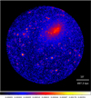 |
Fig. 1 Particle background-subtracted and exposure-corrected photon image of A3408 with TM 1, 2, 5, 6, and 7 in the soft band (0.3–2.3 keV energy band for TM 1, 2, and 6 and 1.0–2.3 keV energy band for TM 5 and 7) in logarithmic scale. |
5.2 Cluster center and general features
We applied an adaptive smoothing to the final soft-band image after refilling removed point sources across the FoV with the surrounding background surface brightness. For this purpose, we used the XMM-Newton Science Analysis System (SAS, 18.0.0) task asmooth2 with the parameter smoothstyle = adaptive, further specifying an S/N of 10, a minimum number of 10 pixels, and a maximum number of 20 pixels.
Figure 2 shows the resulting adaptively smoothed soft-band image of A3408. The image outlines the bright central region of A3408 and the elliptical appearance to the outer radii. The center is shifted NW relative to the larger-scale emission, where the emission peak is determined to be at RA = 107.0948 deg, Dec = −49.1933 deg. This peak was used as cluster center for all subsequent profile analyses. Furthermore, enhanced emission is visible in the W toward A3407 in the outermost regions.
The brightest cluster galaxy of A3408 is identified as 2MASX J07082956-4912505 at a redshift of z = 0.042 (Galli et al. 1993). This galaxy is located ~2′ SE of the emission peak. A slightly fainter galaxy at a similar redshift, 2MASX J07081135-4909525, is also located ~2′ from the cluster center, but in the opposite direction, that is, NW. Coincident with the positions of these two galaxies are two X-ray point sources. It is not clear whether the X-ray emission of these two galaxies is thermal or due to activity of their central supermassive black holes. An obvious but exciting possibility is that they were the brightest cluster galaxies of two previous clusters that merged. This would also fit well and explain the very elongated shape of the overall X-ray surface brightness distribution. This would imply that A3408 is not only in a likely pre-merger state with respect to A3407, but at the same time is in a post-merger state. This means that we may have caught this system in a quite active phase of its evolution.
Moreover, there are some extended emission regions, for example, E and S of A3408. The extended source to the east is probably a galaxy group that is infalling into the main system. The brightest cluster galaxy of this possibly infalling group is identified as 2MASS J07105737-4914161 at a redshift of z = 0.039 (Huchra et al. 2012). The general emission toward the east extends to beyond r200. The extended source to the south may also be an infalling clump, but no redshift estimate is available, therefore a projected background cluster cannot be excluded at present. However, there are three galaxies with redshift estimates within 10′, each located at similar redshifts as A3408, which is an indication that the southern extended source is indeed an infalling clump.
5.3 Surface brightness profile
The surface brightness profile enables us to study the morphology quantitatively by comparing different sectors. We define the surface brightness as the number of photons per detector area (which corresponds to the effective area of the combined telescope, filter, and detector system) per exposure time per area on the sky. We calculated the photon counts in a given region with funcnts from FUNTOOLS (1.4.7) on the particle background-subtracted photon image in the soft band. We verified that we obtained consistent results using only TM with on-chip filters (TM 1, 2, and 6) compared to the default image of TM 1, 2, 5, 6, and 7.
The surface brightness profile was calculated for four different sectors, NW, SW, SE, and NE, as shown in the left panel of Fig. 3, where the profile is centered at the cluster center determined in Sect. 5.2 and most emission is visible SE-NW along the elongation of A3408. In detail, circular annuli with a width of 20″ and a maximum outer radius of r200 were chosen to sum up the counts from the particle background-subtracted image and to determine the average from the exposure map. The surface brightness profile of the NW sector only contains bins that are at least 50% inside the FoV. In a next step, the source counts were divided by the average exposure in a given source area. Additionally, the X-ray fore- and background (CXB) counts were obtained from the area of r100 to the edge of the FoV and were subtracted from the source counts after exposure and area scaling. We obtained the error of each source region from funcnts (using the particle background-subtracted photon image). Then we also obtained the error from sky background region. The two errors (also from the exposure) were propagated to calculate the surface brightness profile. The resulting surface brightness profile for each sector is shown in Fig. 4. A comparison of all profiles shows an enhanced surface brightness in the NW in the central regions of ~1′ to ~3′. From there on, the surface brightness increases in the SE relative to the other directions, which confirms the elongation of A3408 in SE-NW direction. At outer radii (> 10′), all profiles become more consistent with each other, while there is still enhanced emission in the NW, as previously seen in the adaptively smoothed image. Out to r200, there is slightly more emission in the NE compared to the SE.
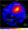 |
Fig. 2 Adaptively smoothed particle background-subtracted and exposure-corrected photon image in the soft band (0.3–2.3 keV energy band for TM 1, 2, and 6 and 1.0–2.3 keV energy band for TM 5 and 7) in logarithmic scale. There seems to be diffuse emission out to beyond r200 (dashed white line) in the western direction, including possibly infalling galaxy groups (“extended source”) in the east at a similar redshift as A3408 and south (no redshift estimate available). |
6 eROSITA spectral analysis
The extraction procedure of all spectra and response files was performed using the eSASS task srctool. It creates the spectrum files for selected source and background regions and also extracts the corresponding response matrices (RMFs) and effective areas (ARFs). The point sources detected in the image (see Sect. 4) were excluded from source and background regions throughout the spectral analysis.
The X-ray spectral fitting package XSPEC 12.10.1 was used for the spectral fitting (Arnaud 1996) applying the c stat likelihood for Poission statistics. The solar abundance table was taken from Asplund et al. (2009). The source spectra of all TM were modeled simultaneously with the background spectra and the instrumental background obtained from the FWC data of all TM. The 0.3–8.0 keV energy band was used for TM 1, 2, and 6, while the lower energy used in TM 5 and 7 was 1.0 keV to avoid the effects of optical light leak.
The cluster emission was modeled by an absorbed thermal apec model with ATOMDB version 3.0.9 (Foster et al. 2012) within XSPEC and the absorption model TBabs for Galactic absorption (Wilms et al. 2000). In the thermal apec model, the redshift ζ was frozen to 0.0420 (Struble & Rood 1999), while the cluster temperature T, metallicity Z, and normalization Κ were free to vary. The normalization Κ is defined as
![Mathematical equation: $K = {{{{10}^{- 14}}} \over {4\pi {{[{D_{\rm{A}}}(z + 1)]}^2}}}\int {{n_{\rm{e}}}{n_{\rm{H}}}dV.}$](/articles/aa/full_html/2022/05/aa41411-21/aa41411-21-eq2.png) (1)
(1)
DA is the angular diameter distance in units of cm, ne is the electron density and nH is the hydrogen density in units of cm−3. For the absorption model TBabs, we set the equivalent hydrogen column density NH to 6 × 10²⁰ atoms cm−2 (Willingale et al. 2013).
The observed background usually consists of the particle background and cosmic X-ray background (CXB). The particle background is produced by energetic particles that interact with the surrounding material or the detector itself. The CXB is composed of faint X-ray point sources that are unresolved by eROSITA. Furthermore, the local hot bubble (LHB) and the galactic halo (GH) also contribute to the CXB (Lumb et al. 2002; Kuntz & Snowden 2008; Gilli et al. 2006).
The particle background was estimated with eROSITA FWC observation data. The corresponding model contains Gaussian emission lines and power-law models with free normalizations. The normalization of the particle background has been found to vary only by ~6% (Reiprich et al. 2021). Fixing this background normalization during the fit to ±6% of its nominal value changes the resulting best-fit cluster parameters, that is, the temperature T, metallicity Z, and normalization K, only within 1σ.
The background spectra for the CXB model were extracted from a region starting at r200 of the cluster out to the edge of the FoV excluding point sources. The CXB model contains three components: An unabsorbed thermal apec model with a temperature of 0.099 keV for LHB (metallicity set to 1.0, redshift set to 0.0), an absorbed thermal model with a temperature of 0.225 keV (McCammon et al. 2002) for the GH (metallicity set to 1.0, red-shift frozen to 0.0), and an absorbed power law with a photon index of 1.41 (De Luca & Molendi 2004) for the unresolved point sources. In addition, we added an absorbed thermal apec model to account for residual cluster emission in the background region.
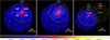 |
Fig. 3 Particle background-subtracted and exposure-corrected photon image of TM 1, 2, 5, 6, and 7 in the soft band in logarithmic scale. Left: four sectors, SW, SE, NW, and NE out to r200 (dashed white lines), are illustrated. These areas were used to extract the counts for the surface brightness profiles. Center: elliptical annuli (white) out to a semimajor axis of 19 and a semiminor axis of 9.5. The annuli have the same eccentricity and angle of 40 deg, which were chosen to be visually aligned to the cluster shape. These areas were used to obtain temperature, metallicity, and normalization profiles. Furthermore, the temperature map was determined within a circular area of 19 (magenta) to ensure enough counts in the source regions for spectral fitting. Right: calculated characteristic radii r500 (green), r200 (dashed white) and r100 (yellow) of A3408 and A3407 from analyzing ROSAT data and applying the relations r100 ≈ 1.36r200 and r500 ≈ 0.65r200 in Reiprich et al. (2013). |
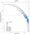 |
Fig. 4 Surface brightness profiles obtained in four different sectors (SW, SE, NW, and NE; as illustrated in Fig. 3, left). The CXB level is shown as the dashed orange line, and r500 and r200 are shown as dashed gray and black lines, respectively. |
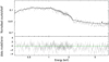 |
Fig. 5 eROSITA spectrum of TM 6 in 0.2r500 to 0.5r500 with corresponding model. |
6.1 eROSITA cluster properties
Cluster masses are not directly measurable. One way to determine them is through the use of scaling relations using X-ray observables. The M500 − T relation enables the calculation of the cluster mass M500 by the ICM temperature T.
In this procedure, the central region of A3408 was excluded to avoid emission from nongravitational heating and cooling processes in the cluster center, that is, the temperature is described by the depth of the gravitational potential (Lovisari et al. 2015). After extracting the spectra from an arbitrary annulus, the spectral fitting was performed as previously explained. Figure 5 illustrates the spectrum and model of TM 6. The mass estimation was then performed using the M500 − T relation
 (2)
(2)
from Lovisari et al. (2015), where  , c2 = 2 keV, a = (1.65 ± 0.07), b = (0.19 ± 0.02), and log(x) is base 10. Assuming spherical symmetry, the characteristic radius r500 can be derived from the estimated mass M500. We adopted a critical density of ρcrit = 9.567 × 10⁻²⁷ kg m−3 at the cluster redshift zA3408 = 0.0423. Comparing the calculated r500 with the source extraction area, we can iteratively find the temperature T and mass M500 within 0.2r500 to 0.5r500. Iterating this procedure for A3408 resulted in an ICM temperature of kBT = 2.23 ± 0.09 keV and metallicity of Z = 0.22 ± 0.03 Z⊙ within an annulus of 2.8′ to 7.3′, corresponding to 0.2r500 to 0.5r500, respectively, where r500 = (13.65 ± 0.37)′.
As described before, r200 and r100 can be estimated from r500. The results are listed in Table 3.
Furthermore, we performed spectral fitting within a radius of 800 kpc as used in Katayama et al. (2001) for a comparison with their results obtained from ASCA data. We find a best-fit temperature  keV and metallicity
  . However, Katayama et al. (2001) measured a temperature of
  keV and metallicity of
  , applying the single-temperature thermal emission model from Raymond & Smith (1977) in 0.7–10.0 keV, while redshift z and equivalent hydrogen column NH were equal to the values used in this work. One possible reason for this deviation is the multitemperature structure of the ICM. Gas might be present at different temperatures along the line of sight in the extraction area. When a single-temperature model is used to describe the spectra, the result depends on the observing telescope and its response. A higher sensitivity at lower energies would result in stronger weighting of the Fe L shell emission line complex, resulting in a lower temperature, while a telescope with a higher sensitivity at higher energies would lead to a higher temperature, as illustrated in detail in Reiprich et al. (2013), for instance. eROSITA has a larger effective area at lower X-ray energies than ASCA (Predehl et al. 2021; Tanaka et al. 1994), that is, the multitemperature structure could qualitatively explain the lower temperature obtained from eROSITA.
Estimated cluster properties of A3408 applying the M500 - T relation from Lovisari et al. (2015).
6.2 Temperature, metallicity, and normalization profiles
Since A3408 has an elongated morphology, the temperature, metallicity, and normalization profiles were obtained from elliptical annuli out to a semimajor axis of 19′ and a semiminor axis of 9.5′ to ensure enough source counts. The annuli have the same eccentricity and angle of 40 deg, chosen visually aligned to the cluster shape, as shown in the center panel of Fig. 3.
The spectral fitting was performed in the 0.3–8.0keV energy band for TM 1, 2, and 6, and 1.0–8.0 keV for TM 5 and 7, as explained previously. The resulting temperature, metallicity, and normalization profiles are presented in Fig. 6. We also performed spectral fitting of the NW half and SE half of the full elliptical annuli, subdivided along the semiminor axis. The temperatures of the five outer regions of the profile show an indication for a systematic trend: each of them is higher in the NW and lower in the SE direction at ~1σ significance compared to the results of the full annuli. For further investigations of these differences and the temperature distribution of A3408, it is useful to create a temperature map with more bins aligned to the cluster emission.
6.3 Temperature map
In order to create a temperature map of the A3408 cluster, the region outside 19′ was masked along with the point sources in the field, and the Sanders (2006) contour binning software was used to create a bin map of the cluster. The input parameters of the software determine the size and shape of the bins in the resulting bin map, where the distribution of the bins follows the surface brightness of the cluster. We applied the contour binning software to the combined image of TM 1, 2, 5, 6, and 7 in the soft band to create a bin map with a number of counts of 2500 per bin.
Following the binning of the data, masks of each bin were created and used as inputs for the eSASS task srctool to perform spectral extraction for each TM. The spectral fitting was performed as described in Sect. 6. The resulting best-fit temperature values and errors were then saved to the corresponding bin in the temperature map.
The resulting temperature map with corresponding relative errors for each bin is shown in Fig. 7. Due to the elliptical morphology, as described in the imaging analysis, the contour binning method creates bins aligned to the elongation of A3408. A few more cooler bins are visible in the SE than in the NW. Furthermore, the temperatures appear to be higher in the W than in the E. Relative errors are about 10–30%.
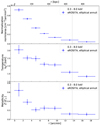 |
Fig. 6 Normalization (top), temperature (middle), and metallicity (bottom) profiles of A3408 using elliptical annuli, where r represents the semimajor axis. The dashed gray lines indicate r500 of the cluster. |
7 Discussion
The imaging analysis underlines the intriguing morphology of A3408, which is elongated in the SE–NW direction. This is confirmed quantitatively in the comparison of the surface brightness profiles of the four sectors NW, SW, SE, and NE. This indicates that A3408 is not a relaxed system. The ratio of the semimajor and semiminor axis is 2.0. The adaptively smoothed image shows enhanced emission toward A3407. In addition to this qualitative evidence, the surface brightness profile provides quantitative evidence of higher emission in the NW sector compared to the other regions. The comparison of the surface brightness profiles of the two sectors NW and SE is shown in Fig. 8. The relative differences between NW to SE are 60% for the prominent peak at 15.3′, 68% at 16.3′, and 79% at 17.0′, as listed in Table 4.
Nascimento et al. (2016) described a weak bridge connecting A3407 and A3408 in a ROSAT PSPC image. However, they also mentioned the gap introduced by the support structure of the PSPC entrance window, which could distort the appearance. Nevertheless, the overlapping at least in projection of r200 of the two clusters obtained from our ROSAT analysis of the two clusters supports the idea that A3407 and A3408 interact with each other. Hence, this cluster pair is another very good candidate for studying bridge emission in X-rays and radio, as in the systems A399/401 (e.g., Fujita et al. 2008; Ade et al. 2013; Govoni et al. 2019), A1758 (e.g., Botteon et al. 2020), A3391/95 (e.g., Reiprich et al. 2021; Brüggen et al. 2021), and A2029/2033 (e.g., Mirakhor et al. 2022), in order to understand hydrodynamical processes including the early onset of turbulence.
Furthermore, the cluster properties r200, r200, and r100 are consistent with the results of Nascimento et al. (2016). In their dynamical analysis of 122 member galaxies of A3407 and A3408, the authors found galaxy velocity dispersions of  and
and  and corresponding virial masses of
  and
and  . With these results and the assumption MV ≈ M100, the characteristic radii r100, r200, r500 can be estimated again with the scaling relations from Reiprich et al. (2013). We find r100 ≈ 33′, r200 ≈ 24′, and r500 ≈ 16′ for A3408, which is in agreement with the findings in this work. For A3407, we find r100 ≈ 42′, r200 ≈ 31′, and r500 ≈ 20′, which is significantly higher than the results from the analysis of the ROSAT data. However, velocity dispersions for close systems such as A3408 and A3407 might result in overestimated mass estimates. This might explain the discrepancy for A3407. From the X-ray images, that is, from the X-ray luminosities, it appears that is A3408 the more massive cluster, and not A3407, as reported by Nascimento et al. (2016).
A few lower temperatures are visible in the southern bins compared to the northern bins, but the west also seems to be hotter than the east. A3407 lies in the NW direction, therefore, this could indicate a shock front or adiabatically compressed gas due to onsetting interaction with A3407. Furthermore, in the temperature map and in the temperature profile, a hot core is discovered. How early interaction with A3407 could lead to a hot core in A3408 is not completely obvious; it might be the result of a recent previous merger that might also have contributed to forming the very elongated shape. Hot cores are typically found in non-cool-core clusters (as defined through the cooling time) and that non-cool-core clusters are predominantly found in merging or substructured clusters (e.g., Hudson et al. 2010). Therefore, a hot core is an indicator for recent merger activity.
The temperatures of the outer three bins (in 4′–12′) in the W (Tw,1, Tw,2 and Tw,3) and Ε (TE,1, Te,2, and TΕ,3) are listed in Table 5. The discrepancies of the temperatures are at 1σ for Tw,1 and ΤΈ,1, 1σ for TW,2 and TΕ,2, and 3σ for TW,3 and TΕ,3.
Surface brightness in the SE and NW sector.
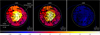 |
Fig. 7 Temperature map of A3408. The eROSITA FoV (blue) and r200 (dashed white line) are indicated. Left: temperature map with an additional annulus of 4–12 (black) for visualization. Center, temperature map with surface brightness contours generated from the particle background-subtracted and exposure-corrected soft-band image overlaid in black. Right: relative errors for each temperature in the corresponding bin. |
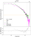 |
Fig. 8 Comparison of surface brightness profiles obtained in two sectors (SE and NW, as illustrated in the left panel of Fig. 3). The CXB level is shown as a dashed orange line, and r500 and r200 are shown as dashed gray and black lines, respectively. |
8 Conclusions
The galaxy cluster A3408 has been serendipitously observed during the eROSITA CAL-PV phase. The imaging analysis underlines the intriguing elliptical cluster morphology in the SE-NW direction. We determine for A3408 a gas temperature of kBT500 = (2.23 ± 0.09) keV within 0.2r500 to 0.5r500, a mass of M500 = (9.27 ± 0.75) × 1013Μ⊙, and r500 = (679 ± 18) kpc. There are indications that A3407 and A3408 are interacting, for instance, enhanced emission from A3408 toward A3407 in the adaptively smoothed image and the surface brightness profile, and enhanced temperatures in the NW direction of A3408. We interpret this such that the ICM thermodynamic properties of A3408 are affected by early interaction with the A3407 cluster.
The eROSITA All-Sky Survey (eRASS) will enable the analysis of the whole A3407–A3408 system. The cluster properties of A3407 together with this analysis will lead to a better understanding of this system. Furthermore, if an emission bridge does connect the two clusters, the eRASS image will provide its observation. More generally, given the early eROSITA results on cluster outskirts and infall regions (e.g., Reiprich et al. 2021; Ghirardini et al. 2021; Churazov et al. 2021; Veronica et al. 2021; Whelan et al. 2021; Sanders et al. 2022), and given the close correspondence to similar structures observed in cosmological hydrodynamical simulations (e.g., Biffi et al. 2022), we may expect that bridges and clumpy filaments will be discovered in several more nearby systems in the future in the eRASS. These systems can then be studied in detail after the eight surveys are completed using the SRG/eROSITA scanning mode, with which areas of tens of square degrees can be scanned efficiently, homogeneously, and deeply. Furthermore, when Athena (e.g., Nandra et al. 2013) operates in the 2030s, it will be able to characterize the density, temperature, and metallicity structure of the cluster outskirts and eROSITA-discovered emission filaments in great detail.
Temperature values of the outer bins within 4–12 in the east (TE) and west (TW) of the temperature map.
Acknowledgements
We would like to thank the referee for their valuable feedback and constructive comments. Part of this work has been funded by the Deutsche Forschungsgemeinschaft (DFG, German Research Foundation) – 450861021. This work is based on data from eROSITA, the soft X-ray instrument aboard SRG, a joint Russian-German science mission supported by the Russian Space Agency (Roskosmos), in the interests of the Russian Academy of Sciences represented by its Space Research Institute (IKI), and the Deutsches Zentrum für Luft- und Raumfahrt (DLR). The SRG spacecraft was built by Lavochkin Association (NPOL) and its subcontractors, and is operated by NPOL with support from the Max Planck Institute for Extraterrestrial Physics (MPE). The development and construction of the eROSITA X-ray instrument was led by MPE, with contributions from the Dr. Karl Remeis Observatory Bamberg & ECAP (FAU Erlangen-Nuernberg), the University of Hamburg Observatory, the Leibniz Institute for Astrophysics Potsdam (AIP), and the Institute for Astronomy and Astrophysics of the University of Tübingen, with the support of DLR and the Max Planck Society. The Argelander Institute for Astronomy of the University of Bonn and the Ludwig Maximilians Universität Munich also participated in the science preparation for eROSITA. The eROSITA data shown here were processed using the eSASS/NRTA software system developed by the German eROSITA consortium.
Appendix A Light curves
Fig. A.1 shows generated light curves of the TM without the on-chip filter and in Fig. A.2 with the on-chip filter using the eSASS task f laregti in the 6.0 – 9.0 keV energy band. All events outside the 3σ interval represented by the shaded red area are excluded.
In the top panels, the light curves of the whole observations (red curves) and the light curves after the filtering procedure (blue curves) are plotted. The filtering procedure includes automatic and additional filtering steps. The automatic filtering results in GTIs generated by the standard eSASS processing. The additional filtering is done by determining the 3σ interval by fitting a Gaussian model to the histogram of the rates (bottom panels). Any time intervals beyond ±3σ (shaded red areas) are rejected from the data. For instance, the excluded red spikes within 3σ are from the automatic filtering and those outside 3σ are from additional filtering. Finally, the GTIs from both automatic and additional filtering are combined and used for the next steps.
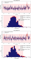 |
Fig. A.1 Light curves of TM5 and TM7 (without on-chip filter) filtered from events outside 3σ interval (shaded red area). |
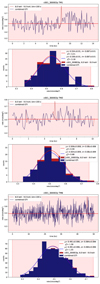 |
Fig. A.2 Light curves of TM1, TM2, and TM6 (with on-chip Alter) filtered from events outside 3σ interval (shaded red area). |
References
- Abell, G. O., Corwin, Harold G.J., & Olowin, R.P. 1989, ApJS, 70, 1 [NASA ADS] [CrossRef] [Google Scholar]
- Ade, P. A. R., Aghanim, N., Arnaud, M., et al. 2013, A&A, 550, A134 [NASA ADS] [CrossRef] [EDP Sciences] [Google Scholar]
- Arnaud, K. A. 1996, ASP Conf. Ser., 101, 17 [Google Scholar]
- Asplund, M., Grevesse, N., Sauval, A. J., & Scott, P. 2009, ARA&A, 47, 481 [NASA ADS] [CrossRef] [Google Scholar]
- Biffi, V., Dolag, K., Reiprich, T. H., et al. 2022, A&A, 661, A17 (eROSITA EDR SI) [Google Scholar]
- Boller, T., Liu, T., Weber, P., et al. 2021, A&A, 647, A6 [EDP Sciences] [Google Scholar]
- Botteon, A., van Weeren, R. J., Brunetti, G., et al. 2020, MNRAS, 499, L11 [Google Scholar]
- Böhringer, M., Reiprich, T. H., Bulbul, E., et al. 2021, A&A, 647, A3 [NASA ADS] [CrossRef] [EDP Sciences] [Google Scholar]
- Brunner, H., Liu, T., Lamer, G., et al. 2022, A&A, 661, A1 (eROSITA EDR SI) [NASA ADS] [CrossRef] [EDP Sciences] [Google Scholar]
- Böhringer, H., Schuecker, P., Guzzo, L., et al. 2001, A&A, 369, 826 [Google Scholar]
- Campusano, L. E., Kneib, J.-P., & Hardy, E. 1998, ApJ, 496, L79 [NASA ADS] [CrossRef] [Google Scholar]
- Chow-Martinez, M., Andernach, H., Caretta, C. A., & Trejo-Alonso, J. J. 2014, MNRAS, 445, 4073 [CrossRef] [Google Scholar]
- Churazov, E., Khabibullin, I., Lyskova, N., Sunyaev, R., & Bykov, A. M. 2021, A&A, 651, A41 [NASA ADS] [CrossRef] [EDP Sciences] [Google Scholar]
- Cypriano, E. S., Sodré, L.Jr., Campusano, L.E., et al. 2001, AJ, 121, 10 [NASA ADS] [CrossRef] [Google Scholar]
- De Luca, A., & Molendi, S. 2004, A&A, 419, 837 [NASA ADS] [CrossRef] [EDP Sciences] [Google Scholar]
- Foster, A. R., Ji, L., Smith, R. K., & Brickhouse, N. S. 2012, ApJ, 756, 128 [Google Scholar]
- Freyberg, M., Perinati, E., Pacaud, F., et al. 2020, SPIE, 11444, 195 [Google Scholar]
- Fujita, Y., Tawa, N., Hayashida, K., et al. 2008, PASJ, 60, S343 [Google Scholar]
- Galli, M., Cappi, A., Focardi, P., Gregorini, L., & Vettolani, G. 1993, A&AS, 101, 259 [NASA ADS] [Google Scholar]
- Ghirardini, V., Bulbul, E., Hoang, D. N., et al. 2021, A&A, 647, A4 [EDP Sciences] [Google Scholar]
- Gilli, R., Comastri, A., & Hasinger, G. 2006, A&A, 463, 79 [Google Scholar]
- Govoni, F., Orrù, E., Bonafede, A., et al. 2019, Science, 364, 981 [Google Scholar]
- Huchra, J. P., Macri, L. M., Masters, K. L., et al. 2012, ApJS, 199, 26 [Google Scholar]
- Hudson, D. S., Mittal, R., Reiprich, T. H., et al. 2010, A&A, 513, A37 [NASA ADS] [CrossRef] [EDP Sciences] [Google Scholar]
- Katayama, H., Hayashida, K., & Hashimotodani, K. 2001, PASJ, 53, 1133 [Google Scholar]
- Kuntz, K. D., & Snowden, S. L. 2008, A&A, 478, 575 [NASA ADS] [CrossRef] [EDP Sciences] [Google Scholar]
- Lovisari, L., Reiprich, T. H., & Schellenberger, G. 2015, A&A, 573, A118 [NASA ADS] [CrossRef] [EDP Sciences] [Google Scholar]
- Lumb, D. H., Warwick, R. S., Page, M., & De Luca, A. 2002, A&A, 389, 93 [CrossRef] [EDP Sciences] [Google Scholar]
- Markevitch, M., & Vikhlinin, A. 2007, Phys. Rep., 443, 1 [Google Scholar]
- McCammon, D., Almy, R., Apodaca, E., et al. 2002, ApJ, 576, 188 [NASA ADS] [CrossRef] [Google Scholar]
- Merloni, A., Predehl, P., Becker, W., et al. 2012, eROSITA Science Book: Mapping the Structure of the Energetic Universe [Google Scholar]
- Mirakhor, M. S., Walker, S. A., & Runge, J. 2022, MNRAS, 509, 1109 [Google Scholar]
- Nandra, K., Barret, D., Barcons, X., et al. 2013, ArXiv eprints [arXiv:1386.2307] [Google Scholar]
- Nascimento, R. S., Ribeiro, A. L. B., Trevisan, M., et al. 2016, MNRAS, 460, 2193 [NASA ADS] [CrossRef] [Google Scholar]
- Predehl, P., Andritschke, R., Arefiev, V., et al. 2021, A&A, 647, A1 [EDP Sciences] [Google Scholar]
- Raymond, J. C., & Smith, B. W. 1977, ApJS, 35, 419 [NASA ADS] [CrossRef] [Google Scholar]
- Reiprich, T. H. 2017, Astron. Nach., 338, 349 [NASA ADS] [CrossRef] [Google Scholar]
- Reiprich, T. H., & Böhringer, H. 2002, ApJ, 567, 716 [Google Scholar]
- Reiprich, T. H., Sarazin, C. L., Kempner, J. C., & Tittley, E. 2004, ApJ, 608, 179 [Google Scholar]
- Reiprich, T. H., Basu, K., Ettori, S., et al. 2013, Space Sci. Rev., 177, 195 [Google Scholar]
- Reiprich, T. H., Veronica, A., Pacaud, F., et al. 2021, A&A, 647, A2 [EDP Sciences] [Google Scholar]
- Sanders, J. S. 2006, MNRAS, 371, 829 [Google Scholar]
- Sanders, J. S., Biffi, V., Bröggen, M., et al. 2022, A&A, 661, A36 (eROSITA EDR SI) [NASA ADS] [CrossRef] [EDP Sciences] [Google Scholar]
- Schellenberger, G., & Reiprich, T. H. 2017, MNRAS, 469, 3738 [CrossRef] [Google Scholar]
- Struble, M. F., & Rood, H. J. 1999, ApJS, 125, 35 [Google Scholar]
- Sunyaev, R., Arefiev, V., Babyshkin, V., et al. 2021, A&A, 656, A132 [NASA ADS] [CrossRef] [EDP Sciences] [Google Scholar]
- Tanaka, Y., Inoue, H., & Holt, S. S. 1994, PASJ, 46, L37 [NASA ADS] [Google Scholar]
- Veronica, A., Su, Y., Biffi, V., et al. 2022, A&A, 661, A46 (eROSITA EDR SI) [NASA ADS] [CrossRef] [EDP Sciences] [Google Scholar]
- Whelan, B., Reiprich, T. H., Pacaud, F., et al. 2021, A&A, submitted [arXiv:2106.14545] [Google Scholar]
- Willingale, R., Starling, R. L. C., Beardmore, A. P., Tanvir, N. R., & O’Brien, P.T. 2013, MNRAS, 431, 394 [NASA ADS] [CrossRef] [Google Scholar]
- Wilms, J., Allen, A., & McCray, R. 2000, ApJ, 542, 914 [Google Scholar]
- Xu, W., Ramos-Ceja, M. E., Pacaud, F., Reiprich, T. H., & Erben, T. 2018, A&A, 619, A162 [NASA ADS] [CrossRef] [EDP Sciences] [Google Scholar]
XMM-Newton SAS documentation, asmooth description: https://xmm-tools.cosmos.esa.int/external/sas/current/doc/asmooth/index.html
All Tables
PV observation (ObsID: 300003, SRG Observing mode: pointing) of the AGN 1H 0707–495 and the A3408 galaxy cluster on 11 October 2019 by eROSITA.
Estimated cluster properties of A3408 applying the M500 - T relation from Lovisari et al. (2015).
Temperature values of the outer bins within 4–12 in the east (TE) and west (TW) of the temperature map.
All Figures
|
Fig. 1 Particle background-subtracted and exposure-corrected photon image of A3408 with TM 1, 2, 5, 6, and 7 in the soft band (0.3–2.3 keV energy band for TM 1, 2, and 6 and 1.0–2.3 keV energy band for TM 5 and 7) in logarithmic scale. |
| In the text | |
|
Fig. 2 Adaptively smoothed particle background-subtracted and exposure-corrected photon image in the soft band (0.3–2.3 keV energy band for TM 1, 2, and 6 and 1.0–2.3 keV energy band for TM 5 and 7) in logarithmic scale. There seems to be diffuse emission out to beyond r200 (dashed white line) in the western direction, including possibly infalling galaxy groups (“extended source”) in the east at a similar redshift as A3408 and south (no redshift estimate available). |
| In the text | |
|
Fig. 3 Particle background-subtracted and exposure-corrected photon image of TM 1, 2, 5, 6, and 7 in the soft band in logarithmic scale. Left: four sectors, SW, SE, NW, and NE out to r200 (dashed white lines), are illustrated. These areas were used to extract the counts for the surface brightness profiles. Center: elliptical annuli (white) out to a semimajor axis of 19 and a semiminor axis of 9.5. The annuli have the same eccentricity and angle of 40 deg, which were chosen to be visually aligned to the cluster shape. These areas were used to obtain temperature, metallicity, and normalization profiles. Furthermore, the temperature map was determined within a circular area of 19 (magenta) to ensure enough counts in the source regions for spectral fitting. Right: calculated characteristic radii r500 (green), r200 (dashed white) and r100 (yellow) of A3408 and A3407 from analyzing ROSAT data and applying the relations r100 ≈ 1.36r200 and r500 ≈ 0.65r200 in Reiprich et al. (2013). |
| In the text | |
|
Fig. 4 Surface brightness profiles obtained in four different sectors (SW, SE, NW, and NE; as illustrated in Fig. 3, left). The CXB level is shown as the dashed orange line, and r500 and r200 are shown as dashed gray and black lines, respectively. |
| In the text | |
|
Fig. 5 eROSITA spectrum of TM 6 in 0.2r500 to 0.5r500 with corresponding model. |
| In the text | |
|
Fig. 6 Normalization (top), temperature (middle), and metallicity (bottom) profiles of A3408 using elliptical annuli, where r represents the semimajor axis. The dashed gray lines indicate r500 of the cluster. |
| In the text | |
|
Fig. 7 Temperature map of A3408. The eROSITA FoV (blue) and r200 (dashed white line) are indicated. Left: temperature map with an additional annulus of 4–12 (black) for visualization. Center, temperature map with surface brightness contours generated from the particle background-subtracted and exposure-corrected soft-band image overlaid in black. Right: relative errors for each temperature in the corresponding bin. |
| In the text | |
|
Fig. 8 Comparison of surface brightness profiles obtained in two sectors (SE and NW, as illustrated in the left panel of Fig. 3). The CXB level is shown as a dashed orange line, and r500 and r200 are shown as dashed gray and black lines, respectively. |
| In the text | |
|
Fig. A.1 Light curves of TM5 and TM7 (without on-chip filter) filtered from events outside 3σ interval (shaded red area). |
| In the text | |
|
Fig. A.2 Light curves of TM1, TM2, and TM6 (with on-chip Alter) filtered from events outside 3σ interval (shaded red area). |
| In the text | |
Current usage metrics show cumulative count of Article Views (full-text article views including HTML views, PDF and ePub downloads, according to the available data) and Abstracts Views on Vision4Press platform.
Data correspond to usage on the plateform after 2015. The current usage metrics is available 48-96 hours after online publication and is updated daily on week days.
Initial download of the metrics may take a while.