| Issue |
A&A
Volume 661, May 2022
The Early Data Release of eROSITA and Mikhail Pavlinsky ART-XC on the SRG mission
|
|
|---|---|---|
| Article Number | A41 | |
| Number of page(s) | 21 | |
| Section | Stellar structure and evolution | |
| DOI | https://doi.org/10.1051/0004-6361/202141105 | |
| Published online | 18 May 2022 | |
Phase-resolved X-ray spectroscopy of PSR B0656+14 with SRG/eROSITA and XMM-Newton★
1
Leibniz-Institut für Astrophysik Potsdam (AIP),
An der Sternwarte 16,
14482
Potsdam,
Germany
e-mail: This email address is being protected from spambots. You need JavaScript enabled to view it.
2
Purple Mountain Observatory, Key Laboratory of Dark Matter and Space Astronomy, Chinese Academy of Sciences,
Nanjing
210008,
PR China
3
Potsdam University, Institute for Physics and Astronomy,
Karl-Liebknecht-Straße 24/25,
14476
Potsdam,
Germany
4
Institut für Astronomie und Astrophysik,
Sand 1,
72076
Tübingen,
Germany
5
Astronomy Department, Kazan (Volga region) Federal University,
Kremlyovskaya str. 18,
420008
Kazan,
Russia
6
Space Research Institute of the Russian Academy of Sciences,
Profsoyuznaya str. 84/32,
117997
Moscow,
Russia
7
Max-Planck-Institut für extraterrestrische Physik,
Gießenbachstraße 1,
85748
Garching,
Germany
8
Ioffe Institute,
Politekhnicheskaya 26,
194021
Saint Petersburg,
Russia
Received:
16
April
2021
Accepted:
30
June
2021
Abstract
We present a detailed spectroscopic and timing analysis of X-ray observations of the bright pulsar PSR B0656+14. The observations were obtained simultaneously with eROSITA and XMM-Newton during the calibration and performance verification phase of the Spektrum-Roentgen-Gamma mission (SRG). The analysis of the 100 ks deep observation of eROSITA is supported by archival observations of the source, including XMM-Newton, NuSTAR, and NICER. Using XMM-Newton and NICER, we first established an X-ray ephemeris for the time interval 2015 to 2020, which connects all X-ray observations in this period without cycle count alias and phase shifts. The mean eROSITA spectrum clearly reveals an absorption feature originating from the star at 570 eV with a Gaussian σ of about 70 eV that was tentatively identified in a previous long XMM-Newton observation. A second previously discussed absorption feature occurs at 260–265 eV and is described here as an absorption edge. It could be of atmospheric or of instrumental origin. These absorption features are superposed on various emission components that are phenomenologically described here as the sum of hot (120 eV) and cold (65 eV) blackbody components, both of photospheric origin, and a power law with photon index Γ = 2 from the magnetosphere. We created energy-dependent light curves and phase-resolved spectra with a high signal-to-noise ratio. The phase-resolved spectroscopy reveals that the Gaussian absorption line at 570 eV is clearly present throughout ~60% of the spin cycle, but it is otherwise undetected. Likewise, its parameters were found to be dependent on phase. The visibility of the line strength coincides in phase with the maximum flux of the hot blackbody. If the line originates from the stellar surface, it nevertheless likely originates from a different location than the hot polar cap. We also present three families of model atmospheres: a magnetized atmosphere, a condensed surface, and a mixed model. They were applied to the mean observed spectrum, whose continuum fit the observed data well. The atmosphere model, however, predicts distances that are too short. For the mixed model, the Gaussian absorption may be interpreted as proton cyclotron absorption in a field as high as 1014 G, which is significantly higher than the field derived from the moderate observed spin-down.
Key words: stars: neutron / X-rays: stars / pulsars: individual: PSR B0656+14
Based on observations obtained with XMM-Newton, an ESA science mission with instruments and contributions directly funded by ESA Member States and NASA.
© ESO 2022
1 Introduction
PSR B0656+14 (hereafter B0656) is an intermediate-aged pulsar that was observed at all wavelengths from the radio regime up to gamma energies. It is the brightest of the “Three Musketeers”, which were nicknamed by Becker & Trümper (1997) because of their exceptional brightness and similar periods, ages, and spectral energy distribution (SED). Pulsar B0656 was one of the 27 rotation-powered pulsars that were previously detected with ROSAT (Becker & Trümper 1997). It shows thermal and nonthermal radiation components.
Initially, the thermal component was modeled as a black-body, but already Possenti et al. (1996) found the ROSAT spectrum to be more complex. The combined ROSAT/ASCA X-ray spectrum then revealed a phenomenological model that is valid with modifications until today. It consists of two blackbody components from the stellar surface and a power-law tail of magnetospheric origin (Greiveldinger et al. 1996). This model was confirmed by CCD and grating spectroscopic observations performed with Chandra by Pavlov et al. (2002). Using the Chandra grating (LETG) spectrum, Marshall & Schulz (2002) stressed that no absorption line was found in the spectral range 0.2–1.0 keV. Their phase-average spectrum was well represented with the sum of two blackbodies. First XMM-Newton observations in timing and imaging (small window) mode were presented by De Luca et al. (2005). They confirmed the earlier spectral model. The much improved photon counting statistics for the first time allowed tracing the various spectral components through the spin cycle of the Prot ≃ 385 ms pulsar with the two blackbody components varying in antiphase. Recently, Arumugasamy et al. (2018) reported a possible phase-dependent absorption feature with a central energy between 0.5–0.6 keV in coordinated XMM-Newton/NuSTAR observations. The inclusion of a Gaussian absorption line for about 50% of the spin cycle improved the phenomenological model.
Harding et al. (2019) reported a summary of NICER observations showing three distinct hot spots that cover different energy bands and rotational phases: a cool thermal radiation component from the entire neutron star surface, a smaller hot spot presumably from polar cap heating, and an additional component at intermediate temperature. The X-ray emission peaks from these hot spots occur at different rotation phases that are also different from the phases of the radio and gamma-ray peaks. The complex variation in temperature throughout the surface possibly suggests evolution of multipolar magnetic field structure.
The most recent account of the phase-averaged X-ray spectrum of B0656 was given by Zharikov et al. (2021), who on the one hand confirmed the earlier spectral model by Arumugasamy et al. (2018), but also refined it by including infrared, optical, and ultraviolet data (IR, opt, and UV). The spectral energy distribution established in this paper is best described by a broken power law from the magnetosphere plus the double blackbody with superposed absorption line at ~0.5 keV originating from the stellar surface. The inclusion of the low-energy data indicates a smaller NS radius than is obtained from the X-ray spectral fits alone, which otherwise overpredict the observed IR, opt, and UV emission from the object.
The possible existence of an absorption line in the soft part of the spectrum triggered the Spektrum-Roentgen-Gamma (SRG)/eROSITA observation of B0656 in its calibration and performance verification phase for 100 ks. At this early phase in the SRG mission, calibration uncertainties were to be expected. We therefore asked the XMM-Newton project scientist to support the SRG mission and this observation in particular with a simultaneous observation of our target on director’s discretionary time. Thankfully, this time was granted, and the two observatories obtained data simultaneously.
These recent XMM-Newton data have been presented by Zharikov et al. (2021) in their analysis of the mean spectrum of the source. They are placed in context with eROSITA in the current paper, where a spin-phase resolved analysis is presented. Here we focus on the spectral analysis of the coordinated eROSITA/XMM-Newton-observations, but take other X-ray data into account to describe the overall spectral energy distribution (including NuSTAR) and to improve the timing solution (NICER) of the pulsar. We also briefly address calibration items as far as the timing system is concerned.
The targeted observations of B0656, some 8 deg above the galactic plane, at the same time provide one of the deepest looks into the Galaxy by eROSITA in the years to come. Given the 63’ field of view, such a deep observation is a fully fledged X-ray survey in its own right. More than 960 X-ray sources were found serendipitously in the same observation (0.6–2.3 keV; all telescope modules). The comprehensive source catalog from this observation will be published in a separate paper (Lamer et al., in prep.).
The paper is structured as follows. In Sect. 2, we describe the observational data set we analyzed and the data reduction. The results are detailed in Sect. 3. In Sect. 3.1, we present a new timing solution for the pulsar and analysis of the light curves. A spectral analysis of the phase-averaged and the phase-resolved spectra using models of the phenomenological and more physically motivated neutron star atmosphere and the condensed surface is presented in Sect. 3.2. Our main results are summarized and discussed in Sect. 4. We provide additional timing and spectral information about the eROSITA data in the appendix. When computing dimensions of emitting areas and luminosity, we use the distance to B0656 from the VLA radio parallax of  pc (Brisken et al. 2003).
Joint and supporting SRG/eROSITA, XMM-Newton, and NuSTAR observations of PSR B0656+14.
2 Observations and reductions
2.1 SRG/eROSITA
The observations of PSR B0656+14 with SRG/eROSITA were the first PV-phase observations to be conducted with all seven telescope modules (TM) of the German eROSITA collaboration eROSITA_DE after an extended commissioning and calibration phase of the instrument and the observatory as a whole. They were performed on October 14, 2019, for a nominal exposure of 100 ks (see Table 1). Two anomalies occurred: TM1 did not reveal science-grade data, and a time shift of the central spacecraft clock of −0.345 s was applied during the observations of our target at the onboard execution time of 2019-10-14 23:00:45 (UT; cf. Appendices A and B for more information).
All eROSITA cameras were operated in FrameStore mode with the PMWORK and FILTER setup. The data were reduced and analyzed with the eSASS software system eSASSusers_2010091 within the 0.2–10 keV energy band. TMs 1, 2, 3, 4, and 6 are operated with an aluminium filter directly deposited on the CCD, while TM5 and TM7 are operated with a filter that consists of a polyimide foil with an aluminium layer. The thickness of the aluminium layer is lower, which gives TM5 and TM7 higher sensitivity, in particular, at soft X-ray energies. Interestingly, these two also show time-variable light leaks which (may) impact their usability for soft X-ray studies (see Predehl et al. 2021, for further details).
In the following, the summed signal from the cameras with on-chip filter is referred to as (virtual) telescope module TM8 (here without TM1), the summed signal from the cameras without the filters is referred to as TM9, and the sum of all physical TMs as TM0 (again, in this paper without TM1). At the time of writing, the energy calibration of TM9 is less reliable than that of TM8, regardless of whether a particular observation is affected by light leaks. The final spectral results presented below are therefore derived for TM8 in the main body of the paper. For cross-calibration purposes, the results of individual TMs and TM0 and TM9 are reported in Appendix D. Our timing analysis is based on all active detectors.
The event files were filtered for periods of high background activity with the eSASS task flaregti. The flaring count rate level (threshold) of each detector for the duration of the observation was determined on the basis of the mean surface brightness of local pixels in a predefined spatial grid. We adopted the 2.2–10 keV energy band to minimize contamination from the central source and a time bin size of 100 s; bright sources in the field of view were masked by default. The analysis shows typical threshold values per detector around 2 s−1 deg−2, which were then adopted for GTI filtering. Averaged over all telescope modules, the percentage of time loss due to flares is low, about 1.6%. We inspected the GTI-filtered images that are created for all TMs in different energy ranges for artefacts and possible light leaks. We found that only TM7 shows a pronounced light leak visible at soft energies, while TM5 is apparently unaffected. A color composite of the GTI-filtered eROSITA image is shown in Fig. 1.
We performed source detection based on maximum likelihood (ML) PSF fitting to generate catalogs in various energy bands (see, e.g., Brunner et al. 2022; Liu et al. 2022, for details). For maximum sensitivity, all GTI-filtered event tables of the six telescope modules and all valid photon patterns were considered. In Table 2 we list the number of sources detected in the field of view in three broad energy bands (soft, 0.2–0.6 keV, medium, 0.6–2.3 keV, and hard, 2.3–5 keV) and the source characterization parameters from ML PSF fitting.
The catalogs were then used to optimize the coordinates and sizes of the source and background extraction regions with the “auto” option of the srctool task. In this mode, the task can also be used to identify neighboring sources (“contaminants”) whose PSF overlaps the regions of interest. We chose the source (circular) and background (annular) regions to be centered around the target coordinates as determined with ermldet in the soft energy band. Additionally, we screened the catalogs for spurious extended detections, which are erroneously identified as contaminants in the wings of the target PSF2. The various energy bands were used to assess the likelihood of the X-ray sources detected within 2.5′ away from the aimpoint.
According to this analysis, we adopted an extraction radius of 150″ for the target and determined “exclusion zones” around the position of seven contaminants detected in the medium and hard energy bands (Fig. 2; left). The seven sources have a detection likelihood within 12–400 and counts within 60–3500 (0.6–2.3 keV). Because the pulsar is bright below 2.3 keV, the blind application of the srctool functionality leads to a background annulus with inner and outer radii of ~4–5.5′ and ~27–35′, respectively. To further minimize (below 2%) the contamination from the central source and avoid uncertainties due to vignetting effects at the very edge of the eROSITA field of view, we decided instead to adopt a narrower 5′ wide background annulus with an inner radius of 10′. All 152 contaminants detected in the 0.6–2.3 keV energy band were then excluded from this region (Fig. 2; right).
In Fig. 3, we show the distribution of photon patterns (i.e., the relative fraction of singles, doubles, triples, and quadruples) as a function of energy for the events detected at aimpoint. Only the detectors with on-chip filter were considered. Solid curves show the expected distribution according to the model in the calibration database. The overall trend of the pattern distribution follows the calibrated trend and is also consistent with that of other X-ray bright and nearby isolated neutron stars observed during the CalPV phase (Pires et al., in prep.). On the other hand, the lack of singles and excess of doubles and triples with respect to the calibrated pattern distribution is remarkable within 0.2–2 keV. This mismatch is understood to be due to several factors that include the exact subpixel location of the photons in the detector, contamination from detector noise below 0.4 keV, and the low-energy threshold applied to the data for telemetry reasons (especially important for the detectors affected by the optical leak).
We extracted light curves to measure the mean count rate of the pulsar in the 0.2–0.6 keV, 0.6–5 keV, and 0.2–5 keV energy bands, using a time bin size of 100 s. To this end, we used the flare-filtered event lists and corrected the number of photons in each time bin for the difference in source and background area size before subtracting the background, while also multiplying them with a PSFcorrection factor computed from the eROSITA 2dpsf files. The resulting mean count rates are shown in Table 3. Detectors 5 and 7, which are more sensitive at soft X-rays, show a higher count rate at these energies than TM2, 3, 4, and 6. All exposures are consistent with a constant flux.
The times of arrival of the photons were converted from the local satellite into the Solar System barycentric frame using the HEASOFT task barycen, the JPL-DE405 ephemeris table, the target coordinates from Arumugasamy et al. (2018), and a suitable orbit file covering the epoch of the observation. For the latter, we converted the file with information on the spacecraft position and velocity as provided by NPOL into the FITS format required by barycen. Likewise, some header keywords in the eROSITA event files were edited to comply with the tool3. The correction was performed separately for each detector to take the time stamps and GTIn extensions of each instrument individually into account and correct for it. The corrected event files were then merged back into a master table with separate GTIn extensions per detector, as is standard in an eSASS analysis.
The cleaned and barycenter-corrected event lists were used to extract the scientific products, spectra and phase-folded light curves, that were further adopted in the analysis (Sect. 3). To generate phase-resolved spectra, we split the source photons according to the spin phase of the pulsar into multiple event files (see Sect. 3.1.2 for details). We kept the original extensions of the pipeline-processed event table to ensure compatibility with eSASS. The GTIn extensions were updated accordingly to cover the respective phases of interest. Finally, the eSASS task srctool was applied to generate the individual spectrum of each phase interval.
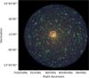 |
Fig. 1 Composite eROSITA image produced from selected photons in three different energy bands (red: 0.2–0.5 keV, green: 0.5–1.5 keV, and blue: 1.5–7 keV) showing the large eROSITA field of view. The pulsar B0656 is centrally located at the aimpoint. The white rectangle shows the field of view of the XMM-Newton observations that were simultaneously conducted with EPIC-pn in the small-window mode. |
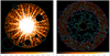 |
Fig. 2 Extraction regions we adopted in the analysis. The source and background regions are centered at right ascension 104.951117 deg and declination +14.239175 deg. The exclusion zones of contaminants are shown as cyan circles with a red bar. Left. source extraction radius (yellow) of 150″ (TM2; 0.2–10 keV). Right. background annulus (magenta) has inner and outer radii 10′ and 15′, respectively (TM6; 0.2–10 keV). |
Results of source detection and ML PSF fitting.
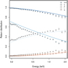 |
Fig. 3 Distribution of photon pattern fractions as a function of energy. The observed fractions of singles (s), doubles (d), singles and doubles (s + d), triples (t), and quadruples (q) are shown as data points for the TM8 detector combination. Solid lines show the expected (theoretical) pattern distribution in the 0.2–2 keV energy band. |
Mean count rates of PSR B0656+14 per eROSITA detector.
2.2 XMM-Newton
XMM-Newton observed PSR B0656+14 on three occasions in 2001, 2015, and in 2019. The observation in 2019 was made simultaneously with eROSITA (Sect. 1; see also De Luca et al. 2005; Arumugasamy et al. 2018; Zharikov et al. 2021). For the 2019 observation, we chose to observe the pulsar with the same instrumental setup as in 2015, that is, the EPIC-pn and MOS instruments in small-window (SW) and timing (TI) mode, respectively. All EPIC exposures were performed with the THIN1 filter. The RGS1 and RGS2 instruments were used in SES spectroscopy mode. We do not discuss the OM exposures in our analysis.
We reduced the observations with the XMM-Newton Science Analysis (SAS) software, version 18.0.0, following standard procedure and applying current calibration files. We extracted event lists for the EPIC instruments using the meta-tasks emproc and epproc. The time stamps of the photons, GTI extensions, and time-related header keywords were barycentered with the SAS task barycen. In neither the 2015 nor 2019 observations did MOS1 deliver science-grade data. We do not include MOS2 in the analysis because its quality is lower than pn, as verified by preliminary analysis.
We adopted a circular source extraction region of radius 22.5″ for the two pn SW observations. Background events were extracted from two box-like regions on the same CCD as the target, defined so as to avoid out-of-time events along the read-out direction (Fig. 4). We screened the background light curves in the energy range 0.3–12 keV for flares, adopting a bin size of 50 s. Following the prescription of De Luca & Molendi (2004), we defined a rejection threshold of 3σ from the Gaussian mean, based on the observed distribution of count rates. We used the tabgtigen task to generate GTI files and used them to filter the event files with evselect. Only unflagged single and double events (FLAG = 0 PATTERN ≤ 4) were selected. The resulting filtered event list was subsequently adopted for the timing and spectral analysis.
For RGS, we used the EPIC source coordinates as determined with the SAS task emldetect in each observation to generate the instrument spatial masks and energy filters with the SAS routine rgsproc. We identified times of low background activity from the count rate on CCD 9, the closest to the optical axis, and applied a count rate threshold of 0.1 s−1 to filter the GTIs. Because of electronic problems, one CCD chip of each of the RGS detectors failed early in the mission. This affects the spectral coverage between 11 Å and 14 Å and between 20 Å and 24 Å in RGS1 and RGS2, respectively.
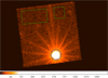 |
Fig. 4 XMM-Newton SW observation of PSR B0656+14, performed simultaneously with eROSITA in October 2019. Source and background extraction regions are overlaid (blue circle with radius 22.5″ and green boxes of sizes 110″ × 58″ (left)and 44″ × 50″ (right); 0.3–12 keV). The image has 63 × 64 pixels, about 4.3 × 4.3′. |
2.3 NuSTAR
To improve hard-band coverage for the spectral analysis, we included the NuSTAR observation of the source listed in Table 1 that was previously reported by Arumugasamy et al. (2018), who obtained the data simultaneously with the 2015 XMM-Newton observation. To reduce the data, we followed the same procedures as described by Zharikov et al. (2021), who used the same observation in their analysis. In particular, the raw data were reprocessed using the nuproducts task from HEASOFTv6.28 and calibration files v20210202. The source spectrum was extracted from a circular region centered on the source with radius of 30″ (independently for each telescope module), while the background was extracted from a nearby source-free region with a radius of 100″, located at approximately the same location as was used by Zharikov et al. (2021). The extracted spectra for both telescope units were grouped to contain at least 25 counts per energy bin and were modeled together with other spectra from other instruments as described in Sect. 3.2.1.
2.4 NICER
To improve the pulsar ephemeris and enable a phase-resolved analysis, we also analyzed NICER observations of the source. We retrieved all NICER observations of the source obtained up to the time of the analysis (March 2021). The NICER master catalog provided by HEASARC lists 93 observations obtained between October 13, 2017, and April 9, 2020, with an exposure time longer than 0. In addition, the 2015 and 2019 XMM-Newton observations were included in the analysis. The 2001 observation was not included because of the large time gap between 2001 and 2015 in which no sufficiently long X-ray observation was obtained. Considering that the shapes of X-ray light curves are energy dependent (see Sect. 3.1.2 and papers by De Luca et al. 2005; Arumugasamy et al. 2018), we only used photons in the range 0.3–2 keV, in which the responses of NICER and XMM-Newton are similar, to avoid possible apparent distortion of the pulse profiles due to differences in the energy response of the two instruments.
All NICER observations listed in Table C.2 were reduced using the current set of calibration files and standard screening criteria4. The arrival times in the resulting event lists were then corrected to the Solar System barycenter and merged in several groups corresponding to observations performed close in time (i.e., separated by gaps of at most two days), as summarized in Table C.2.
3 Analysis and results
3.1 Timing analysis
We used the observation of the pulsar to test the relative timing accuracy of the individual eROSITA TMs. We searched for the pulsar period, using events with energies between 0.3 and 2.0 keV, in the XMM-Newton and individual eROSITA TM exposures applying the  test (Buccheri et al. 1983). Confidence levels on the frequency of the highest
  peak were estimated by maximum likelihood (e.g., Fisher et al. 1990). The results are listed in Table 4 and illustrated in Fig. 5. The Z2 values for TMs 5 and 7 are higher than for the other TMs because the count rates in these modules are much higher. The table also lists the reference periods that are derived by extrapolating recent radio and gamma-ray ephemerides to the date of the joint eROSITA/XMM-Newton campaign (Ray et al. 2011; Johnston & Kerr 2018; Lower et al. 2020)5. Excerpts of the ephemeris parameter files of these three timing solutions are listed in Table C.1.
The periods found from the six eROSITA TMs agree well with each other, but individually and jointly (average period), they deviate from the simultaneous XMM-Newton result and from the radio and γ-ray references. The relative deviation (Pero − Pref)/Pref is (−6.23, −6.14, −6.14, −6.28) × 10−7 from the simultaneous XMM-Newton and the extrapolated periods from the Ray et al. (2011), Johnston & Kerr (2018), and Lower et al. (2020) ephemerides (referred to as JK18 and Low20 in Table 4), respectively.
Part of the deviation between eROSITA and the external references lies in the constantly growing clock drift between the central SRG quartz and the UTC references, which is about 12 ms day−1 (see Appendix B for details). The clock drift accounts for a relative deviation of −1.4 × 10⁻⁷, indicating that the remaining timing calibration uncertainties are to be found in the eROSITA time system.
In the absence of an absolute time reference for eROSITA, we decided to use a local phase convention further in this analysis. Phase zero was defined as the phase of the maximum count rate in a phase-folded X-ray light curve in the energy band 0.3–2.0 keV. To generate phase-folded light curves and phase-binned spectra for both XMM-Newton and eROSITA, we used the mission-specific period and sampled the light curve into 20 phase bins. For eROSITA, we used the weighted average period of the six TMs as given in Table 4, 384.93394(4) ms. To fold the light curves in phase, we defined the phase of X-ray maximum by fitting the sum of the first and second harmonic sine functions,

where φ is the initial arbitrary phase. This model represented the observed data well, as indicated by the reduced  , which took values between 0.78 and 1.41 for 15 degrees of freedom.
The fit revealed a phase of the X-ray maximum that was determined numerically. The offset phase, converted into time, was subtracted from the input photon arrival times to then generate the final phase-folded light curves in the different energy bands. The same procedure was adopted for the EPIC-pn data.
De Luca et al. (2005) established a phase relation between the X-ray maximum and the radio pulse in their analysis of the first XMM-Newton data obtained in 2001. They found that the radio pulse occurred 0.25 ± 0.05 phase units later than the X-ray maximum, where the latter was defined as the maximum bin in the phase-folded X-ray light curve. We were interested whether we would find the same phase relation in the data obtained with XMM-Newton in 2015 and 2019, which both could be placed on an absolute timescale using the JK18 and Low20 ephemerides. However, the slightly longer period determined by Lower et al. (2020) leads to a cycle count difference between the 2015 and 2019 observations of 4.8 spin cycles with respect to the JK18 timing solution. This prevented us from determining the phase offsets between X-ray and radio pulses.
Results of the period search.
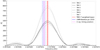 |
Fig. 5 Period search of eROSITA and XMM-Newton data. |

3.1.1 Timing solution of XMM-Newton and NICER
To resolve the issue, we generated our own long-term ephemeris based on X-ray data alone. In particular, NICER and XMM-Newton data reduced as described in Sects. 2.2 and 2.4 were used for this analysis. As already mentioned, all events from both instruments were grouped in several groups separated by gaps not larger than two days, as defined in Table C.2. Folding events in each group separately using the ephemeris by Johnston & Kerr (2018) reveals that the X-ray pulse phase initially appears constant, but then deviations start to grow and eventually reach ~0.35 phase (see Fig. 6). That is, there are significant deviations from this timing solution, although the pulse cycle counting appears to be retained. We therefore base our further analysis on this solution.
It is also interesting to note that the pulse phase of the X-ray peak for the first observation (closest in time to radio data, but still ~614 d after the end of the formal validity period for radio ephemerides) is consistent with the expected phase of the radio peak. This is inconsistent with the findings by De Luca et al. (2005), who found a ~0.25 phase shift between radio and X-rays and suggested that either that radio ephemerides break already for the first observation in our set (i.e., 2015 XMM-Newton observation), or that the offset between radio and X-ray peaks estimated by De Luca et al. (2005) has been estimated incorrectly. To determine the correct cause, a proper solution would be required that includes radio and X-ray data that cover the same observation period. We focused on the X-ray data alone to properly align the NICER and XMM-Newton data.
To improve the estimates of local frequency and frequency derivative values, we first conducted a  search (Buccheri et al. 1983) around the prediction based on Johnston & Kerr (2018) for the period covered by X-ray data, that is, we assumed a zero epoch of MJD 57284 (TDB time system). For this search we concatenated event lists from all observations and maximized the value of the
  statistic calculated using the Stingray (Huppenkothen et al. 2019) software package, starting from the initial values. The updated solution corresponding to the maximum statistic value largely eliminates the observed phase drift of the X-ray pulses and allows obtaining a high-quality template pulse profile by averaging all observations. This in turn allows determining accurate pulse times of arrival (TOAs) for individual data groups and estimating a final ephemeris using the proper phase-connection. To do this, events in each group were folded separately using the start time of a given interval as a folding epoch and the local frequency and frequency derivative estimates obtained above. The average template pulse profile was then directly fit to the resulting profiles to determine the phase shifts between them (we also allowed for scaling in intensity of the template). The phase shift was then converted into a time shift using the initial estimate of the local pulse frequency and was added to folding epoch to determine TOAs for each group listed in Table C.2.
The observed TOAs were then modeled assuming a constant spin-down rate, that is, using the Taylor expansion in phase ϕ of the form

where t0 = MJD 57284 is our reference epoch, and v0,  are the spin frequency and frequency derivative at that time. Considering the potential presence of timing noise that effectively increases the uncertainty of individual TOA estimates, we used the nested sampling Monte Carlo algorithm MLFriends (Buchner 2014, 2017) implemented in the UltraNest6 package for the final fit to derive posterior probability distributions and the Bayesian evidence for individual parameters. The best-fit residuals with regard to our final solution are presented in Fig. 6. They correspond to v0=2.5978943932(l) Hz and
  = 3.70791(2) × 10−13 Hz s−1, where parameter values and uncertainties are derived from their final posterior probability distributions. We emphasize that the solution above is an approximation that is valid for the period from MJD 57284 to MJD 58866, and a joint fit of X-ray and radio arrival times over a longer baseline is required to determine a final timing solution for the pulsar.
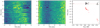 |
Fig. 6 Phaseograms showing pulse proflies in 0.3–2 keV for individual data groups listed in Table C.2 folded using Johnston & Kerr (2018) (left) and the updated ephemeris (middle) obtained in this work. The phase residuals to the best-fit solution (black symbols with error bars) and for the Johnston & Kerr (2018) solution (red, zerophase corresponds to the phase of the radio peak, and errors are omitted for clarity) are also shown in the right panel. |
3.1.2 Phase-folded light curves
Using the timing solution from Sect. 3.1.1, we created phase-folded pulse profiles in various energy bands and binned them into 20 phase bins (Fig. 7). Phase zero was defined as the time of the X-ray maximum in the energy band 0.3–2.0 keV, which was determined by the harmonic fit described above. As noted previously (De Luca et al. 2005; Arumugasamy et al. 2018), the phase of the X-ray maximum is energy dependent. The energy bands of the light curves in Fig. 7 were chosen to highlight the variability of the main spectral components: the cool blackbody, the region in which the absorption feature occurred, the hot blackbody, and the power-law tail. Our analysis reveals that the shapes of the light curves in the various bands and their phase relation were found to be the same in 2001, 2015, and in 2019. In Table 5 we list the phase of the X-ray maximum and the pulsed fraction per energy band per mission for the 2019 eROSITA/XMM-Newton campaign. The pulsed fractions were calculated from the maximum and minimum count rates in the phase-folded light curves using

while the error was propagated from the errors of the maximum and minimum count rates.
The low-energy band (1) shows a slow increase and a fast decrease toward a minimum at phase 0.35. At all occasions, it shows a shoulder at phase 0.6, which is the same phase as that of the minimum of the intermediate band (3), which traces the hotter blackbody. At this energy (band 3), the light curve is almost symmetric, as expected from simple foreshortening and projection of a well-behaved, that is, symmetric heated spot on the NS surface. The phase offset between the soft band (1) and the intermediate band (3) is significant. The hot blackbody peaks at phase 0.06, that is, 0.1 phase units later than the cold blackbody (see also Sect. 3.2.2 below for the results of phase-resolved spectroscopy). The intermediate band (2) behaves very differently from the blackbody-dominated bands (1) and (3). It peaks at about phase 0.65, that is, at the shoulder of band (1), and has a much shallower variability amplitude. Although this band was chosen to trace the absorption feature, the observed light curve shape, which differs strongly from bands (1) and (3), is not due to the absorption feature. This weak feature has a much smaller impact on the shape of the light curves compared to the continuum emission processes. The presence of the shoulder in band (1), which coincides with the maximum in band (2), indicates a more complex emission region than that of a symmetric cold spot (colder than the hot blackbody component). Either emission is from one structured cold region or from a third region with a temperature that is not much different from the region that causes the main maximum in band (1).
The hard band is photon starving, and the derived parameters have large uncertainties. Its low energy boundary was chosen such that the contribution of the hot blackbody was below 3%. At the S/N and the phase resolution achieved with our observations, it may be described with just a more or less symmetrical bright phase and a main minimum that occurs at phase 0.40–0.45. The maximum occurs at about phase 0.9–1.0.
It is worth noting that phase-smearing of eROSITA data cannot be recognized. The frame time of the eROSITA cameras is 50 ms, which corresponds to <8 independent phase bins per spin revolution. The EPIC-pn small window mode has a frame time of 5.7 ms (67 independent phase bins). As shown in Fig. 7 and Table 5, the pulsed fractions of the light curves in band (1) are the same for eROSITA and XMM-Newton, while only little degradation of the pulsed fraction is seen in eROSITA in bands (2) and (3) despite the lower sampling.
In previous studies involving data from XMM-Newton, energy-resolved light curves were generated as well (De Luca et al. 2005; Arumugasamy et al. 2018, their figures 6 and 9, respectively). Slightly different energy passbands and ten phase bins were used for all light curves. All curves in the soft band, dominated by the cool blackbody, are very similar, with a shoulder on the rising branch. Our curve for band 3, dominated by the hot blackbody, is slightly dissimilar compared to the others. Ours appears rather symmetric, with a small shoulder on the descending branch that appears more pronounced in the other works. The pulsed fraction is highest in all studies in band 4, which is dominated by the power law. The curve shown by Arumugasamy et al. (2018) still appears to be different from ours. It has one bin at their phase 0.45, with a rate as high as during the main hard pulse, that is, at phase ~0.1, which we did not find in the two data sets from XMM-Newton or in the eROSITA data.
A complementary view on the energy- and phase-dependent variability is given in Fig. 8, which shows the photons in the soft energy range (0.3–1.5 keV) arranged as a trailed spectrogram with the mean subtracted. It shows that the light-curve maxima below 0.45 keV and above 0.7 keV are stable in phase. It also shows a transition region between 0.45 and 0.7 keV with a strongly variable phase of maximum emission. Above an energy of ~0.7 keV, the maximum phase is apparently stable. Our figure can be compared with the corresponding Fig. 10 from Arumugasamy et al. (2018), which shows the same features, but for a smaller energy range.
Pulsed fractions (pf) and phases of pulse maxima (φmax) in different energy bands for the 2019 eROSITA/XMM-Newton campaign.
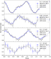 |
Fig. 7 Background-subtracted eROSITA and XMM-Newton pulse profile in different energy bands. The original data were averaged into 20 phase bins at soft and medium energies and averaged into 10 phase bins at hard energies. The light curves are shifted to a common phase, where phase zero is defined as the maximum of the main pulse (see the text for details). |
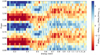 |
Fig. 8 Trailed spectrogram of the eROSITA pulse profile, with phase and energy along the y– and x–axes, respectively. The mean spectrum was subtracted from the original data. Color thus indicates a positive or negative deviation from the mean. Excess values were normalized to their errors. The pulse profile is shown twice for better visibility. |
3.2 Spectral analysis
The analysis of the eROSITA data is based on source and background spectra extracted from regions as described in Sect. 2, together with the respective response matrices and ancillary files created for each detector with the eSASS task srctool. We restricted the analysis to GTI-filtered photons with energy within 0.2 keV and 5 keV, beyond which the source signal-to-noise ratio becomes insignificant. The energy channels of each TM spectrum were regrouped with the HEASOFT task grppha to avoid a low (<50) number of counts per spectral bin.
For the EPIC-pn data (Sect. 2.2), we used the SAS tasks rmfgen and arfgen to generate the respective RMF and ARF files for the 2015 and 2019 observations. The spectra were rebinned with the SAS task specgroup to ensure a minimum S/N of 4 while keeping the oversampling of the instrument energy resolution within a factor of 3. The EPIC data were analyzed within 0.3–7 keV, in accordance with the guidelines and calibration status of EPIC-pn in SW mode.
The RGS GTI-filtered event lists were used to extract the source and background spectra in wavelength space using the SAS tasks rgsregions and rgsspectrum, while response matrix files were produced with rmfgen. Only first-order spectra were analyzed. To increase the S/N, we coadded the RGS1 and RGS2 spectra of the 2015 and 2019 observations into two stacked data sets using the SAS task rgscombine; each combined spectrum was then rebinned into 0.165 Å wavelength channels. The defective channels of the RGS cameras (Sect. 2.2) were excluded from the spectral fitting. The coadded background and response files in each detector were taken into account in the spectral fitting as usual. The total data set amounts to 1.935(14) × 104 and 2.496(16) × 104 counts (12–38 Å) in each RGS1/2 camera, respectively, of which about 40% can be ascribed to the background.
To fit the spectra, we used XSPEC 12.10.1f (Arnaud 1996). Unless otherwise noted, the fit parameters were allowed to vary freely within reasonable ranges. Whenever spectra from different instruments were fitted simultaneously, we adopted a renormalization factor between them to take calibration uncertainties into account (see caption of Tables 6 and 7). The photoelectric absorption model and elemental abundances of Wilms et al. (2000) were adopted to account for the interstellar material in the line of sight. Owing to the low absorption toward the target, the choice of abundance table does not significantly affect the results of the spectral fitting.
Results of the phase-averaged spectral modeling.
Results of the phase-resolved spectral modeling.
3.2.1 Phase-averaged X-ray spectrum of PSR B0656+14
The main emission components in the phase-averaged spectrum of PSR B0656+14 are well described in the literature (see, e.g., Zharikov et al. 2021, and references therein). We repeat the exercise here because different time, pattern, and region selection might lead to slightly different source parameters from the missions whose data were available to previous researchers. The inclusion of the data from eROSITA may shed new light on the emission model of PSR B0656+14 and has two aspects. First, we are interested in the level of agreement of spectral parameters between eROSITA and XMM-Newton to assess the calibration uncertainties, and second, given the improved spectral resolution of eROSITA with respect to XMM-Newton, some of the spectral parameters might need to be revised. Moreover, with a fit to the phase-averaged spectrum, we intend to predetermine some of the spectral parameters for the fits to the phase-resolved spectra, which have a lower signal-to-noise ratio per spectral bin.
The basic model we applied to the data consists of the sum of a hot and a cold blackbody, superposed by an absorption feature that is modeled as a Gaussian, plus a power-law hard tail. Everything was modified by interstellar absorption. In XSPEC terminology, this model is written as tbabs((bbodyrad+ bbodyrad+powerlaw)gabs). This was sufficient to describe the NuSTAR and XMM-Newton spectra so far, but the model leaves strong residuals below 0.3 keV in eROSITA data, which indicate the presence of an additional feature of an as yet uncertain nature. If the residuals are not taken into account in the spectral fitting, the corresponding reduced chi-square values are 1.6 and 3 for the simple fit of TM8 and the simultaneous multi-mission fit (245 and 391 degrees of freedom; cf. fit IDs [1] and [2] in Table 6), respectively.
The possible presence of a second absorption line has previously been reported by Zharikov et al. (2021), when the authors included photons below 0.3 keV in their analysis of XMM-Newton data. Here, we tentatively modeled the low-energy residuals as a multiplicative absorption edge7, which is favored over another Gaussian absorption for the main following reasons: first, the residuals are close to the low-energy cutoff of the spectra, therefore the line energy and width of the additional Gaussian component are poorly defined. Second, due to co-variance of the multiple model components, the fit with two Gaussians leaves both the column density and the parameters of the cold blackbody largely unconstrained.
We first verified the cross-calibration of the six eROSITA detectors for various combinations of photon patterns. We investigated the stability of the best-fit solutions against whether simple fits of concatenated event lists or simultaneous fits of individual TM data sets were used. The results are documented in detail in Appendix D. Based on this analysis, and given the as yet uncertain energy calibration of TM9 as a consequence of the light leaks, we hereafter adopt the TM8 data set and all valid patterns in the joint analysis of eROSITA with NuSTAR and XMM-Newton.
The fit results of the phenomenological model are summarized in Table 6. We list for each entry the reduced chi-square  ; and degrees of freedom (d.o.f.), the equivalent hydrogen column density NH in units of 1020 cm−2, the edge energy E in eV, the absorption depth t, the temperature of the cold kT1 and hot kT2 blackbody components in eV, the radiation radii R1 and R2 of each component in km (assuming a distance to the source of d = 288 pc; Brisken et al. 2003), the power-law photon index Γ, the central energy ε of the absorption line and its Gaussian sigma σ in eV, and the observed model flux in the 0.2–12 keV energy band. In [i] we show the best-fit results of the TM8 data alone, [ii] lists the results of the joint multimission fit, and [iii] again shows the fit results of the eROSITA TM8 data with the spectral index fixed to the value found for the joint fit, Γ = 1.98. For the joint fit [ii], we kept the absorption depth of the edge component fixed to zero (multiplicative factor of 1) in the XMM-Newton and NuSTAR spectra, so that the best-fit edge energy and absorption edge were determined over the eROSITA data set alone.
As long as the residuals at 260–265 eV are taken into account, our results agree in general with those reported in the literature, in particular, with Arumugasamy et al. (2018, column G2BBPL in their Table 2) and Zharikov et al. (2021, Table 7). In particular, for the joint multimission fit [ii], we found consistent parameters for the two thermal components, with comparable relative errors of 2% to 3% in temperature and within 40% and 50% in blackbody normalization. The inclusion of photons below 0.3 keV allows a better determination of the interstellar absorption, here constrained to 5% in comparison to 25% found in XMM-Newton data alone. Likewise, the characterization of the absorption feature first reported by Arumugasamy et al. (2018) is significantly improved: the relative errors are below 1% and about 14% in its central energy and Gaussian width, respectively. For comparison, Arumugasamy et al. (2018) reported errors of 5% and 30% on the same parameters. This is a direct result of the improved energy resolution of eROSITA with respect to XMM-Newton. Remarkably, our NH value is approximately half that found by Arumugasamy et al. (2018), and the Gaussian feature is determined at a higher energy, ~570 eV instead of 540 eV. These two best-fit results are inconsistent (not within the reported 10th–90th confidence percentile) with those of Arumugasamy et al. (2018), who also reported a somewhat less steep power-law slope than what is presented here, but in general, our two best fits agree with fits IDs N3 and N4 of Zharikov et al. (2021).
Additionally, we investigated the RGS spectra for the presence of the absorption line. We fit the two stacked RGS1 and RGS2 spectra simultaneously within 12–38 Å. We verified that an absorbed double blackbody model, tbabs(bbodyrad+bbodyrad) in XSPEC, fits the RGS data well; a power law is not necessary to describe the continuum given the much more narrow energy range of the RGS instruments. For the same reason, we did not fit the column density, instead fixing it to the best-fit value found for the multimission spectral fit of Table 6. Although residuals are present around the wavelength of the absorption line (21–22.5 Å) in the combined RGS1 spectrum8, the inclusion of a Gaussian feature is not statistically required. Nonetheless, adding a Gaussian component to the model shows a narrow feature at a best-fit energy of ε =  eV and σ =
  eV, with no significant changes to the model continuum. The energy of the feature agrees within the errors with those found in pn data alone and eROSITA if a 10 eV systematic uncertainty of EPIC-pn in small window mode is accounted for.
We note that the disagreement between the instruments is obvious. It reflects the current state of cross-calibration of eROSITA and XMM-Newton. While the fit using just eROSITA data revels a flat distribution of the residuals (upper panel in Fig. 9), we find systematic deviations in these distributions for eROSITA and XMM-Newton data (lower panel). In principle, they can be accounted for by including systematic errors at a few percent level (~3–4%) for both instruments. This would slightly alter the best-fit parameters and increase the reported uncertainties by a factor of ~3. However, this is clearly not an optimal solution to the problem of calibration of the energy scale and effective area for both instruments, which constitutes a separate ongoing effort by the eROSITA_DE collaboration and will be reported elsewhere. In Sect. 3.2.3, we therefore focus exclusively on the analysis of eROSITA data reduced as described above to reflect the current state of the instrument calibration. On the other hand, the results of the multimission fit are included in this paper to a) document the current state of cross-calibration between eROSITA/XMM-Newton (EPIC-pn) and b) to improve the constraints on the power-law index, which is poorly constrained using eROSITA data alone.
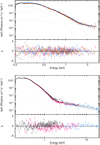 |
Fig. 9 Results of the phase-averaged spectral fitting. Top: we show the eROSITA spectra of detectors 2, 3, 4, and 6 simultaneously fit by the model of Table 6 and a fixed power-law index of Γ = 1.98. Bottom: simultaneous fit of eROSITA, XMM-Newton, and NuSTAR (dark gray, magenta, and blue data points, respectively). The best-fit parameters are listed in Table 6. |
3.2.2 Phase-resolved spectroscopy
The spin-resolved eROSITA spectra were first fit using a composite model (2BBPL) built from the combination of two bbodyrad components to model the thermal emission and a powerlaw component to take the nonthermal emission at higher energies into account. A interstellar absorption component was also taken into account. Similarly to the phase-averaged analysis, an edge and tbabs component were multiplied by the spectral model to take the feature around 0.26 keV into account, in accordance with the results of Sect. 3.2.1. We refer to this model as 2BBPLe; the ‘e’ indicates the inclusion of the new edge feature.
We set some model parameters to be the same for all phase-binned spectra: the interstellar absorption, the power-law slope, the temperatures of the two blackbody components, and the edge energy. Their best-fit values are listed in Table 7. In general, the resulting parameter values compare well to the spin phase-averaged fit results (Sect. 3.2.1), and the edge and photospheric parameters are not significantly sensitive to the power-law index.
We then performed fits including the Gaussian absorption line and refer to them as G2BBPL and G2BBPLe. All parameters of the Gaussian were allowed to vary freely. All the described models were initially applied to eROSITA data alone. The results for the nonvariable parameters are listed in the first four lines of Table 7. To improve the accuracy of the model parameters, we also conducted a simultaneous fit with eROSITA and XMM-Newton using the G2BBPLe model as well (third line in Table 7 and Fig. 11). This fit revealed indeed better constrained model parameters and a slightly lower photon index, but the best-fit values did not change much.
Similar to Fig. 8, the residuals of the fits with and without the phase-dependent Gaussian absorption line, as well as their bestfit parameters as given in the first two lines of Table 7, are shown as an apparent trailed spectrogram in Fig. 10 for eROSITA data alone. The fit without the absorption line shows strong residuals at energies between 0.5 keV and 0.6 keV in the phase interval between 0.8 and 1.4. The high  value indicates a poor choice of the null hypothesis. The fit with the Gaussian absorption line but without the edge has systematic residuals at 260 eV. The inclusion of both the Gaussian line and the edge reveals a statistically acceptable fit to the data. The two-dimensional spectrum of the residuals (lowest panel in Fig. 10) is compatible with pure statistical scatter.
We show the results regarding the phase-dependent parameters in Fig. 11. The variable parameters are the emitting areas and the parameters of the Gaussian absorption line. The radiation radii of the two blackbody components at infinity were computed assuming a distance of  pc. The radius values of the cold blackbody component (CBB) peak around phase 0.95, while the hot blackbody (HBB) radius values peak at phase 0.1, indicating a phase shift of 0.1–0.15 between the cold and hot thermal components.
As expected and known from the fit to the phase-averaged spectrum, the inclusion of the Gaussian absorption line has some effect on the temperature of the blackbodies and a strong effect on their normalization, hence emitting radius. The same is true for the edge, which mainly affects the cold blackbody temperature and hence its radius. Gaining a better understanding of the nature of the features is thus highly relevant for an understanding of the X-ray-to-ultraviolet SED, as discussed by Zharikov et al. (2021).
Fortunately, the parameters of the Gaussian line are only very weakly affected by the inclusion or the omission of the edge. Interestingly, the line parameters depend on the spin phase (see the bottom three panels of Fig. 11). The absorption is visible for about 60% of the spin cycle, centered on phase 0.1; it appears redshifted at the beginning and blueshifted at the end of its visibility interval. The same trend is observed in data from TM9 (not shown here), but shifted by 30–40 eV toward lower energies because of calibration uncertainties (Appendix D). In general terms, our analysis appears to reveal results that agree overall with the phase-resolved study performed by Arumugasamy et al. (2018, see their Fig. 15), although the fit strategy was somewhat different. The important difference is that the line parameters are more robustly determined with the new data we acquired and presented in this work.
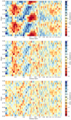 |
Fig. 10 Fit residuals from fitting the TM8 phase-resolved spectra using a 2BBPL (top), a G2BBPL (middle), or a G2BBPLe (bottom) model. |
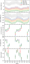 |
Fig. 11 Results for the phase-dependent parameters, estimated from the phase-resolved fit using a 2BBPL, 2BBPLe, G2BBPL, or G2BBPLe model. The errors are 1σ confidence levels. |
3.2.3 NS atmosphere and condensed surface models
The observed X-ray spectrum of PSR B0656+14 can be described with a phenomenological model, but the physical origin of the components that are thought to originate from the stellar surface remains largely unclear. X-ray pulsations and the derived blackbody parameters strongly suggest a nonuniform temperature distribution over the NS surface. They do not allow a quantitative interpretation of the observation because these estimates would be affected by the assumed temperature distribution and the fact that the local spectrum from a magnetized NS surface is known to deviate from a pure blackbody (see, e.g., Pavlov & Luna 2009; van Adelsberg et al. 2005). In this section we attempt to provide a more physically motivated description of the observed mean spectrum of PSR B0656+14. For comparison with the observed phase-averaged spectra, we computed models with a range of the angle γB between the magnetic dipole and the rotation axis and used this angle as one of the fit parameters. This is a strong simplification. This model does not predict pulsations. However, this approach will allow us to find the most promising model for further more sophisticated modeling.
The simplest model we applied is a cooling magnetized neutron star with a dipole surface magnetic field covered with a hydrogen atmosphere. We computed a grid of these models using the method that was recently employed to fit the thermal spectrum of PSR J1957+5033 by Zyuzin et al. (2021). We assumed that the mass and radius were fixed at M = 1.4 M⊙, R = 12 km and that the magnetic field strength at the magnetic pole was Bp = 1013 G. The grid parameter was the bolometric luminosity expressed through the redshifted effective temperature  , with log
  from 5.2 to 6.0 with a step of 0.1. The neutron star surface was divided into four latitude zones, one including the pole, and another the equator. For further details, see Zyuzin et al. (2021).
The computed grid of theoretical spectra, integrated over the neutron star surface for γB = 0°, 30°, 60°, and 90°, was used to fit the observed phase-averaged eROSITA spectrum (see Sect. 3.2.1). The best fit is presented in Fig. 12, and the obtained model parameters are listed in Table 8. The additional spectral components that were described above, a power law, a Gaussian absorption line, and an absorption edge, were also included because otherwise the model did not provide a statistically acceptable fit.
The obtained fit describes the observed spectral shape marginally well, although even with the inclusion of the additional components the quality of the fit is slightly lower than that provided by the phenomenological model. The more serious issue is, however, that the derived distance to the source (≈60 pc) is too small compared to the distance obtained from the radio-astrometric parallax,  pc (Brisken et al. 2003). In addition to the problem with the distance, the model does not provide a self-consistent description for the observed absorption line either. The same conclusions were obtained earlier by Arumugasamy et al. (2018) using various XSPEC spectral models describing the radiation of magnetized neutron star atmospheres.
To explain the observed absorption feature as proton cyclotron absorption, we considered the possibility that the magnetic field strength could be as high as B ~ 1014 G. Although the characteristic (spin-down) field is an order of magnitude lower, strong local fields at the surface cannot be excluded (cf. Tiengo et al. 2013; Mereghetti et al. 2015). A plasma envelope of magnetized neutron stars at this high field and at the temperature typical for the surface of PSR B0656+14 (kT ~ 0.1 keV) can be condensed (see, e.g., Taverna et al. 2020, their Fig. 1 and the related discussion). For this reason, we considered spectra of magnetized neutron stars with a condensed surface as an alternative physical model to describe the phase-averaged X-ray spectrum.
The emitting spectrum of the condensed surface can be computed using approaches suggested by Turolla et al. (2004) and van Adelsberg et al. (2005), but we used the analytic approximation for the iron-condensed surface (Potekhin et al. 2012). A spectrum of the condensed surface is close to a blackbody spectrum with two absorption features: one at the electron plasma energy Epe, and another extending from the ion cyclotron energy Ecyc,i to some upper energy  (see van Adelsberg et al. 2005, for details). The second feature is relatively narrow at high fields, and it can potentially describe the observed absorption line at 0.57 keV.
However, the integrated spectra of the magnetized neutron stars covered with the condensed surface are close to the single-blackbody spectra if a temperature distribution corresponding to the dipole field is assumed. As a result, these models cannot explain the observed spectrum, and temperature distributions more peaked to the poles have to be considered. These temperature distributions are possible if we introduce a strong toroidal component of the magnetic field in the crust (see, e.g. Pérez-Azorin et al. 2006; Suleimanov et al. 2010). In these models, most of the heat emerges near the magnetic poles, and the sizes of the polar hot spots depend on the relative contribution of the toroidal component. The temperature distribution is controlled by the related parameter aT according to the formulae given in the papers referenced above. If the toroidal component is negligible, aT ≈ 0.25, and aT increases with the enhanced toroidal component.
We developed a simple procedure introduced to XSPEC to fit X-ray spectra with the spectra of magnetized neutron stars with a condensed surface. We fit the observed phase-averaged eROSITA spectrum using the same methods and averaging procedure as described above. The best fit has a similar statistical significance as the previous attempt, see Fig. 12, and the best-fit parameters are also listed in Table 8, in the column labeled ‘CS’. The fit gives the necessary distance to the pulsar at the reasonable neutron star radius of about 12 km assuming aT ≈ 50. However, the depression between Ecyc,i and EC cannot completely describe the observed absorption line at 0.57 keV, and an additional Gaussian absorption line needs to be included to obtain an acceptable fit.
The third model that we applied to the eROSITA data includes the condensed surface and the model atmosphere. We assumed that the whole neutron star surface has a condensed surface, but the regions near magnetic poles with Bp ≈ 1014 G are covered with a thin hydrogen atmosphere with the column density Σ = 10 g cm−2. This atmosphere is optically thin at continuum photon energies, but it is optically thick near the proton cyclotron line. As a result, the emergent spectrum of the thin atmosphere is close to a blackbody with a proton cyclotron line, which can describe the observed absorption feature at 0.57 keV. This type of thin atmospheres was suggested for the X-ray dim isolated neutron stars (XDINS, or the so-called Magnificent Seven) by Ho et al. (2007), see also Suleimanov et al. (2010).
We computed seven models of thin magnetized hydrogen atmospheres with effective temperatures Teff between 1 MK and 2.2 MK with a step size of 0.2 MK and with a normal orientation of the magnetic field of strength B = 1014 G. Partial ionization of the atmosphere was taken into account. We used this grid of model spectra to fit the observed spectrum together with the model spectra of the neutron star covered with the condensed surface. The best fit is shown in Fig. 12 and the best-fit parameters are presented in Table 8, in the third column labeled ‘CS+Atm’. This fit does not require an additional Gaussian absorption line, but the physical interpretation of the model is ambiguous.
The global dipole magnetic field is comparable to the magnetic field strength derived from the observed spin-down, but the magnetic field in the hot spot described by the thin atmosphere is ten times larger. This may be explained by a complex structure of the field near the surface, with higher multipole components being much stronger than the dipole component. These models are widely discussed in view of the mounting body of observational and theoretical evidence that a complex field topology should be the rule rather than the exception (see, e.g., Viganò et al. 2021, and references therein). The thin hydrogen atmosphere can be the result of the nuclear spallation processes, which may present a self-regulating mechanism for producing a thin hydrogen atmosphere above a condensed iron surface (as suggested by Ho et al. 2007 in the case of RX J1856.5–3754). We note that the multicomponent field model with B ≈ 1014 G was also discussed by Arumugasamy et al. (2018).
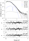 |
Fig. 12 Best fit of the averaged spectrum using three magnetized neutron star model spectra. (1) Covered by a hydrogen atmosphere (atm (pure)). (2) covered by an emitting condensed surface (CS (pure)). (3) Covered by an emitting condensed surface with an additional hot spot covered with a geometrically thin atmosphere (CS + atm; Σ = 10 g cm−2). See the detailed description in the text. The separate contributions of the components (CS (atm) and atm (CS)) are also shown. The deviations of each model from the observed spectrum are shown separately in the three bottom panels. |
Results of spectral fitting experiments using physically motivated models.
4 Discussion and conclusion
We have presented an in-depth analysis of a long, 100 ks, uninterrupted eROSITA observation of the nearby radio pulsar PSR B0656+14. This was the first eROSITA observation after the (longer than originally planned) commissioning phase performed with seven TMs of a stellar target. For cross-calibration purposes, the eROSITA observations were accompanied by simultaneous observations with XMM-Newton. Our analysis further benefits from the inclusion of archival NICER and NuSTAR data, the former for timing, the latter to better constrain the nonthermal emission. TM1 did not deliver science-grade data; for the spectral analysis, we only considered the detectors that were not affected by the optical leak (TM8).
We characterized the capabilities (and limitations) of eROSITA for timing studies of fast-spinning neutron stars such as PSR B0656+14 (spin period of 385 ms). Because this was performed at such an early phase of the mission, it was not possible to obtain an absolute time calibration of our observation. The relative timing accuracy was found to be about 5 × 10⁻⁷ s. Phase-folded light curves were eventually created using the eROSITA-determined period in various energy bands and found to be fully consistent with those from XMM-Newton, despite the much lower time resolution of eROSITA.
While addressing the question about the phase offset between the X-ray maximum and the radio pulse, we encountered unexpected timing uncertainties in the current radio ephemerides, despite their very high formal precision. We then established a new X-ray ephemeris based on two XMM-Newton and several NICER observations that covers the time interval from 2015 to 2020 with sufficient accuracy. Furthermore, we realized that the evolution of the X-ray pulse TOAs beyond the 2015 epoch was strong, which might be related to one or several glitches that had remained unnoticed so far. Our target is a well-known glitching pulsar (Espinoza et al. 2011), therefore this interpretation is perhaps likely. We did not establish the X-ray-to-radio phase relation, however, because we await further improvements of the ephemeris. In this regard, it will be extremely beneficial to have the involvement of the radio pulsar community in a joint analysis, for which we provide the necessary input data from the X-ray side here.
The main motivation for selecting PSR B0656+14 in the performance and verification phase of eROSITA was the tentative identification of an absorption feature at about 540 eV in a long XMM-Newton observation reported by Arumugasamy et al. (2018). The new observations add further knowledge about this feature. We first characterized the phase-averaged spectrum. The phenomenological model that we applied, which follows the description established by Arumugasamy et al. (2018), consists of two blackbody components, a hard power-law tail, and a superposed Gaussian at soft X-rays (G2BBPL). The Gaussian is highly significant and can be regarded as securely established. The parameters of the feature, its energy, ε ≃ 570 eV, and width, σ ≃ 70 eV, are revised and their accuracy improved.
Our modeling revealed an additional feature at soft energies, here described as an edge at about 260–265 eV, which may not be instrumental (model G2BBPLe). Zharikov et al. (2021) described a feature at ~0.3 keV when the analysis of XMM-Newton data was extended to energies below 0.3 keV. While their fit formally was clearly improved by inclusion of this additional line, they are cautious about its existence and seek for an independent detection with eROSITA. This paper presents the observational status of this feature for this particular star, and we are still cautious. In this regard, the analysis of additional observations of bright isolated neutron stars, namely the Magnificent Seven, performed by eROSITA on several occasions since launch, will hopefully settle the issue. If it is confirmed to be astronomical and not instrumental, it will reveal sought-for boundary conditions for future theoretical modeling of isolated neutron stars.
We presented three different types of model spectra and applied them to the multimission spectral data: a magnetized atmosphere, a condensed surface, and a mixed model. All three describe the shape of the continuum spectrum well, but only the last model spectrum provides some natural explanation for the occurrence of an absorption line.
The first model we tested was a semi-infinite atmosphere with temperature distributions corresponding to a dipole magnetic field. The model spectra resemble the observed spectrum at relatively low effective temperatures, implying a short distance to the star. If the X-ray emitting region were smaller than the whole stellar surface, the implied distance would even be smaller. The inapplicability of standard XSPEC neutron star atmosphere models was also reported by Arumugasamy et al. (2018).
If the magnetic field were much higher than 1013 G, other models would be suitable and were tested: a condensed surface, and a geometrically thin atmosphere. The local spectrum of the condensed surface is close to a blackbody spectrum. Therefore we need a special temperature distribution that mimics two blackbodies, a bright pole with a relatively cold rest surface, to obtain a reasonable spectral fit.
In the third model, the whole neutron star surface is covered by the condensed surface, and its radiation mimics that of the cold blackbody component in the phenomenological model. We then introduced the bright spot covered with the thin atmosphere. This second component mimics the hot black-body component in the two-blackbody fit. In addition, it contains the proton cyclotron line that explains the observed absorption feature, whose existence was definitely confirmed in this study (see the discussion of their tentatively identified feature by Arumugasamy et al. 2018).
In both cases of a pure condensed surface and the condensed surface plus thin atmosphere, the surface effective temperatures are significantly higher than for the semi-infinite atmospheres. Therefore the observed X-ray flux level can be provided by the neutron star at the pulsar distance of 288 pc. Our analysis of the phase-averaged spectrum is intended to test different physical models and possibly predetermine some of the spectral parameters. Construction of detailed, physically motivated fits to the phase-resolved spectra deserves a separate study, but this is beyond the scope of this paper.
The large number of photons that were collected with eROSITA allowed us to study the phase-dependent behavior of the main spectral parameters. The absorption line was traced through 60% of the spin cycle. This observation rules out an instrumental origin of the feature. The line is centered on phase 0.1 and shows 1σ variability of all its parameters: its location, width, and derived optical depth. Similarly, the behavior of the blackbody components was characterized through our phase-resolved spectroscopic study. The cold component reaches its maximum at phase ~0.9, whereas the hot component peaks at phase ~0.05. This behavior is clearly different from that described by De Luca et al. (2005), who reported an anticorrelation of the radii of the cold and hot blackbody components. The higher statistics obtained with the deep XMM-Newton and eROSITA observations clearly establish a more complex picture. The absolute value of the blackbody radii (not their phase relation) is strongly dependent on the inclusion of the absorption line at 570 eV in the modeling. The nature of this absorption line remains uncertain, however. Difficulties in achieving a unique interpretation arise from complex temperature distributions over the stellar surface and corresponding kinks in the continuum spectra (e.g., Viganò et al. 2014), from calibration uncertainties, from uncertainties of the correct spectral model, and from the limited energy coverage of the spectra.
Despite these difficulties, a few important constraints can be derived regarding the location in which this line originates. Is it far (magnetospheric) or near (atmospheric)? The line is seen only for ~60%, which is perhaps simpler to understand if it were near (h ≪ RNS). However, Tiengo et al. (2013) discussed a possible far location (R ~ 3RNS) of the absorber in the magnetar SGR 0418 + 5729 to explain the phase-variable absorption feature. If this is applied to our target, the implied magnetic field strength from the proton cyclotron interpretation would not inform about the field at the surface, which would be significantly higher and in the magnetar regime. Observationally, the line visibility is centered on phase 0.1, that is, it coincides in phase with the maximum of the hot blackbody-emitting region. A direct relation between the two might be speculated about. This is premature, however. The hot blackbody is seen at all phases, its emitting radius varies by ~30% only, but the absorption line is clearly constrained in phase. In this regard, it is instructive to consider Figs. 3 and 4 of Beloborodov (2002), who sketched visibility periods and light curve shapes of blackbody pulse profiles as a function of the inclination i of the spin axis and the spot latitude θ. The light curve of the hot blackbody resembles their class I, that is, a combination of moderately high values of both angles. The ‘light curve’ (here visibility curve) of the absorption feature resembles their class II, which would imply a higher spot latitude than the blackbody for a given inclination. Hence the hot blackbody and the absorption like are likely spatially disjunct despite the similarities in their phase dependence.
Phase-resolved light curves for photon energies below ~2 keV were established with very high signal-to-noise ratio. At energies below 0.7 keV, they are highly asymmetric and might be indicative of a third spot or a more complex temperature distribution over the surface of the star. This might be modeled using MEM-inversion techniques similar as for mapping spots on active stars (e.g., Berdyugina et al. 2002) when a better understanding of the continuum emission processes is achieved. These studies will also benefit from the larger body of eROSITA observations of XDINS (Pires et al., in prep.).
Evidence for narrow absorption features at similar energies was reported in the RGS spectra of several thermally emitting isolated neutron stars (see Hambaryan et al. 2009; Hohle et al. 2012, and references therein), but the interpretation remains unclear. In particular, the analysis of Pires et al. (2019) of the nearby XDINS RX J1605.3+3249, based on a recent XMM-Newton large program and on archival RGS observations of the source extending back to 2002, revealed that evidence for the line is only found in the early observations. For PSR B0656+14, we found weak evidence for a line in the RGS spectra alone, its energy and parameters are consistent with those found in eROSITA and pn data, however.
Acknowledgements
Support of this work by the German DLR under contracts 50 QR 1604, 50 QR 2104 and 50 OX 1901 is gratefully acknowledged. A.M.P. gratefully acknowledges support from the Chinese Academy of Science’s President International Fellowship Initiative (CAS PIFI 2019VMC0008). V.S. thanks the Deutsche Forschungsgemeinschaft (DFG) for financial support (grant WE 1312/53-1). His work has also been supported by the grant 14.W03.31.0021 of the Ministry of Science and Higher Education of the Russian Federation. The work of A.Y.P. was partially supported by the Russian Foundation for Basic Research (RFBR) according to the research project 19-52-12013. We thank the XMM-Newton project scientist, Dr. Norbert Schartel, for the generous allocation of observation time and the ESAC-SOC for simultaneous scheduling of the observations. We thank Chris Flynn, Matthew Bailes and Marcus Lower from the Swinburne University of Technology for communicating their latest ephemeris for B0656+14 prior to publication. This work is based on data from eROSITA, the primary instrument aboard SRG, a joint Russian-German science mission supported by the Russian Space Agency (Roskosmos), in the interests of the Russian Academy of Sciences represented by its Space Research Institute (IKI), and the Deutsches Zentrum für Luft- und Raumfahrt (DLR). The SRG spacecraft was built by Lavochkin Association (NPOL) and its subcontractors, and is operated by NPOL with support from the Max Planck Institute for Extraterrestrial Physics (MPE). The development and construction of the eROSITA X-ray instrument was led by MPE, with contributions from the Dr. Karl Remeis Observatory Bamberg & ECAP (FAU Erlangen-Nuernberg), the University of Hamburg Observatory, the Leibniz Institute for Astrophysics Potsdam (AIP), and the Institute for Astronomy and Astrophysics of the University of Tübingen, with the support of DLR and the Max Planck Society. The Argelander Institute for Astronomy of the University of Bonn and the Ludwig Maximilians Universität Munich also participated in the science preparation for ero. The eROSITA data shown here were processed using the eSASS/NRTA software system developed by the German eROSITA consortium.
Appendix A TM1 malfunction
The anomalous behavior of TM1 was noted early and could not be fixed during the various pipeline processing stages of this observation, which took calibration updates and ever improved software versions into account. In the most recent processing (version c001) that enters the public area, the overall number of photons in TM1 was only about 60% of that in the other cameras, a coarsely binned light curve (50 s bin size) in original time sequence was much noisier than for the other TMs and showed a low-frequency modulation of the mean rate, and a GTI-filtered light curve contained no photons at all. The reason for the malfunction of TM1 during this observation is not known. We excluded the data from TM1 from the scientific analysis presented in this paper.
Appendix B Time system of SRG and eROSITA
NPOL/Lavochkin in cooperation with Roscosmos operates the SRG spacecraft and controls the central spacecraft clock via radar signals. These measurements are performed routinely since November 3, 2019, hence almost three weeks after the observations of B0656, with the simple consequence that an absolute value for the photon arrival times of the pulsar as observed with SRG/eROSITA cannot be given. Time shifts are applied to the central spacecraft clock due to some instability of the central quartz. The size of it and the possible effect on our observations are described here.
When the offsets between UTC and OBT (onboard time) reach a limit of 1 s, time shifts are applied to keep the offsets always between 0 and 1 s. The history of these shifts in the time interval between launch and end of 2020 is documented in Table B.1. The offset history corrected for the time shifts is shown in Fig. B.1. For data representation and polynomial fits applied to the data, the time axis was renormalized to 0 at MJD 59000. Time offset errors were assumed to be 0.002 s before MJD 59100 and 0.0005 s after that date. These values were estimated by us from the scatter of the daily measured clock drift. A linear fit to the measured drift (upper graph in Fig. B.1) does not provide an acceptable representation of the data. Only a cubic fit applied to the data leaves mainly scatter in the O–C residuals (shown in the lower panels of the two graphs). In the context of the current paper, only the linear term is relevant, which is 0.0119660(5) s d−1, and 0.011933(1) s d−1 for the two fits we show.
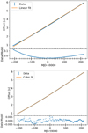 |
Fig. B.1 Linear and cubic fits to the accumulated offsets between UTC and the spacecraft clock. |
Time-shift history of the SRG quartz.
Appendix C X-ray ephemeris based on NICER and XMM-Newton data
In Table C.1, we list some of the relevant parameters extracted from the parameter files describing the available timing solutions. The values from Lower et al. were made kindly available to us prior to publication.
Ephemeris parameter files (abridged) used in this paper.
In Table C.2, we list the NICER (abbreviation NI) and XMM-Newton (abbreviation X) observations (identified with the abbreviations NI or X followed by the respective observation ID) and the derived pulse arrival time that were used to determine the X-ray ephemeris of Sect. 3.1.1.
Summary of observations and TOAs for the pulsar ephemeris.
Mean best-fit parameters and percentage deviation according to eROSITA detector type and pattern.
Appendix D Cross-calibration of the eROSITA detectors
For cross-calibration purposes, we performed simple fits of the phenomenological model discussed in Sect. 3.2.1 to the spectra of PSR B0656+14 in each of the six TMs. The same analysis and fitting procedure as described in Sect. 3.2.1 were applied here. In Table C.3 we list the mean results over eROSITA detector type (with and without on-chip filter) and for various pattern combinations (s, d, and sdtq). The average percentage deviation from the mean values is also listed for the two detector groups. For a given pattern, these are typically smaller for TMs 5 and 7, while a larger dispersion of the best-fit parameters is consistently observed for doubles in both groups. The lower fit quality (higher chi-square values) is obtained for the detectors affected by the optical light leak (TMs 5 and 7). The largest inconsistencies between patterns are observed for the parameters of the Gaussian absorption and the overall model flux of detectors 5 and 7.
In Table D.1, we compare the results of a single stacked spectra, extracted from the concatenated TM8 and TM9 event files, with those where, according to detector type, 5 and 2 individual detector data sets are fit simultaneously in XSPEC. These results are labeled TM2346 and TM57 in Table D.1; no filtering in photon pattern is applied. Similarly, we show the results of TM0 against TM234567 and TM89 (6 and 2 data sets, respectively). Whenever the data sets were fit simultaneously, we allowed for a renormalization factor in XSPEC to account for calibration uncertainties between the instruments. The strength of the edge component in each data set was also allowed to vary independently. As usual, the source and background spectra of the stacked data sets, as well as the ancillary and response files, were produced with the eSASS task srctool. As a reference for the best-fit parameters (but without the edge component), the fit results of the simultaneous fit of the two EPIC-pn data sets described in Sects. 2.2 and 3.2.1 are also shown in Table D.1.
Cross-calibration of the two different types of eROSITA detectors.
Clearly, the two types of eROSITA instrument converge to different fit solutions. In particular, the best-fit blackbody temperatures of the TM8 data sets agree with pn within 1.1–6%, whereas it is 10-16% lower for the data sets without the on-chip filter. This is likely due to the altered energy scale of these two detectors as a result of the optical leak (Sect. 2). The parameters of the edge component are also remarkably inconsistent: the edge is detected at a 20% lower energy and at much higher optical depth in TM9 than in TM8. This argues against stacking the two detector types into a single data set because it may bias the parameter estimation (i.e., the fit does not necessarily converge to an average solution). On the other hand, the analysis shows that the adoption of TM8 or TM9 instead of the corresponding data sets 2, 3, and 4, and 6, 5, and 7 produces results that are completely consistent within the errors. Moreover, the fit results of Table D.1 agree well with the mean parameters of Table C.3, as expected.
References
- Arnaud, K. A. 1996, in Astronomical Data Analysis Software and Systems V, eds. G. H. Jacoby, & J. Barnes, ASP Conf. Ser., 101, 17 [Google Scholar]
- Arumugasamy, P., Kargaltsev, O., Posselt, B., Pavlov, G. G., & Hare, J. 2018, ApJ, 869, 97 [NASA ADS] [CrossRef] [Google Scholar]
- Becker, W., & Trümper, J. 1997, A&A, 326, 682 [NASA ADS] [Google Scholar]
- Beloborodov, A. M. 2002, ApJ, 566, L85 [Google Scholar]
- Berdyugina, S. V., Pelt, J., & Tuominen, I. 2002, A&A, 394, 505 [NASA ADS] [CrossRef] [EDP Sciences] [Google Scholar]
- Brisken, W. F., Thorsett, S. E., Golden, A., & Goss, W. M. 2003, ApJ, 593, L89 [NASA ADS] [CrossRef] [Google Scholar]
- Brunner, H., Liu, T., Lamer, G., et al. 2022, A&A, 661, A1 (eROSITA EDR SI) [NASA ADS] [CrossRef] [EDP Sciences] [Google Scholar]
- Buccheri, R., Bennett, K., Bignami, G. F., et al. 1983, A&A, 128, 245 [NASA ADS] [Google Scholar]
- Buchner, J. 2014, ArXiv e-prints, [arXiv:1487.5459] [Google Scholar]
- Buchner, J. 2017, ArXiv e-prints, [arXiv:1787.84476] [Google Scholar]
- De Luca, A., & Molendi, S. 2004, A&A, 419, 837 [NASA ADS] [CrossRef] [EDP Sciences] [Google Scholar]
- De Luca, A., Caraveo, P. A., Mereghetti, S., Negroni, M., & Bignami, G. F. 2005, ApJ, 623, 1051 [NASA ADS] [CrossRef] [Google Scholar]
- Espinoza, C. M., Lyne, A. G., Stappers, B. W., & Kramer, M. 2011, MNRAS, 414, 1679 [NASA ADS] [CrossRef] [Google Scholar]
- Fisher, R., Bennett, J., & Yates, F. 1990, Statistical Methods, Experimental Design, and Scientific Inference (OUP Oxford) [Google Scholar]
- Greiveldinger, C., Camerini, U., Fry, W., et al. 1996, ApJ, 465, L35 [NASA ADS] [CrossRef] [Google Scholar]
- Hambaryan, V., Neuhäuser, R., Haberl, F., Hohle, M. M., & Schwope, A. D. 2009, A&A, 497, L9 [NASA ADS] [CrossRef] [EDP Sciences] [Google Scholar]
- Harding, A., Enoto, T., Kobayaashi, S., et al. 2019, in AAS/High Energy Astrophysics Division, 17, AAS/High Energy Astrophysics Division, 111.10 [NASA ADS] [Google Scholar]
- Ho, W. C. G., Kaplan, D. L., Chang, P., van Adelsberg, M., & Potekhin, A. Y. 2007, MNRAS, 375, 821 [CrossRef] [Google Scholar]
- Hohle, M. M., Haberl, F., Vink, J., de Vries, C. P., & Neuhäuser, R. 2012, MNRAS, 419, 1525 [CrossRef] [Google Scholar]
- Huppenkothen, D., Bachetti, M., Stevens, A. L., et al. 2019, ApJ, 881, 39 [Google Scholar]
- Johnston, S., & Kerr, M. 2018, MNRAS, 474, 4629 [NASA ADS] [CrossRef] [Google Scholar]
- Liu, T., Merloni, A., Comparat, J., et al. 2022, A&A, 661, A27 (eROSITA EDR SI) [NASA ADS] [CrossRef] [EDP Sciences] [Google Scholar]
- Lower, M. E., Bailes, M., Shannon, R. M., et al. 2020, MNRAS, 494, 228 [CrossRef] [Google Scholar]
- Marshall, H. L., & Schulz, N. S. 2002, ApJ, 574, 377 [NASA ADS] [CrossRef] [Google Scholar]
- Mereghetti, S., Pons, J. A., & Melatos, A. 2015, Space Sci. Rev., 191, 315 [NASA ADS] [CrossRef] [Google Scholar]
- Pavlov, G. G., & Luna, G. J. M. 2009, ApJ, 703, 910 [NASA ADS] [CrossRef] [Google Scholar]
- Pavlov, G. G., Zavlin, V. E., & Sanwal, D. 2002, in Neutron Stars, Pulsars, and Supernova Remnants, eds. W. Becker, H. Lesch, & J. Trümper, 273 [Google Scholar]
- Pérez-Azorín, J. F., Miralles, J. A., & Pons, J. A. 2006, A&A, 451, 1009 [NASA ADS] [CrossRef] [EDP Sciences] [Google Scholar]
- Pires, A. M., Schwope, A. D., Haberl, F., et al. 2019, A&A, 623, A73 [NASA ADS] [CrossRef] [EDP Sciences] [Google Scholar]
- Possenti, A., Mereghetti, S., & Colpi, M. 1996, A&A, 313, 565 [NASA ADS] [Google Scholar]
- Potekhin, A. Y., Suleimanov, V. F., van Adelsberg, M., & Werner, K. 2012, A&A, 546, A121 [NASA ADS] [CrossRef] [EDP Sciences] [Google Scholar]
- Predehl, P., Andritschke, R., Arefiev, V., et al. 2021, A&A, 647, A1 [EDP Sciences] [Google Scholar]
- Ray, P. S., Kerr, M., Parent, D., et al. 2011, ApJS, 194, 17 [NASA ADS] [CrossRef] [Google Scholar]
- Suleimanov, V., Hambaryan, V., Potekhin, A. Y., et al. 2010, A&A, 522, A111 [NASA ADS] [CrossRef] [EDP Sciences] [Google Scholar]
- Taverna, R., Turolla, R., Suleimanov, V., Potekhin, A. Y., & Zane, S. 2020, MNRAS, 492, 5057 [NASA ADS] [CrossRef] [Google Scholar]
- Tiengo, A., Esposito, P., Mereghetti, S., et al. 2013, Nature, 500, 312 [CrossRef] [Google Scholar]
- Turolla, R., Zane, S., & Drake, J. J. 2004, ApJ, 603, 265 [NASA ADS] [CrossRef] [Google Scholar]
- van Adelsberg, M., Lai, D., Potekhin, A. Y., & Arras, P. 2005, ApJ, 628, 902 [NASA ADS] [CrossRef] [Google Scholar]
- Viganò, D., Perna, R., Rea, N., & Pons, J. A. 2014, MNRAS, 443, 31 [CrossRef] [Google Scholar]
- Viganò, D., Garcia-Garcia, A., Pons, J. A., Dehman, C., & Graber, V. 2021, Comput. Phys. Commun., 265, 108001 [CrossRef] [Google Scholar]
- Wilms, J., Allen, A., & McCray, R. 2000, ApJ, 542, 914 [Google Scholar]
- Zharikov, S., Zyuzin, D., Shibanov, Y., et al. 2021, MNRAS, 502, 2005 [NASA ADS] [CrossRef] [Google Scholar]
- Zyuzin, D. A., Karpova, A. V., Shibanov, Y. A., Potekhin, A. Y., & Suleimanov, V. F. 2021, MNRAS, 501, 4998 [CrossRef] [Google Scholar]
For a description of the eSASS tasks and algorithms, see Brunner et al. (2022).
Specifically, we removed objects with an extent parameter larger than 70″ from the source list that were detected up to 5′ away from the pulsar position.
Specifically, we added “LOCAL” and “ICRS” to the TIMEREF and RADECSYS keywords.
We gratefully acknowledge the use of the Lower et al. updated parameter file, which includes data from the UTMOST program prior to publication.
In XSPEC, tbabs((bbodyrad+bbodyrad+powerlaw)gabs)edge, cf. fit IDs [i, ii, iii] in Table 6.
Because of the defective channels of RGS2 around the wavelength range of interest, the RGS2 spectrum cannot constrain the presence of the narrow line.
All Tables
Joint and supporting SRG/eROSITA, XMM-Newton, and NuSTAR observations of PSR B0656+14.
Pulsed fractions (pf) and phases of pulse maxima (φmax) in different energy bands for the 2019 eROSITA/XMM-Newton campaign.
Mean best-fit parameters and percentage deviation according to eROSITA detector type and pattern.
All Figures
|
Fig. 1 Composite eROSITA image produced from selected photons in three different energy bands (red: 0.2–0.5 keV, green: 0.5–1.5 keV, and blue: 1.5–7 keV) showing the large eROSITA field of view. The pulsar B0656 is centrally located at the aimpoint. The white rectangle shows the field of view of the XMM-Newton observations that were simultaneously conducted with EPIC-pn in the small-window mode. |
| In the text | |
|
Fig. 2 Extraction regions we adopted in the analysis. The source and background regions are centered at right ascension 104.951117 deg and declination +14.239175 deg. The exclusion zones of contaminants are shown as cyan circles with a red bar. Left. source extraction radius (yellow) of 150″ (TM2; 0.2–10 keV). Right. background annulus (magenta) has inner and outer radii 10′ and 15′, respectively (TM6; 0.2–10 keV). |
| In the text | |
|
Fig. 3 Distribution of photon pattern fractions as a function of energy. The observed fractions of singles (s), doubles (d), singles and doubles (s + d), triples (t), and quadruples (q) are shown as data points for the TM8 detector combination. Solid lines show the expected (theoretical) pattern distribution in the 0.2–2 keV energy band. |
| In the text | |
|
Fig. 4 XMM-Newton SW observation of PSR B0656+14, performed simultaneously with eROSITA in October 2019. Source and background extraction regions are overlaid (blue circle with radius 22.5″ and green boxes of sizes 110″ × 58″ (left)and 44″ × 50″ (right); 0.3–12 keV). The image has 63 × 64 pixels, about 4.3 × 4.3′. |
| In the text | |
|
Fig. 5 Period search of eROSITA and XMM-Newton data. |
| In the text | |
|
Fig. 6 Phaseograms showing pulse proflies in 0.3–2 keV for individual data groups listed in Table C.2 folded using Johnston & Kerr (2018) (left) and the updated ephemeris (middle) obtained in this work. The phase residuals to the best-fit solution (black symbols with error bars) and for the Johnston & Kerr (2018) solution (red, zerophase corresponds to the phase of the radio peak, and errors are omitted for clarity) are also shown in the right panel. |
| In the text | |
|
Fig. 7 Background-subtracted eROSITA and XMM-Newton pulse profile in different energy bands. The original data were averaged into 20 phase bins at soft and medium energies and averaged into 10 phase bins at hard energies. The light curves are shifted to a common phase, where phase zero is defined as the maximum of the main pulse (see the text for details). |
| In the text | |
|
Fig. 8 Trailed spectrogram of the eROSITA pulse profile, with phase and energy along the y– and x–axes, respectively. The mean spectrum was subtracted from the original data. Color thus indicates a positive or negative deviation from the mean. Excess values were normalized to their errors. The pulse profile is shown twice for better visibility. |
| In the text | |
|
Fig. 9 Results of the phase-averaged spectral fitting. Top: we show the eROSITA spectra of detectors 2, 3, 4, and 6 simultaneously fit by the model of Table 6 and a fixed power-law index of Γ = 1.98. Bottom: simultaneous fit of eROSITA, XMM-Newton, and NuSTAR (dark gray, magenta, and blue data points, respectively). The best-fit parameters are listed in Table 6. |
| In the text | |
|
Fig. 10 Fit residuals from fitting the TM8 phase-resolved spectra using a 2BBPL (top), a G2BBPL (middle), or a G2BBPLe (bottom) model. |
| In the text | |
|
Fig. 11 Results for the phase-dependent parameters, estimated from the phase-resolved fit using a 2BBPL, 2BBPLe, G2BBPL, or G2BBPLe model. The errors are 1σ confidence levels. |
| In the text | |
|
Fig. 12 Best fit of the averaged spectrum using three magnetized neutron star model spectra. (1) Covered by a hydrogen atmosphere (atm (pure)). (2) covered by an emitting condensed surface (CS (pure)). (3) Covered by an emitting condensed surface with an additional hot spot covered with a geometrically thin atmosphere (CS + atm; Σ = 10 g cm−2). See the detailed description in the text. The separate contributions of the components (CS (atm) and atm (CS)) are also shown. The deviations of each model from the observed spectrum are shown separately in the three bottom panels. |
| In the text | |
|
Fig. B.1 Linear and cubic fits to the accumulated offsets between UTC and the spacecraft clock. |
| In the text | |
Current usage metrics show cumulative count of Article Views (full-text article views including HTML views, PDF and ePub downloads, according to the available data) and Abstracts Views on Vision4Press platform.
Data correspond to usage on the plateform after 2015. The current usage metrics is available 48-96 hours after online publication and is updated daily on week days.
Initial download of the metrics may take a while.