| Issue |
A&A
Volume 661, May 2022
The Early Data Release of eROSITA and Mikhail Pavlinsky ART-XC on the SRG mission
|
|
|---|---|---|
| Article Number | A23 | |
| Number of page(s) | 11 | |
| Section | Planets and planetary systems | |
| DOI | https://doi.org/10.1051/0004-6361/202141097 | |
| Published online | 18 May 2022 | |
Exoplanet X-ray irradiation and evaporation rates with eROSITA★
1
Leibniz Institute for Astrophysics Potsdam,
An der Sternwarte 16,
14482
Potsdam,
Germany
e-mail: This email address is being protected from spambots. You need JavaScript enabled to view it.
2
Potsdam University, Institute for Physics and Astronomy,
Karl-Liebknecht-Straße 24/25,
14476
Potsdam,
Germany
Received:
15
April
2021
Accepted:
21
June
2021
Abstract
High-energy irradiation is a driver for atmospheric evaporation and mass loss in exoplanets. This work is based on data from eROSITA, the soft X-ray instrument on board the Spectrum Roentgen Gamma mission, as well as on archival data from other missions. We aim to characterise the high-energy environment of known exoplanets and estimate their mass-loss rates. We use X-ray source catalogues from eROSITA, XMM-Newton, Chandra, and ROSAT to derive X-ray luminosities of exoplanet host stars in the 0.2–2 keV energy band with an underlying coronal, that is, optically thin thermal spectrum. We present a catalogue of stellar X-ray and EUV luminosities, exoplanetary X-ray and EUV irradiation fluxes, and estimated mass-loss rates for a total of 287 exoplanets, 96 of which are characterised for the first time based on new eROSITA detections. We identify 14 first-time X-ray detections of transiting exoplanets that are subject to irradiation levels known to cause observable evaporation signatures in other exoplanets. This makes them suitable targets for follow-up observations.
Key words: stars: coronae / stars: activity / planet-star interactions / planets and satellites: atmospheres / X-rays: stars
Full Table B.1 is only available at the CDS via anonymous ftp to cdsarc.u-strasbg.fr (130.79.128.5) or via http://cdsarc.u-strasbg.fr/viz-bin/cat/J/A+A/661/A23
© ESO 2022
1 Introduction
Exoplanets have been detected in a wide variety of orbital architectures, and a significant fraction of them orbit their host stars at close orbital distances. The first exoplanet detected around a main-sequence star, 51 Peg b, is an example of a so-called hot Jupiter, orbiting its host star in only 4.2 days (Mayor & Queloz 1995). Exoplanets in close orbits are subject to much higher levels of irradiation from the host star than any planets in our own Solar System. The intense irradiation across the electromagnetic spectrum can cause inflated radii of hot Jupiters (see Fortney & Nettelmann 2010; Baraffe et al. 2010 for reviews). In the UV and X-ray part of the spectrum, the stellar photons are absorbed at high altitudes in the exoplanetary atmosphere, where they can power a hydrodynamic evaporation process (Watson et al. 1981; Murray-Clay et al. 2009). Extended exoplanetary atmospheres as well as ongoing atmospheric escape have been detected through different observational setups that target certain parts of the spectrum in which even optically thin atmospheric layers can cause enough absorption of starlight to produce observational effects during exoplanetary transits. Examples are the Lyman-α line of hydrogen (Vidal-Madjar et al. 2003; Lecavelier Des Etangs et al. 2010; Kulow et al. 2014; Ehrenreich et al. 2015), the near-infrared metastable lines of helium (Spake et al. 2018; Nortmann et al. 2018), and observations in the near-ultraviolet (Salz et al. 2019) and in soft X-rays (Poppenhaeger et al. 2013).
The main driver for exoplanetary atmospheric escape is thought to be the extreme-ultraviolet (EUV) and soft X-ray flux that the planet receives from the host star (Yelle 2004; Murray-Clay et al. 2009). The EUV component of the stellar spectrum is currently not directly observable because no space observatories with sensitivity at the corresponding wavelengths are in operation; the EUVE satellite was the last major EUV observatory and ceased operations in 2001. In contrast, the X-ray part of the stellar spectrum is observable with a variety of currently operating instruments. The stellar EUV flux in turn can be estimated from the stellar X-ray emission and the UV part of the stellar spectrum (Sanz-Forcada et al. 2011; France et al. 2013). Several uncertainties still exist when the mass-loss rates of exoplanets are estimated, for example the X-ray absorption height in exoplanetary atmospheres and the overall efficiency of exoplanetary mass loss (Owen & Adams 2014; Cohen et al. 2015; Dong et al. 2017), or mass-loss effects on planet-formation in protoplanetary disks (Monsch et al. 2019). However, one of the most important input quantities of exoplanet evaporation rates, namely the exoplanetary high-energy irradiation, can be determined through X-ray observations.
Launched in 2019, eROSITA is producing the first all-sky survey in X-rays since the ROSAT mission in the 1990s. We present a catalogue of exoplanet X-ray irradiation levels derived from the eROSITA full-sky survey data and the eROSITA Final Equatorial Depth Survey (eFEDS; see Brunner et al. 2022), augmented by archival observations from ROSAT, XMM-Newton, and Chandra. We calculate the stellar combined X-ray and EUV (in short, XUV) fluxes as well as estimates for the exoplanetary evaporation rates. We report on several exoplanets that are strongly irradiated in the high-energy regime, which makes them good candidates for observing ongoing evaporation signatures at other wavelengths.
The paper is structured as follows: Sect. 2 describes the observations and data reduction; Sect. 3 describes the considerations we used for the catalogue matching and the analysis we performed to extract flux estimates for stellar coronae; Sect. 4 gives the main results with respect to stellar X-ray fluxes and luminosities, exoplanetary irradiation levels, and mass-loss rates; Sect. 5 places the results in the context of exoplanet evaporation; and Sect. 6 summarises our findings.
2 Observations
2.1 eROSITA
The eROSITA instrument consists of seven X-ray telescopes and CCD cameras on board the Russian–German Spectrum-X-Gamma (SRG) spacecraft (Sunyaev et al. 2021) and was launched into orbit in summer 2019. A detailed description of eROSITA is given in Merloni et al. (2012) and Predehl et al. (2021). In short, eROSITA has a circular field of view with a diameter of 1.03°, an average spatial resolution of 26″, and is sensitive to photons from an energy range of 0.2–10 keV. eROSITA observes the whole sky once within six months by scanning along great circles in the sky that are approximately perpendicular to the ecliptic, similar to the ROSAT All-Sky Survey (Voges et al. 1999, 2000; Boller et al. 2016). The survey portion of the eROSITA mission, called the eROSITA All-Sky Survey (eRASS), will last 4 yr, in which the whole sky is scanned eight times. Prior to starting the eRASS, eROSITA performed a calibration and performance verification phase (CalPV), in which it observed an equatorial field of about 140 deg2 size for an average exposure time of ca. 2 ks per pixel, in order to image a small patch of the sky to the same depth as is expected at the end of the 4-yr all-sky survey. This eROSITA Final Equatorial Depth Survey (eFEDS) (Brunner et al. 2022) will be included in the Early Data Release of the eROSITA consortium in 2021.
We used data from the intermediate consortium-wide data release of the eRASS1 and eRASS2 surveys, meaning the first and second full-sky surveys performed by eROSITA. We have access to all eRASS X-ray sources located in the half of the sky, which is proprietary to eROSITA_DE, the German eROSITA collaboration (i.e. with a galactic longitude higher than 180°). The raw data were processed with a calibration pipeline based on the eROSITA Science Analysis Software System (eSASS) (see Brunner et al. 2022). The intermediate eRASS1 and eRASS2 catalogues list the positions, detection likelihoods, and vignetting-corrected count rates of the detected X-ray sources in three energy bands, 0.2–0.6 keV, 0.6–2.3 keV, and 2.3–5.0 keV, among other parameters. Typical vignetting-corrected exposure times over an individual half-year survey are about 150 seconds per source, but can differ strongly depending on the position of the source on the sky, with longer exposure times towards the ecliptic poles.
For stellar coronae, significant X-ray emission is typically found at energies below 5 keV, with the exception of extremely powerful (but transient) flares (see Güdel 2004 for a review). We therefore concentrate our study on the three canonically extracted energy bands (0.2–0.6,0.6–2.3 and 2.3–5.0 keV) of the intermediate eRASS catalogues.
2.2 ROSAT
ROSAT was a space telescope that observed the sky in soft X-rays in an energy range of 0.1–2.4 keV (Truemper 1982), with an all-sky survey (RASS) as well as pointed observations. We used the Second ROSAT all-sky survey (2RXS) source catalogue from Boller et al. (2016), which is available through the VizieR service. To obtain stellar coronal fluxes, we used the counts-to-flux conversion formula from Schmitt et al. (1995), which uses detected count rates and hardness ratios from RASS for a flux calculation. We later scaled these fluxes to a canonical energy band of 0.2–2keV, with details given in Sect. 3.2.
2.3 XMM-Newton
XMM-Newton is an X-ray mission with several instruments on board (Jansen et al. 2001). Relevant for our analysis here are only the data collected by the EPIC instrument, consisting of three CCD cameras (Turner et al. 2001; Strüder et al. 2001). The energy range and spatial resolution of EPIC is similar to that of eROSITA. The XMM-Newton mission provides a number of different source catalogues, including merged source detections from pointed observations, the slew survey, and multiply observed sources (see e.g. Saxton et al. 2008; Watson et al. 2009; Traulsen et al. 2020). We used the 4XMM-DR10 catalogue1 in its slim version, where the longest existing exposure was selected for any given source.
2.4 Chandra
Chandra is an X-ray telescope with two X-ray imaging instruments, ACIS and HRC (Weisskopf et al. 2002; Garmire et al. 2003; Murray et al. 1997). HRC is sensitive to photon energies from 0.08 to 10.0 keV, but provides no intrinsic energy resolution. ACIS has an intrinsic energy resolution of 50 eV (full width at half maximum, FWHM) at soft energies, and has an energy sensitivity of 0.2–10.0 or 0.6–10.0 keV, depending on which chip of the ACIS instrument a source falls onto. We used the Chandra Source Catalog (CSC), Release 2.0 (Evans et al. 2010; Evans & Civano 2018) for our analysis, which is available through the VizieR interface.
3 Data analysis
3.1 Catalogue cross-matching
We used the NASA Exoplanet Archive catalogue of detected exo-planets as our starting point. We downloaded the full table of confirmed exoplanets and their properties on March 26, 20212, using their default data sets for each exoplanet. We excluded the small number of exoplanets detected by the microlensing method because their stellar distances have large uncertainties of about 50%, which would propagate into our final exoplanetary mass-loss rates as very large uncertainties. We also discarded one entry in the exoplanet table, namely the postulated exoplanet around the cataclysmic variable HU Aqr, because the planet has been shown to be spurious (Schwope & Thinius 2014; Bours et al. 2014; Goździewski et al. 2015). We plot the remaining exoplanets from the catalogue as the grey points in Fig. 1.
The host star coordinates in the Exoplanet Archive table are based on optical observations and are given by NASA for epoch J2015.5 for all sources with a Gaia DR2 source ID (Gaia Collaboration 2018; Lindegren et al. 2018), and for epoch J2000 for the remaining few exoplanet host stars without a Gaia DR2 entry. We propagated all host star coordinates to epochs suitable for catalogue matching with the respective X-ray catalogues, using the Gaia DR2 proper motions where available, and HIPPARCOS proper motions otherwise. Typical proper motions of known exoplanet host stars within a distance of 100 pc from the Sun are about 200 µarcsec yr−1 and significantly smaller at larger distances, but a small number of stars in the sample display proper motions upwards of 1 arcsec yr−1.
We then performed a positional source matching of the exoplanet catalogue with the individual X-ray catalogues. The closest X-ray source in a chosen matching radius to an exoplanet host star was selected as the fiducial match. Maximum matching radii were based on considerations of both the typical positional uncertainties of the respective telescopes and the expected uncertainties in propagated stellar positions at the observing epoch. The typical positional uncertainties of the X-ray catalogues are about 12.5″ for ROSAT (Voges et al. 1999), 1.6″ for XMM-Newton3, and 0.8″ for Chandra4. For eROSITA, the current positional uncertainty in the existing data reduction version is about 5″, but this is expected to improve with further detailed analysis and re-reduction of the data. As the ROSAT RAS S survey and the eROSITA eRASS surveys span only narrow epoch ranges, we opted for maximum matching radii of twice the typical positional uncertainties of these catalogues after propagating the stellar positions to an epoch of J1990 for RASS and J2020.25/J2020.75 for eRASSl/eRASS2, respectively. For XMM-Newton and Chandra, however, their observing epochs span a range of roughly 20 years each, in which significant motions of some of our sample stars can accrue. We therefore initially matched the stars to the XMM-Newton and Chandra catalogues with large matching radii of 30″, determined the observational X-ray epoch from the preliminary matches, and then performed a second source matching with suitably propagated stellar positions and narrower maximum matching radii of 5″ for XMM-Newton and 2″ for Chandra5.
The exoplanet host star catalogue is a sparse catalogue containing about 3200 stars over the whole sky, compared to about 700000 X-ray sources in the eRASSl catalogue covering the German half of the sky. The other X-ray catalogues we used are denser than the exoplanet host star catalogue as well. It is therefore expected that we do not find any true double matches in our proximity-based matching. The only double match, in which more than one entry in the host star catalogue was matched to the same X-ray source in eRASS and ROSAT, was for the system HD 41004AB. In this system two stars with an on-sky separation of about 0.5″ are both orbited by known exoplanets, with the lower-mass star being positioned about 0.5″ to the south of the primary (Raghavan et al. 2010). The system was also observed with Chandra, where visual inspection shows an X-ray bright source at the position of the B component, and no additional X-ray source is visible at the position of the A component. We therefore attributed all X-ray flux stemming from the HD 41004AB system to component B.
While there are no further double matches among the catalogues matched here, it is known that several exoplanet host stars are common proper motion binaries with other cool stars (Raghavan et al. 2010; Mugrauer 2019) that are X-ray sources as well (Poppenhaeger & Wolk 2014). These companion stars are often not known to host an exoplanet themselves and are therefore not listed in the exoplanet host star catalogue. Some of the companion stars are close enough to the planet host stars to not be spatially resolved by some of the used X-ray telescopes. In these cases, we split the X-ray flux stemming from the system equally between the unresolved stellar components. A more detailed analysis of these systems will be presented in Ilic et al. (in prep.); the list of stars for which such a split was performed in this work is given in the appendix.
To test whether our fiducial X-ray matches can be accepted as bona fide counterparts to the exoplanet host stars, we analysed the ratio of X-ray to bolometric flux for the fiducial matches. Stellar coronae are known to exhibit a ratio of log Fx/Fbol between –2.5 and –7.5 for most stars. Astrophysical exceptions are flaring low-mass stars that can temporarily display values of up to –2 and stars with extremely low or no magnetic activity, such as Maunder minimum stars in the former case or stars with masses that are high enough to prohibit an outer convective envelope in the latter. We extracted bolometric fluxes for exoplanet host stars with Gaia DR2 source IDs directly from the Gaia DR2 archive where bolometric luminosities were derived with the FLAMES algorithm (Andrae et al. 2018), which yielded Lboi values for 184 out of 241 X-ray detected host stars. After unifying X-ray fluxes from different catalogues for a stellar coronal spectral model and a common energy band as described in Sect. 3.2, we found that the distribution of the X-ray to bolometric flux ratio of our matched sources is well within expectations for stellar coronal sources (Fig. 2).
Furthermore, we compared the soft X-ray fluxes to the infrared fluxes of the matched targets. Salvato et al. (2018) found that stars typically display higher infrared brightness in the WISE Wl band for a given soft X-ray flux than non-stellar X-ray sources such as active galactic nuclei (AGN), with stellar and non-stellar objects being well separated in a plane spanned by the X-ray flux and the Wl magnitude. We display our matched X-ray and optical sources, the majority of which have known Wl magnitudes listed in the exoplanet catalogue, in Fig. 3. Almost all of our matched sources fall into the stellar area of the diagram; the single source that falls into the non-stellar part of the diagram is an exoplanet-hosting object that is not a main-sequence star, namely the cataclysmic variable UZ For. We therefore consider it unlikely that our catalogue matches are contaminated by extragalactic sources.
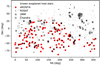 |
Fig. 1 X-ray detections of known exoplanet host stars in the sky. Known planet host stars are depicted as small grey dots. The Kepler field at RA = 300 deg as well as the increased density of known planets along the ecliptic due to the coverage by the K2 mission are visible. Detections in the German eROSITA sky with the eRASSl or eRASS2 survey are shown as filled red circles, previous detections with ROSAT, XMM-Newton, and Chandra are shown as filled black diamonds, open circles, and open squares, respectively. |
3.2 Flux conversions
The X-ray catalogues we used provide fluxes in slightly different energy bands. We opted for a commonly used soft X-ray band of 0.2–2 keV for the analysis of X-ray irradiation levels of exoplanets. We describe in the following how any necessary conversion factors were derived.
Similarly to the XMM-Newton catalogue, the intermediate eRASS catalogues use an assumed absorbed power-law spectral model to calculate X-ray fluxes from count rates. The assumed underlying model has an absorption column of NH = 1 x 10²⁰ and a power-law index of 1.7 for this intermediate version of the eRASS catalogues.
This is not a suitable spectral model for stellar coronae, which are described by an optically thin thermal plasma, with a contribution from absorption by the interstellar medium that tends to be small because detected exoplanets are typically located close to the Sun (more than 80% of the currently detected exoplanet host stars are located within a distance within 100 pc from the Sun).
In order to test whether an assumption of a typical coronal temperature of 0.3 keV is appropriate for the eROSITA-detected planet host stars, we first performed an analysis of X-ray hardness ratios in relation to coronal temperature. We simulated eROSITA spectra with Xspec version 12.11.1 (Arnaud 1996) using the eROSITA instrumental response files. Because the eRASS surveys are currently still shallow, we omitted an absorbing column and simulated spectra with a single temperature component for a range of coronal temperature parameters with kT between 0.1 and 1.0 keV steps, corresponding to temperatures of approximately 1.111 million K. We show some of these spectra in Fig. 4. For each of these simulated spectra, we calculated the model-based fluxes in the 0.2–0.6 (S), 0.6–2.3 (M) and 2.3–5.0 (H)keV energy bands, as well as their simulated count rates in these bands and the corresponding hardness ratios HR1 = (M – S)/(M + S)and HR2 = (H – M)/(H + M). We find that for the typical range of coronal temperature simulated by us, the hardness ratio HR2 is always very close to –1 because the effective area of eROSITA drops significantly beyond 2.3 keV. The simulated softer hardness ratio HR1 ranges from –0.9 to 0.8. We display the relation of the modelled coronal temperature and the simulated eROSITA hardness ratios in Fig. 5. This is valid for stars whose coronal spectra are dominated by a single temperature component. With multiple stars and strongly different coronal temperature components can behave differently with respect to their observed hardness ratios. In the observed data for our sample stars, the hardness ratio HR1 spans the full range between –1 and 1, with typical uncertainties of about ±0.2, that is, consistent with the simulated range of values. The majority of our observed stars is concentrated between values from –0.1 to 0.9 (Fig. 6), with a median of 0.34. This corresponds to a coronal temperature of about 0.3 keV. The observed values of HR2 agree with a value of –1 within observational uncertainties.
Given the observed hardness ratios, the eROSITA-detected sample agrees well with a typical coronal temperature of 0.3 keV, which we used to correct the final fluxes for a power-law to a stellar coronal model. We find the conversion factor between the fluxes to be Fx, coronal = 0.85Fx,poweriaw The eRASS stellar fluxes were calculated by applying the relative conversion factor to the power-law-derived fluxes from the intermediate eRASS catalogues.
For ROSAT, we again used a typical coronal temperature of kT = 0.3 keV to transform the fluxes from the 0.1 to 2.4 keV band into the canonical 0.2–2 keV band, using the WebPIMMS tool. The conversion factor is Fx,o.2-2kev = 0.87 x Fx,o.i-2.4kev.
For XMM-Newton, the 0.2–2 keV band already is one of the canonical bands given in the source catalogues, as the sum of bands 1 (0.2–0.5 keV), 2 (0.5–1.0 keV), and 3 (1.0–2.0 keV). However, because the XMM-Newton catalogue fluxes assume an underlying power-law spectrum with NH = 3 x 10²⁰ and a power-law index of 1.7 Rosen et al. (2016), we need to correct these fluxes to an underlying stellar coronal model. We again chose as a representative stellar model a coronal plasma with a temperature of 0.3 keV. XMM-Newton typically has deep pointings, detecting sources at larger distances than eROSITA, so that for this model a non-zero absorption column of NH = 3 x 10¹⁹ was used. The relative corrections compared to the power-law fluxes depend on the specific instruments and filters used in a given observations. Using the WebPIMMS tool6, we find a typical correction factor of Fx.coronai = 0.87Fx,poweriaw for the 0.2–2keV band for the combined signal from the EPIC cameras.
For Chandra, its second source catalogue also lists fluxes that are not explicitly model dependent, which are derived from the energies of the detected photons and the effective area of the instrument at these energies. We constructed the soft flux in the 0.2–2.0 keV band by combining the u (0.2–0.5 keV), s (0.5–1.2 keV), and m (1.2–2.0 keV) bands. However, it needs to be noted that depending on the instrument used in a given observation, the flux in the softest band may have gone undetected because the ACIS-I configuration has a very small effective area at the softest energies. Therefore some of the Chandra-derived fluxes may underestimate the true soft-band X-ray flux of a star.
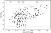 |
Fig. 2 X-ray to bolometric flux ratios of the exoplanet host stars in our sample vs their Gaia colour G – Rp; corresponding spectral types are given at the top of the figure. The horizontal dotted lines indicate the approximate upper and lower boundaries of typically observed flux ratios for main-sequence stars, with which our sample agrees well. |
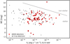 |
Fig. 3 Fluxes of the X-ray detected stars in our sample in the soft X-ray band and the WISE Wl infrared band, large red dots for eRASS detections, and small black dots for all X-ray detections. The statistical dividing line between objects of stellar and non-stellar nature (Salvato et al. 2018) is shown as the solid grey line. The only source that falls into the non-stellar part of the parameter space is an exoplanet-hosting cataclysmic variable. |
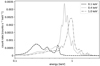 |
Fig. 4 Simulated stellar coronal spectra using the eROSITA instrumental response. A single-temperature coronal plasma model was used with temperatures of 0.1, 0.4, and 1 keV (1.1, 4.6, and 11.4million K). Almost all photons are emitted at energies below 2 keV even for very hot stellar coronae. |
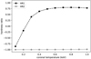 |
Fig. 5 Hardness ratios HR1 and HR2 from simulated stellar coronal eROSITA spectra as a function of coronal temperature. HR2 is always close to –1, rising only very slightly for very high temperatures, and HR1 rapidly rises from low to moderate coronal temperatures and then saturates at a value of about 0.75 for temperatures above 0.5 keV. |
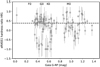 |
Fig. 6 Observed hardness ratio HR1 with 1σ uncertainties vs the Gaia G – RP colour for the stars in our sample. The median hardness ratio, corresponding to a coronal temperature of about 0.3 keV, is depicted by the dashed line. The quite blue star to the left is the Herbig Be star HD 100546, a known X-ray emitter (Skinner & Güdel 2020). |
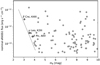 |
Fig. 7 Nominal X-ray fluxes from eRASSl vs. optical brightness for stars in our sample. For stars with an apparent Gaia magnitude brighter than 4mag, there is a clear trend towards high apparent eRASS fluxes, which can be attributed to optical loading. Some individual bright stars named in the plot can be expected to be only weak X-ray emitters because they are either lacking an outer convective envelope (ß Pic) or are coronal graveyard-type giants (Ayres et al. 2003). Furthermore, these specific stars are known to be X-ray dim from previous observations by other X-ray telescopes. |
3.3 Optical loading in eROSITA data
Objects with high optical brightness can cause spurious signals in X-ray observations. While X-ray CCDs are mainly sensitive to genuine X-ray photons, a large number of optical and infrared photons impinging on a CCD pixel within a readout time frame can release electrons in the CCD, which can be falsely attributed to an X-ray photon event; this is called ‘optical loading’.
We show the nominal X-ray fluxes from the eRASSl catalogue versus the optical Gaia magnitude of host stars in our sample in Fig. 7. We find that stars with an optical brightness of mG = 4 mag or brighter in the Gaia band display an apparent floor to their detected eRASS fluxes that rises with optical brightness. The A0V star ß Pic is one of these stars, and it is known to be X-ray dimmer by two orders of magnitude from previous pointed X-ray observations (Hempel et al. 2005; Günther et al. 2012). We therefore attribute the apparent X-ray flux of optically bright sources with mG ≲ 4 mag to optical loading in eROSITA observations and discard their contaminated eROSITA X-ray fluxes from the further analysis. We note that at least one optically bright star, ϵ Eridani, is a genuinely X-ray bright star that is known from observations with other X-ray telescopes (Poppenhaeger et al. 2010; Coffaro et al. 2020). However, a detailed spectral analysis of the eROSITA data to tease apart its coronal X-ray emission and the optical loading is beyond the scope of this work. We therefore use the measured ϵ Eri X-ray flux from XMM-Newton in the further analysis.
4 Results
4.1 New X-ray detections of exoplanet host stars
We show the positions of X-ray detected exoplanet host stars in the sky in Fig. 1. The total number of X-ray detected planet-hosting stars increases from 164 in the pre-eROSITA epoch to 241, that is, 77 are added through eRASSl and eRASS2. This increase can be expected to roughly double with the data from the Russian half of the eROSITA data. The X-ray detection fraction of exoplanet host stars in the German eROSITA sky is 89% within a distance of 5pc and 70% within 20 pc. At larger distances, the detection fraction drops rapidly (Fig. 8).
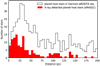 |
Fig. 8 Histogram of exoplanet host stars in distance bins of 5 pc (white with black outline) and the exoplanet host stars detected in the eRASSl survey (red) in the German eROSITA sky out to a distance of 200 pc. The detection fraction is high with about 70% out to 20 pc and then drops off rapidly. A small number of X-ray detections exists for planet host stars at larger distances. |
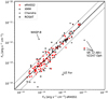 |
Fig. 9 Comparison of soft X-ray fluxes in the 0.2–2keV band for exoplanet host stars detected by more than one X-ray mission to fluxes detected by eRASSl. Stars detected by both eRASSl and eRASS2 are shown in red. Some individual outliers are marked by name; these objects are expected to display strong variability in X-rays. |
4.2 Flux comparisons for different X-ray missions
After performing the flux conversions for all data sets to cover the 0.2–2 keV range and correcting for an underlying stellar coronal model as laid out in Sect. 3.2, we compared the fluxes observed for stars that were detected in more than one mission. We show the X-ray fluxes for stars that were detected in eRASS 1 versus their fluxes observed in eRASS2, ROSAT, XMM-Newton, and Chandra in Fig. 9. About 75% of the observations display X-ray fluxes that agree within a corridor of 0.3 dex, which covers the typical low-level intrinsic variability of stellar coronae. The nominal flux discrepancies grow larger towards the faint end, which is to be expected because the flux uncertainties of the individual measurements increase as well. Additionally, when data sets from different surveys and/or pointed observations are compared, the shallowest survey will detect stars at the bottom of the survey sensitivity only when they happen to be temporarily X-ray bright, for example because of a flare. We see this effect in two directions here: the ROSAT survey is shallower than eRASS, which is why we see the ROSAT-eRASS data-points skewing towards higher ROSAT fluxes in the X-ray faint regime. On the other hand, eRASS tends to be much shallower than pointed XMM-Newton observations, which is why we see the XMM-eRASS data-points skewing towards higher eRASS fluxes at the X-ray dim end. For Chandra, there are not enough common detections to cause any visible skew.
Some individual notable outliers in the plot stem from intrinsically strongly variable stars, such as the binary T Tauri star V2247 Oph, the cataclysmic variable UZ For, and the M dwarf GJ 176, which is known to flare frequently (Loyd et al. 2018).
4.3 X-ray irradiation and mass loss of exoplanets
Exoplanets experiencing an intense high-energy irradiation are expected to lose parts of their atmosphere through a so-called energy-limited escape process, which is much more efficient than Jeans escape (Watson et al. 1981). The incoming XUV flux is assumed to be the driver of this process. The process describes that a certain part of the impinging high-energy flux heats the upper layers of the exoplanetary atmosphere, which expands upwards and can push the layers above out of the gravitational well of the exoplanet. There are known limitations to the energy-limited escape model, for example, it is expected for very high X-ray irradiation levels that hydrogen line cooling will start playing a more significant role, so that less energy is converted into atmospheric expansion (Murray-Clay et al. 2009). Magnetic effects such as stellar winds interacting with the planetary atmosphere or a planetary magnetosphere shielding the planet from winds may also play a role (Owen & Adams 2014; Cohen et al. 2015; Dong et al. 2017). In the context of this work, we use a simple energy-limited hydrodynamic escape model based on Lopez et al. (2012) and Owen & Jackson (2012), with an atmospheric mass-loss rate given by
 (1)
(1)
where ϵ is the efficiency of the atmospheric escape, which we assume to be 0.15, G is the gravitational constant, K is a factor representing the effect of Roche-lobe overflow, which we assume to be negligible for most systems and set to 1, Mpl is the mass of the planet, Rpl is the optical radius of the planet, FXUV is the XUV flux incident on the planet, and RXUV is the planetary radius at XUV wavelengths, which we assume to be 1.1 times the optical radius. For a detailed discussion of the assumptions made in this model, we refer to Poppenhaeger et al. (2021).
To estimate stellar XUV fluxes from X-ray fluxes alone, a variety of approaches exist (Sanz-Forcada et al. 2011; Linsky et al. 2014; Chadney et al. 2015; Johnstone et al. 2021; King & Wheatley 2021). We chose the conversion relation between X-ray and EUV fluxes by Sanz-Forcada et al. (2011), which uses spectral energy distributions determined for a sample of cool stars. We first converted our X-ray fluxes for the 0.2–2 keV band into the required input band of 0.1–2.4 keV for the conversion. This was derived using WebPIMMS, which yields a stellar coronal flux ratio of 1.15 between the 0.1–2.4 keV and the 0.2–2 keV flux for a typical coronal temperature of 0.3 keV. We then added the X-ray and EUV to obtain the XUV flux.
The resulting X-ray fluxes in the 0.2–2.0 keV band at the planetary orbits are shown in Fig. 10. The XUV fluxes are a factor of about five to ten higher than the X-ray fluxes alone. We immediately see the X-ray luminosity distribution of cool stars depicted in the vertical spread at any given planetary orbital semi-major axis. The planets that are amenable to follow-up observations of currently ongoing mass loss are planets that are transiting and are highly irradiated in the high-energy regime. We indicate the transiting planets by black circles and the new X-ray detections of host stars of transiting planets by additional black crosses. The clustering of transiting planets at close orbital distances comes from the geometric probability of a planet at a given inclination to be transiting, which strongly decreases for larger semi-major axes. Of the about 90 transiting planets with X-ray detected host stars, 26 stem from new eROSITA discoveries. Comparing the irradiation fluxes with the known evaporating exoplanets HD 189733 b and GJ 436 b (see the discussion in Sect. 5), we find that a total of 50 exoplanets in our sample show irradiation levels in excess of the one experienced by GJ 436 b, indicating that these exoplanets may be undergoing directly observable evaporation at the moment.
To determine the mass loss, data on both the planetary mass and radius are required. However, depending on the discovery method of a given planet, only the planetary mass or the radius may be known, but not necessarily both. In these cases, we used the mass-radius relationship by Chen & Kipping (2017) to estimate a planetary radius from the planet mass, or its mass from its radius. Chen & Kipping (2017) divided planets into a ‘terran’ regime with radii smaller than 2R⊕, in which masses are dominated by the rocky core, and a ‘Neptunian’ regime for planets with radii of 2R⊕ or more in which the gaseous envelope contains a significant fraction of the total mass. In our final mass-loss estimates we only included numeric estimates for exoplanets with radii larger than 1.6R⊕, based on Rogers (2015), who showed that exoplanets smaller than 1.6R⊕, are likely fully rocky and therefore unlikely to undergo any significant atmospheric mass loss.
We show the resulting mass-loss estimates in Fig. 11. A table of estimated mass-loss rates and the related X-ray quantities is available as an electronic data table (see the appendix). The highest mass-loss rates are as expected found for planets in very close orbits around their host stars. Here the vertical spread comes from both the X-ray luminosity distribution of the host stars and the spread in individual exoplanet masses and radii, which affects the estimated mass-loss rates as well. We find four new eROSITA measurements with expected mass-loss rates higher than for HD 189733 b, and 14 new eROSITA discoveries with expected mass-loss rates higher than for the Neptune GJ 436 b.
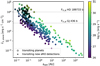 |
Fig. 10 X-ray irradiation fluxes of exoplanets vs their orbital semi-major axis. The vertical spread represents the intrinsic luminosity distribution of the host stars. Transiting exoplanets are marked with open black circles; new eROSITA X-ray detections among them are additionally marked with a black cross. For guidance, the X-ray irradiation fluxes of known evaporating exoplanets, the hot Jupiter HD 189733 b and the warm Neptune GJ 436 b, are shown as horizontal dotted lines. |
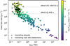 |
Fig. 11 Estimated mass-loss rates of exoplanets in the energy-limited escape model (see text for details). The vertical spread represents the intrinsic luminosity distribution of the host stars. Transiting exoplanets, which are in principle accessible to follow-up observations to detect ongoing mass loss, are marked with open black circles; new eROSITA X-ray detections among them are additionally marked with a black cross. For guidance, the estimated mass-loss rates of known evaporating exoplanets, the hot Jupiter HD 189733 b and the warm Neptune GJ 436 b, are shown as horizontal dotted lines. |
5 Discussion
5.1 Exoplanet mass-loss rates in context
While exoplanet evaporation rates can be estimated under the energy-limited mass-loss regime, there are also direct observations of ongoing evaporation for some planets. One possibility for direct mass-loss observations is through transit observations in the ultraviolet Ly-α line of hydrogen. The observed line shape is quite complex, even in the absence of exoplanetary mass loss. The host star produces emission in Ly-α, which is then partially absorbed by the interstellar medium, and finally, also Earth’s geocorona may add to the detected photons at the Ly-α wavelength. An actively evaporating exoplanetary atmosphere can be detected in the wings of the line, where planetary hydrogen moving at moderately high velocities causes additional absorption in the blue or red wing (or both) during the planetary transit. This was first successfully observed for the hot Jupiter HD 209458 b (Vidal-Madjar et al. 2003), and subsequent observations have targeted other hot Jupiters and even Neptunic planets. We focus here on the hot Jupiter HD 189733 b and the mini-Neptune GJ 436 b for our comparisons to the estimated mass-loss rates of other exoplanets.
HD 189733 b is a well-studied transiting hot Jupiter, orbiting a K0 star at a distance of about 20 pc from the Sun. The optical brightness of the host star makes this exoplanet one of the best-studied targets for transmission spectroscopy. Its absorption signature in the hydrogen Ly-α line showed that the planet is undergoing mass loss (Lecavelier Des Etangs et al. 2010). Because Ly-α observations can only quantify atomic (not ionised) hydrogen in the planetary atmosphere that is moving at relatively high speeds, determining mass-loss rates from these observations typically requires some additional model assumptions. Lecavelier Des Etangs et al. (2010) estimated the current mass-loss rate to be in the range of 109 and 1011 gs−1. Other estimates for the mass loss have been made, such as the model by Chadney et al. (2017), who calculated an upper limit to the mass-loss rate of HD 189733b of about 107 and 1012 g s−1 during stellar flares with large-scale proton events. Our calculation is based on the energy-limited escape model and estimates a current mass-loss rate of about 1.8 x 10¹¹ g s−1, which is at the upper end, but compatible with the estimates based on hydrogen Ly-α observations.
In contrast, GJ 436 b is a mini-Neptune in a close orbit around a nearby (9.75 pc) M dwarf that is only mildly X-ray active. This exoplanet has been observed to expel a spectacularly large hydrogen tail, as was first presented by Kulow et al. (2014) and then analysed in more detail by Ehrenreich et al. (2015). The atomic hydrogen tail observed in the Ly-α line covers almost half of the stellar disk during transits, with the egress being delayed by several hours compared to the broadband optical transit. This is consistent with an extended tail-like structure consisting of the evaporating atmosphere. While the hydrogen transit signal is strong and well observable, the modelled mass-loss rate is rather modest with about 4 x 10⁶ and 109gs−1 (Kulow et al. 2014). Simulations conducted by Villarreal D’Angelo et al. (2021) calculated a higher mass-loss rate of up to 1010gs−1. Our own results based on the high-energy irradiation estimate a current mass-loss rate of about 1.0 x 10⁹ gs−1, being bracketed by the hydrogen observations and simulations. This exoplanet shows that even more moderate mass-loss rates can produce strong observable signatures.
5.2 Interesting individual targets identified with eROSITA data
Transiting exoplanets with a high level of XUV irradiation are suitable for follow-up observations of ongoing mass loss, for example through transmission spectroscopy in the ultraviolet hydrogen Ly-α line or the metastable lines of helium (HeI 10830) in the infrared. We briefly discuss some particularly interesting systems here in terms of the planetary high-energy environment and mass loss.
TOI-251
TOI-251 is a solar-mass dwarf star with an apparent Gaia brightness of G = 9.8 mag, located at a distance of 99.5 pc from the Sun. It is a relatively young star with an age of 40–320 Myr, estimated from its rotation and magnetic activity (Zhou et al. 2021). TOI-251 hosts a mini-Neptune with a radius of 2.7R⊕ that orbits its host star in 4.9 days. We detect the host star with a high X-ray luminosity in the 0.2–2.0 keV band of LX = 1.5 x 1029 erg s−1 in eRASS1 and LX = 1.9 x 1029 erg s−1 in eRASS2. The source was previously detected in a pointed observation with ROSAT. The reported X-ray luminosity was slightly lower with LX = 1.1 x 1029 erg s−1 (Zhou et al. 2021). We derive that the orbiting mini-Neptune experiences an X-ray irradiation flux of about 16000 erg s−1 cm−2, corresponding to an estimated mass loss of about 3 x 10⁹ g s−1. This is higher than the estimated mass-loss rate of the known evaporating mini-Neptune GJ 436 b by a factor of 10, which makes this a highly interesting target for follow-up observations. Furthermore, this planet currently straddles the so-called evaporation gap in the radius distribution of planets (Fulton et al. 2017), indicating that it may currently undergo a marked change in radius due to evaporation. Poppenhaeger et al. (2021) recently showed for another young star-planet system, V1298 Tau and its four planets, that the early rotational evolution of the host star can make a significant difference in the initial-to-final radius relation of exoplanets. It is interesting in this context that TOI-251 seems to have already arrived on the slow/I-type sequence (Barnes 2010) of the stellar colour-rotation diagram (Zhou et al. 2021). This means that its future magnetic activity evolution and therefore the future planetary mass-loss evolution are relatively well predictable.
GJ 143
GJ 143 is a bright K dwarf located at a distance of 16.3 pc from the Sun, with an apparent Gaia brightness of G = 7.7 mag. It hosts two planets. Planet b is a Neptunic planet in an orbit of 35.6 days (Trifonov et al. 2019), and planet c is a small rocky planet in a closer orbit of 7.8 days (Dragomir et al. 2019). The host star is only moderately X-ray bright with a luminosity of LX = 1.7 x 1027 erg s−1 in the 0.2–2.0 keV band. However, this is enough to create a high-energy environment of roughly similar intensity as the one that is present for the evaporating Neptune GJ 436 b, which shows an X-ray irradiation flux of Fx,pi = 50erg s−1 cm−2. Planets b and c show irradiation fluxes of Fx,pl = 16 and 123 erg s−1 cm−2, respectively. While planet c is now rocky and likely does not have a thick gaseous envelope from which it can lose mass, it is possible that it was formed with a hydrogen-helium envelope that it lost over time, especially during higher X-ray activity epochs in the youth of the host star. We estimate that the larger planet b loses its atmosphere at a rate of about 5 x 10⁷ g s−1, that is, about an order of magnitude less than GJ 436 b. However, because the host star is optically brighter by a factor of about six, the ongoing evaporation of GJ 143 b may well be observable with current instrumentation.
K2-198 bcd
K2-198 is a K dwarf star that is located at a distance of 110.6 pc from the Sun, with an apparent Gaia brightness of G = 11.0 mag. It hast three known transiting planets (Mayo et al. 2018; Hedges et al. 2019): the innermost planet c orbits at a period of 3.4 days and has a radius of 1.4 R⊕ (Hedges et al. 2019), which places it in the regime of rocky planets. The middle planet d is a mini-Neptune with an orbital period of 7.5 days and a radius of 2.4 R⊕ (Hedges et al. 2019). The largest planet b is a Saturn-like planet in a wider orbit with an orbital period of 25.9 days and a radius of 4.2R⊕ (Mayo et al. 2018). The eROSITA data determined the host star X-ray luminosity to be 7.9 x 1028 erg s−1 in the 0.2–2.0 keV band. This places all three planets in an intense X-ray irradiation regime with fluxes at the planetary orbits of about FX, pl = 17 020, 5890, and 1950 erg s−1cm−2 for planets c, d, and b, respectively. The middle planet d is more strongly irradiated than the evaporating mini-Neptune GJ 436 b and can be expected to actively lose mass at a high estimated rate of 4 x 10¹⁰ g s−1. The innermost planet is likely to be rocky and might therefore no longer undergo any significantly mass loss. However, it is possible that it was formed with a primordial hydrogen-helium envelope that has been evaporated completely in the youth of the system. The highest-mass planet b shows an intermediate intensity of high-energy irradiation, which is lower than for the known evaporating hot Jupiter HD 189733 b, but higher than for GJ 436 b. We estimate it to undergo mass loss at a rate of 2 x 10¹⁰ gs−1.
K2-240 bc
K2-240 is an early-M dwarf that was discovered to host two transiting mini-Neptunes (Díez Alonso et al. 2018). It is located at a distance of 72.9 pc from the Sun and an apparent Gaia brightness of G = 12.6 mag. We determine its X-ray luminosity to be 3.7 x 1028 erg s−1 in the 0.2–2.0keV band. The two mini-Neptunes orbit the star in 6.0 and 20.5 days each. Their X-ray irradiation levels are well above those of the evaporating Neptune GJ 436b with FX,pl = 5020 and 980 ergs−1 cm−2 for planets b and c, respectively. We estimate their mass-loss rates to be Ṁ = 3 x 10¹⁰ and 5 x 10⁹ g s−1 for planets b and c. This is higher than for GJ 436 b by more than an order of magnitude for planet b. These two planets may be good targets for follow-up observations of ongoing evaporation.
6 Conclusion
We have presented a catalogue of X-ray luminosities of exo-planet host stars, high-energy irradiation levels of exoplanets, and their estimated atmospheric mass-loss rates. We combined new data from the eROSITA mission first and second all-sky surveys (eRASS1 and eRASS2) and amended our catalogue with archival data from ROSAT, XMM-Newton, and Chandra. We presented high-energy irradiation levels for 329 exoplanets, 108 of which stem from first-time detections with eROSITA, and mass-loss estimates for 287 exoplanets, 96 of which are derived from first-time eROSITA detections. Particularly interesting targets for follow-up observations of ongoing mass loss were found, including two multi-planet systems that can lead to unique insights into the evolution of exoplanetary atmospheres over time.
Acknowledgements
The authors thank Dr. Iris Traulsen for fruitful discussions of the XMM-Newton source catalogs, and Laura Ketzer for helpful input on the mass-radius relationship of exoplanets. This work is based on data from eROSITA, the primary instrument aboard SRG, a joint Russian-German science mission supported by the Russian Space Agency (Roskosmos), in the interests of the Russian Academy of Sciences represented by its Space Research Institute (IKI), and the Deutsches Zentrum für Luft- und Raumfahrt (DLR). The SRG spacecraft was built by Lavochkin Association (NPOL) and its subcontractors, and is operated by NPOL with support from the Max Planck Institute for Extraterrestrial Physics (MPE). The development and construction of the eROSITA X-ray instrument was led by MPE, with contributions from the Dr. Karl Remeis Observatory Bamberg & ECAP (FAU Erlangen-Nuernberg), the University of Hamburg Observatory, the Leibniz Institute for Astrophysics Potsdam (AIP), and the Institute for Astronomy and Astrophysics of the University of Tübingen, with the support of DLR and the Max Planck Society. The Argelander Institute for Astronomy of the University of Bonn and the Ludwig Maximilians Universität Munich also participated in the science preparation for eROSITA. The eROSITA data shown here were processed using the eSASS software system developed by the German eROSITA consortium. This work has made use of data from the Chandra X-ray Observatory, the ROSAT mission, and the XMM-Newton mission.
Appendix A X-ray fluxes of host stars with nearby stellar companions
Information about the flux corrections we applied for X-ray data from exoplanet host stars with nearby stellar companions is given below. We used information about stellar companions from Mugrauer (2019). We checked all host stars with a known stellar companion within 50″ for the X-ray instruments they were detected with, and considered a multi-star system to be likely blended in eROSITA, ROSAT, XMM-Newton, and Chandra if the stellar separation is below 8, 30, 8, and 1″, respectively. In these cases we divided the final listed X-ray flux, which we used for the calculations of the planetary irradiation and mass loss, by the number of blended stars (typically two). If a star is close to or below the blending separation, but X-ray data from a telescope with higher spatial resolution were available, we used the high-resolution data as the final listed flux.
18 Del
This star has a known stellar companion at a separation of about 29.2″, and the only available X-ray detection stems from ROSAT, which does not resolve the two stars. We therefore assigned 50% of the detected ROSAT flux at the position of this binary system to the exoplanet host star.
2MASS J01033563-5515561 A
This star has a known stellar companion at a separation of about 2″, and the existing XMMNewton and eRASS detections do not resolve the system. We therefore assigned 50% of the detected eRASS flux at the position of this binary system to the exoplanet host star.
CoRoT-2
This star has a known stellar companion at a separation of about 4.1″. The existing Chandra observations resolve the system, but the XMM-Newton observations does not. However, the Chandra data showed that the companion star is very X-ray faint and does not significantly contribute to the total X-ray flux of the system (Schröter et al. 2011), so that no adjustment was necessary.
DS Tuc A
This star has a known stellar companion at a separation of about 5″ (Newton et al. 2019). The current eRASS catalog does not resolve the two stars, and we therefore assigned 50% of the detected eRASS flux at the position of this binary system to the exoplanet host star.
GJ 338 B
This star has a known optically brighter stellar companion at a separation of 17″. The only existing X-ray detection stems from ROSAT, which does not resolve this wide binary. We therefore assigned 50% of the detected XMM-Newton flux at the position of this system to the exoplanet host star.
HAT-P-16
This is a hierarchical triple system, with a close stellar companion known at a separation of 0.4″ from the planet host star, and another wide companion at a separation of 23.3″. The close AB system is not resolved in the existing XMM-Newton detection, but the wider C component is not blended. We therefore assigned 50% of the detected XMM-Newton flux at the position of this system to the exoplanet host star.
HD 103774
This star has a known stellar companion at a separation of about 6.2″, and X-ray detections are present from eRASS1 and eRASS2, which do not resolve the two stars. We therefore assigned 50% of the detected eROSITA flux at the position of this binary system to the exoplanet host star.
HD 142
This star has a known stellar companion at a separation of about 3.9″, and X-ray detections are present from eRASS1 and eRASS2, which do not resolve the two stars. We therefore assigned 50% of the detected eROSITA flux at the position of this binary system to the exoplanet host star.
HD 162004
This star, also known as ψ 1 Dra B, has a known stellar companion at a separation of about 30″, and an X-ray detections is only present from ROSAT, which does not fully resolve the two stars. We therefore assigned 50% of the detected ROSAT flux at the position of this binary system to the exoplanet host star.
HD 189733
This star has a known stellar companion at a separation of about 11.4″. The ROSAT data do not resolve the system, but the Chandra and XMM-Newton observations do. Furthermore, it is known from an analysis of the Chandra data (Poppenhaeger et al. 2013) that the stellar companion is much less X-ray bright than the planet host star, therefore no adjustment was necessary.
HD 195019
This star has a known stellar companion at a separation of about 3.4″, and X-ray detections are present from eRASS2, which does not resolve the two stars. We therefore assigned 50% of the detected eROSITA flux at the position of this binary system to the exoplanet host star.
HD 19994
This is a triple system in which the planet host star is orbited by a close binary system (components B and C) at a separation of about 2.2″. X-ray detections are present from eRASS1 and eRASS2, which do not resolve the three stars. We therefore assigned one-third of the detected eROSITA flux at the position of this system to the exoplanet host star.
HD 212301
This star has a known stellar companion at a separation of about 4.4″, and an X-ray detection is present from eRASS1, which does not resolve the two stars. We therefore assigned 50% of the detected eROSITA flux at the position of this binary system to the exoplanet host star.
HD 65216
This is a triple system in which the planet host star is orbited by a close binary system (components B and C) at a separation of about 7.2″. X-ray detections are present from eRASS1 and eRASS2, which do not resolve the three stars. We therefore assigned one-third of the detected eROSITA flux at the position of this system to the exoplanet host star.
HIP 65 A
This star has a known stellar companion at a separation of about 4″, and the existing X-ray detections from eRASS do not resolve the stars. We therefore assigned 50% of the detected eROSITA flux at the position of this system to the exoplanet host star.
HR 858
HR 858 is a late-F type star that was reported to have a co-moving stellar companion of spectral type M at a separation of 8.4″ (Vanderburg et al. 2019). An X-ray source found in the eRASS datasets is located at the position of the secondary star and not the planet-hosting primary, therefore we attribute the detected X-ray flux to the secondary alone and do not report an X-ray detection for the planet host star based on the available data.
Kepler-1651
This star has a known stellar companion at a separation of about 4.1″, and an X-ray detection is present from ROSAT, which does not resolve the two stars. We therefore assigned 50% of the detected ROSAT flux at the position of this binary system to the exoplanet host star.
LTT 1445 A
This star has a known stellar companion at a separation of about 6.7″. The eRASS data detect flux from the position of the secondary alone, and we attribute the detected X-ray flux to the companion star alone.
τ Boo
This star has a close stellar companion at a separation of about 2″. X-ray detections exist with several X-ray missions, including Chandra. The existing Chandra observation is able to resolve the system and shows that the secondary is much fainter than the planet-hosting primary (Wood et al. 2018), so that no adjustment was necessary.
WASP-140
This star has a known stellar companion at a separation of about 7.2″, and an X-ray detection is present from eRASS2, which does not resolve the two stars. We therefore assigned 50% of the detected eROSITA flux at the position of this binary system to the exoplanet host star.
WASP-8
This star has a known stellar companion at a separation of about 4.5″, and an X-ray detection is present from eRASS1 and Chandra. Chandra observations have shown that the secondary is X-ray faint compared to the primary (Salz et al. 2015), and we therefore attribute the detected eRASS1 flux to the primary in our further calculations.
omi UMa
This star has a known stellar companion at a separation of about 6.8″, and an X-ray detection is present from ROSAT, which does not resolve the two stars. We therefore assigned 50% of the detected ROSAT flux at the position of this binary system to the exoplanet host star.
Appendix B Table of exoplanet irradiation fluxes and estimated mass-loss rates
We show an excerpt from the electronic data table with the most interesting columns for exoplanetary considerations in Table B.1. The full table is available at the CDS.
Excerpt from the available electronic data table.
References
- Andrae, R., Fouesneau, M., Creevey, O., et al. 2018, A&A, 616, A8 [NASA ADS] [CrossRef] [EDP Sciences] [Google Scholar]
- Arnaud, K. A. 1996, in ASP Conf. Ser., 101, Astronomical Data Analysis Software and Systems V, eds. G. H. Jacoby, & J. Barnes, 17 [NASA ADS] [Google Scholar]
- Ayres, T. R., Brown, A., & Harper, G. M. 2003, ApJ, 598, 610 [NASA ADS] [CrossRef] [Google Scholar]
- Baraffe, I., Chabrier, G., & Barman, T. 2010, Rep. Progr. Phys., 73, 016901 [CrossRef] [Google Scholar]
- Barnes, S. A. 2010, ApJ, 722, 222 [Google Scholar]
- Boller, T., Freyberg, M. J., Trümper, J., et al. 2016, A&A, 588, A103 [NASA ADS] [CrossRef] [EDP Sciences] [Google Scholar]
- Bours, M. C. P., Marsh, T. R., Breedt, E., et al. 2014, MNRAS, 445, 1924 [NASA ADS] [CrossRef] [Google Scholar]
- Brunner, H., Liu, T., Lamer, G., et al. 2022, A&A, 661, A1 (eROSITA EDR SI) [NASA ADS] [CrossRef] [EDP Sciences] [Google Scholar]
- Chadney, J. M., Galand, M., Unruh, Y. C., Koskinen, T. T., & Sanz-Forcada, J. 2015, Icarus, 250, 357 [Google Scholar]
- Chadney, J. M., Koskinen, T. T., Galand, M., Unruh, Y. C., & Sanz-Forcada, J. 2017, A&A, 608, A75 [NASA ADS] [CrossRef] [EDP Sciences] [Google Scholar]
- Chen, J., & Kipping, D. 2017, ApJ, 834, 17 [Google Scholar]
- Coffaro, M., Stelzer, B., Orlando, S., et al. 2020, A&A, 636, A49 [EDP Sciences] [Google Scholar]
- Cohen, O., Ma, Y., Drake, J. J., et al. 2015, ApJ, 806, 41 [NASA ADS] [CrossRef] [Google Scholar]
- Díez Alonso, E., González Hernández, J. I., Suárez Gómez, S. L., et al. 2018, MNRAS, 480, L1 [NASA ADS] [Google Scholar]
- Dong, C., Lingam, M., Ma, Y., & Cohen, O. 2017, ApJ, 837, L26 [NASA ADS] [CrossRef] [Google Scholar]
- Dragomir, D., Teske, J., Günther, M. N., et al. 2019, ApJ, 875, L7 [Google Scholar]
- Ehrenreich, D., Bourrier, V., Wheatley, P. J., et al. 2015, Nature, 522, 459 [Google Scholar]
- Evans, I. N., & Civano, F. 2018, Astron. Geophys., 59, 2.17 [NASA ADS] [CrossRef] [Google Scholar]
- Evans, I. N., Primini, F. A., Glotfelty, K. J., et al. 2010, ApJS, 189, 37 [NASA ADS] [CrossRef] [Google Scholar]
- Fortney, J. J., & Nettelmann, N. 2010, Space Sci. Rev., 152, 423 [CrossRef] [Google Scholar]
- France, K., Froning, C. S., Linsky, J. L., et al. 2013, ApJ, 763, 149 [Google Scholar]
- Fulton, B. J., Petigura, E. A., Howard, A. W., et al. 2017, AJ, 154, 109 [Google Scholar]
- Gaia Collaboration (Brown, A. G. A., et al.) 2018, A&A, 616, A1 [NASA ADS] [CrossRef] [EDP Sciences] [Google Scholar]
- Garmire, G. P., Bautz, M. W., Ford, P. G., Nousek, J. A., & Ricker, G. R. J., 2003, in Society of Photo-Optical Instrumentation Engineers (SPIE) Conference Series, 4851, X-Ray and Gamma-Ray Telescopes and Instruments for Astronomy, eds. J. E. Truemper, & H. D. Tananbaum, 28 [NASA ADS] [Google Scholar]
- Goździewski, K., Slowikowska, A., Dimitrov, D., et al. 2015, MNRAS, 448, 1118 [CrossRef] [Google Scholar]
- Güdel, M. 2004, A&ARv, 12, 71 [CrossRef] [Google Scholar]
- Günther, H. M., Wolk, S. J., Drake, J. J., et al. 2012, ApJ, 750, 78 [CrossRef] [Google Scholar]
- Hedges, C., Saunders, N., Barentsen, G., et al. 2019, ApJ, 880, L5 [NASA ADS] [CrossRef] [Google Scholar]
- Hempel, M., Robrade, J., Ness, J. U., & Schmitt, J. H. M. M. 2005, A&A, 440, 727 [NASA ADS] [CrossRef] [EDP Sciences] [Google Scholar]
- Jansen, F., Lumb, D., Altieri, B., et al. 2001, A&A, 365, L1 [NASA ADS] [CrossRef] [EDP Sciences] [Google Scholar]
- Johnstone, C. P., Bartel, M., & Güdel, M. 2021, A&A 649, A96 [EDP Sciences] [Google Scholar]
- King, G. W., & Wheatley, P. J. 2021, MNRAS, 501, L28 [Google Scholar]
- Kulow, J. R., France, K., Linsky, J., & Loyd, R. O. P. 2014, ApJ, 786, 132 [Google Scholar]
- Lecavelier Des Etangs, A., Ehrenreich, D., Vidal-Madjar, A., et al. 2010, A&A, 514, A72 [NASA ADS] [CrossRef] [EDP Sciences] [Google Scholar]
- Lindegren, L., Hernández, J., Bombrun, A., et al. 2018, A&A, 616, A2 [NASA ADS] [CrossRef] [EDP Sciences] [Google Scholar]
- Linsky, J. L., Fontenla, J., & France, K. 2014, ApJ, 780, 61 [Google Scholar]
- Lopez, E. D., Fortney, J. J., & Miller, N. 2012, ApJ, 761, 59 [Google Scholar]
- Loyd, R. O. P., France, K., Youngblood, A., et al. 2018, ApJ, 867, 71 [Google Scholar]
- Mayo, A. W., Vanderburg, A., Latham, D. W., et al. 2018, AJ, 155, 136 [Google Scholar]
- Mayor, M., & Queloz, D. 1995, Nature, 378, 355 [Google Scholar]
- Merloni, A., Predehl, P., Becker, W., et al. 2012, ArXiv e-prints, [arXiv:1289.3114] [Google Scholar]
- Monsch, K., Ercolano, B., Picogna, G., Preibisch, T., & Rau, M. M. 2019, MNRAS, 483, 3448 [Google Scholar]
- Mugrauer, M. 2019, MNRAS, 490, 5088 [Google Scholar]
- Murray, S. S., Chappell, J. H., Kenter, A. T., et al. 1997, in Society of Photo-Optical Instrumentation Engineers (SPIE) Conference Series, 3114, EUV, X-Ray, and Gamma-Ray Instrumentation for Astronomy VIII, eds. O. H. Siegmund, & M. A. Gummin, 11 [NASA ADS] [Google Scholar]
- Murray-Clay, R. A., Chiang, E. I., & Murray, N. 2009, ApJ, 693, 23 [Google Scholar]
- Newton, E. R., Mann, A. W., Tofflemire, B. M., et al. 2019, ApJ, 880, L17 [Google Scholar]
- Nortmann, L., Pallé, E., Salz, M., et al. 2018, Science, 362, 1388 [Google Scholar]
- Owen, J. E., & Adams, F. C. 2014, MNRAS, 444, 3761 [Google Scholar]
- Owen, J. E., & Jackson, A. P. 2012, MNRAS, 425, 2931 [Google Scholar]
- Poppenhaeger, K., & Wolk, S. J. 2014, A&A, 565, L1 [NASA ADS] [CrossRef] [EDP Sciences] [Google Scholar]
- Poppenhaeger, K., Robrade, J., & Schmitt, J. H. M. M. 2010, A&A, 515, A98 [NASA ADS] [CrossRef] [EDP Sciences] [Google Scholar]
- Poppenhaeger, K., Schmitt, J. H. M. M., & Wolk, S. J. 2013, ApJ, 773, 62 [Google Scholar]
- Poppenhaeger, K., Ketzer, L., & Mallonn, M. 2021, MNRAS, 500, 4560 [Google Scholar]
- Predehl, P., Andritschke, R., Arefiev, V., et al. 2021, A&A, 647, A1 [EDP Sciences] [Google Scholar]
- Raghavan, D., McAlister, H. A., Henry, T. J., et al. 2010, ApJS, 190, 1 [Google Scholar]
- Rogers, L. A. 2015, ApJ, 801, 41 [Google Scholar]
- Rosen, S. R., Webb, N. A., Watson, M. G., et al. 2016, A&A, 590, A1 [NASA ADS] [CrossRef] [EDP Sciences] [Google Scholar]
- Salvato, M., Buchner, J., Budavári, T., et al. 2018, MNRAS, 473, 4937 [Google Scholar]
- Salz, M., Schneider, P. C., Czesla, S., & Schmitt, J. H. M. M. 2015, A&A, 576, A42 [NASA ADS] [CrossRef] [EDP Sciences] [Google Scholar]
- Salz, M., Schneider, P. C., Fossati, L., et al. 2019, A&A, 623, A57 [NASA ADS] [CrossRef] [EDP Sciences] [Google Scholar]
- Sanz-Forcada, J., Micela, G., Ribas, I., et al. 2011, A&A, 532, A6 [NASA ADS] [CrossRef] [EDP Sciences] [Google Scholar]
- Saxton, R. D., Read, A. M., Esquej, P., et al. 2008, A&A, 480, 611 [NASA ADS] [CrossRef] [EDP Sciences] [Google Scholar]
- Schmitt, J. H. M. M., Fleming, T. A., & Giampapa, M. S. 1995, ApJ, 450, 392 [Google Scholar]
- Schröter, S., Czesla, S., Wolter, U., et al. 2011, A&A, 532, A3 [NASA ADS] [CrossRef] [EDP Sciences] [Google Scholar]
- Schwope, A. D., & Thinius, B. D. 2014, Astron. Nachr., 335, 357 [Google Scholar]
- Skinner, S. L., & Güdel, M. 2020, ApJ, 888, 15 [NASA ADS] [CrossRef] [Google Scholar]
- Spake, J. J., Sing, D. K., Evans, T. M., et al. 2018, Nature, 557, 68 [Google Scholar]
- Strüder, L., Briel, U., Dennerl, K., et al. 2001, A&A, 365, L18 [Google Scholar]
- Sunyaev, R., Arefiev, V., Babyshkin, V., et al. 2021, A&A, 656, A132 [NASA ADS] [CrossRef] [EDP Sciences] [Google Scholar]
- Traulsen, I., Schwope, A. D., Lamer, G., et al. 2020, A&A, 641, A137 [NASA ADS] [CrossRef] [EDP Sciences] [Google Scholar]
- Trifonov, T., Rybizki, J., & Kürster, M. 2019, A&A, 622, L7 [NASA ADS] [CrossRef] [EDP Sciences] [Google Scholar]
- Truemper, J. 1982, Adv. Space Res., 2, 241 [Google Scholar]
- Turner, M. J. L., Abbey, A., Arnaud, M., et al. 2001, A&A, 365, L27 [CrossRef] [EDP Sciences] [Google Scholar]
- Vanderburg, A., Huang, C. X., Rodriguez, J. E., et al. 2019, ApJ, 881, A19 [Google Scholar]
- Vidal-Madjar, A., Lecavelier des Etangs, A., Désert, J. M., et al. 2003, Nature, 422, 143 [Google Scholar]
- Villarreal D’Angelo, C., Vidotto, A. A., Esquivel, A., Hazra, G., & Youngblood, A. 2021, MNRAS, 501, 4383 [CrossRef] [Google Scholar]
- Voges, W., Aschenbach, B., Boller, T., et al. 1999, A&A, 349, 389 [NASA ADS] [Google Scholar]
- Voges, W., Aschenbach, B., Boller, T., et al. 2000, IAU Circ., 7432, 3 [NASA ADS] [Google Scholar]
- Watson, A. J., Donahue, T. M., & Walker, J. C. G. 1981, Icarus, 48, 150 [NASA ADS] [CrossRef] [Google Scholar]
- Watson, M. G., Schröder, A. C., Fyfe, D., et al. 2009, A&A, 493, 339 [NASA ADS] [CrossRef] [EDP Sciences] [Google Scholar]
- Weisskopf, M. C., Brinkman, B., Canizares, C., et al. 2002, PASP, 114, 1 [NASA ADS] [CrossRef] [Google Scholar]
- Wood, B. E., Laming, J. M., Warren, H. P., & Poppenhaeger, K. 2018, ApJ, 862, 66 [Google Scholar]
- Yelle, R. V. 2004, Icarus, 170, 167 [NASA ADS] [CrossRef] [Google Scholar]
- Zhou, G., Quinn, S. N., Irwin, J., et al. 2021, AJ, 161, 2 [Google Scholar]
In cases where the observed co-added epochs in the catalogues spanned more than three years and proper motions were large or not available, the maximum allowed matching radius was doubled.
All Tables
All Figures
|
Fig. 1 X-ray detections of known exoplanet host stars in the sky. Known planet host stars are depicted as small grey dots. The Kepler field at RA = 300 deg as well as the increased density of known planets along the ecliptic due to the coverage by the K2 mission are visible. Detections in the German eROSITA sky with the eRASSl or eRASS2 survey are shown as filled red circles, previous detections with ROSAT, XMM-Newton, and Chandra are shown as filled black diamonds, open circles, and open squares, respectively. |
| In the text | |
|
Fig. 2 X-ray to bolometric flux ratios of the exoplanet host stars in our sample vs their Gaia colour G – Rp; corresponding spectral types are given at the top of the figure. The horizontal dotted lines indicate the approximate upper and lower boundaries of typically observed flux ratios for main-sequence stars, with which our sample agrees well. |
| In the text | |
|
Fig. 3 Fluxes of the X-ray detected stars in our sample in the soft X-ray band and the WISE Wl infrared band, large red dots for eRASS detections, and small black dots for all X-ray detections. The statistical dividing line between objects of stellar and non-stellar nature (Salvato et al. 2018) is shown as the solid grey line. The only source that falls into the non-stellar part of the parameter space is an exoplanet-hosting cataclysmic variable. |
| In the text | |
|
Fig. 4 Simulated stellar coronal spectra using the eROSITA instrumental response. A single-temperature coronal plasma model was used with temperatures of 0.1, 0.4, and 1 keV (1.1, 4.6, and 11.4million K). Almost all photons are emitted at energies below 2 keV even for very hot stellar coronae. |
| In the text | |
|
Fig. 5 Hardness ratios HR1 and HR2 from simulated stellar coronal eROSITA spectra as a function of coronal temperature. HR2 is always close to –1, rising only very slightly for very high temperatures, and HR1 rapidly rises from low to moderate coronal temperatures and then saturates at a value of about 0.75 for temperatures above 0.5 keV. |
| In the text | |
|
Fig. 6 Observed hardness ratio HR1 with 1σ uncertainties vs the Gaia G – RP colour for the stars in our sample. The median hardness ratio, corresponding to a coronal temperature of about 0.3 keV, is depicted by the dashed line. The quite blue star to the left is the Herbig Be star HD 100546, a known X-ray emitter (Skinner & Güdel 2020). |
| In the text | |
|
Fig. 7 Nominal X-ray fluxes from eRASSl vs. optical brightness for stars in our sample. For stars with an apparent Gaia magnitude brighter than 4mag, there is a clear trend towards high apparent eRASS fluxes, which can be attributed to optical loading. Some individual bright stars named in the plot can be expected to be only weak X-ray emitters because they are either lacking an outer convective envelope (ß Pic) or are coronal graveyard-type giants (Ayres et al. 2003). Furthermore, these specific stars are known to be X-ray dim from previous observations by other X-ray telescopes. |
| In the text | |
|
Fig. 8 Histogram of exoplanet host stars in distance bins of 5 pc (white with black outline) and the exoplanet host stars detected in the eRASSl survey (red) in the German eROSITA sky out to a distance of 200 pc. The detection fraction is high with about 70% out to 20 pc and then drops off rapidly. A small number of X-ray detections exists for planet host stars at larger distances. |
| In the text | |
|
Fig. 9 Comparison of soft X-ray fluxes in the 0.2–2keV band for exoplanet host stars detected by more than one X-ray mission to fluxes detected by eRASSl. Stars detected by both eRASSl and eRASS2 are shown in red. Some individual outliers are marked by name; these objects are expected to display strong variability in X-rays. |
| In the text | |
|
Fig. 10 X-ray irradiation fluxes of exoplanets vs their orbital semi-major axis. The vertical spread represents the intrinsic luminosity distribution of the host stars. Transiting exoplanets are marked with open black circles; new eROSITA X-ray detections among them are additionally marked with a black cross. For guidance, the X-ray irradiation fluxes of known evaporating exoplanets, the hot Jupiter HD 189733 b and the warm Neptune GJ 436 b, are shown as horizontal dotted lines. |
| In the text | |
|
Fig. 11 Estimated mass-loss rates of exoplanets in the energy-limited escape model (see text for details). The vertical spread represents the intrinsic luminosity distribution of the host stars. Transiting exoplanets, which are in principle accessible to follow-up observations to detect ongoing mass loss, are marked with open black circles; new eROSITA X-ray detections among them are additionally marked with a black cross. For guidance, the estimated mass-loss rates of known evaporating exoplanets, the hot Jupiter HD 189733 b and the warm Neptune GJ 436 b, are shown as horizontal dotted lines. |
| In the text | |
Current usage metrics show cumulative count of Article Views (full-text article views including HTML views, PDF and ePub downloads, according to the available data) and Abstracts Views on Vision4Press platform.
Data correspond to usage on the plateform after 2015. The current usage metrics is available 48-96 hours after online publication and is updated daily on week days.
Initial download of the metrics may take a while.