| Issue |
A&A
Volume 694, February 2025
|
|
|---|---|---|
| Article Number | A179 | |
| Number of page(s) | 14 | |
| Section | Stellar structure and evolution | |
| DOI | https://doi.org/10.1051/0004-6361/202452580 | |
| Published online | 12 February 2025 | |
Planetary inward migration as the potential cause of GJ 504’s fast rotation and bright X-ray luminosity
New constraints from eROSITA
1
STAR Institute, Université de Liège, Liège, Belgium
2
Istituto Nazionale di Astrofisica – Osservatorio Astronomico di Roma, Via Frascati 33, I-00040 Monteporzio Catone, Italy
3
Institut für Astronomie und Astrophysik, Eberhard-Karls Universität Tübingen, Sand 1, 72076 Tübingen, Germany
4
Leiden Observatory, Leiden University, PO Box 9513 2300 RA Leiden, The Netherlands
5
Institut de Recherche en Astrophysique et Planétologie, Université de Toulouse, CNRS, IRAP/UMR 5277, 14 Avenue Edouard Belin, F-31400 Toulouse, France
6
Leibniz Institute for Astrophysics Potsdam (AIP), An der Sternwarte 16, 14482 Potsdam, Germany
7
Institute for Physics and Astronomy, University of Potsdam, Karl-Liebknecht-Str. 24/25, 14476 Potsdam-Golm, Germany
⋆ Corresponding author; camilla.pezzotti@uliege.be
Received:
11
October
2024
Accepted:
30
December
2024
Context. The discovery of an increasing variety of exoplanets in very close orbits around their host stars raised many questions about how stars and planets interact and to what extent host stars’ properties may be influenced by the presence of close-by companions. Understanding how the evolution of stars is impacted by the interactions with their planets is indeed fundamental to disentangling their intrinsic evolution from star-planet-interaction (SPI) induced phenomena. In this context, GJ 504 is a promising candidate for a star that underwent strong SPI. Its unusually short rotational period (Prot ∼ 3.4 days), while being in contrast with what is expected of single-star models, could result from the inward migration of a close-by, massive companion (Mpl ≥ 2 MJ), pushed towards its host by the action of tides. Moreover, its brighter emission in the X-ray luminosity may hint at a rejuvenation of the dynamo process sustaining the stellar magnetic field, which is a consequence of the SPI-induced spin-up.
Aims. We aim to study the evolution of GJ 504 and establish whether by invoking the engulfment of a planetary companion we can better reproduce its rotational period and X-ray luminosity.
Methods. We simulated the past evolution of the star by assuming two different scenarios: ‘star without close-by planet’ and ‘star with close-by planet’. In the second scenario, we use our SPI code to investigate how the inward migration and eventual engulfment of a giant planet driven by stellar tides may spin-up the stellar surface and rejuvenate its dynamo. We compare our theoretical tracks with archival-rotational-period and X-ray data of GJ 504 collected from the all-sky surveys of the ROentgen Survey with an Imaging Telescope Array (eROSITA) on board the Russian Spektrum-Roentgen-Gamma mission (SRG).
Results. Despite the large uncertainty on the stellar age, we find that the second evolutionary scenario characterised by the inward migration of a massive planetary companion is in better agreement with the short rotational period and the bright X-ray luminosity of GJ 504; thus, it strongly favours the inward migration scenario over the one in which close-by planets have no tidal impact on the star.
Key words: planets and satellites: dynamical evolution and stability / planet-star interactions / stars: activity / stars: evolution / planetary systems / stars: rotation
© The Authors 2025
 Open Access article, published by EDP Sciences, under the terms of the Creative Commons Attribution License (https://creativecommons.org/licenses/by/4.0), which permits unrestricted use, distribution, and reproduction in any medium, provided the original work is properly cited.
This article is published in open access under the Subscribe to Open model. Subscribe to A&A to support open access publication.
1. Introduction
With the discovery of thousands of exoplanets in the last few decades (5678 as of June 2024; Nasa Exoplanet Archive1), the need to precisely characterise their host stars has become crucial in order to accurately derive the properties of the systems (e.g. Adibekyan et al. 2018) and understand their formation and evolution. From their birth, stars shape the evolution of exoplanetary systems. At the same time, host stars’ properties may be significantly influenced by the presence of interacting close-by planetary companions, potentially resulting in anomalous rotational periods (e.g. Privitera et al. 2016; Ilić et al. 2024) and magnetic activity, with brighter X-ray luminosity emissions (e.g. Shkolnik et al. 2003; Poppenhaeger & Wolk 2014; Pillitteri et al. 2022; Ilić et al. 2023) (among others). Understanding how the evolution of stars is impacted by the interactions with their planets is thus fundamental to disentangling their intrinsic evolution from SPI-induced phenomena on the one hand and to helping determine properties that could not be derived otherwise (e.g. tracing back their rotational history) on the other.
In this context, GJ 504 (a.k.a. HD 115383, TIC 397587084) is a promising candidate for a star that underwent strong star-planet interactions. GJ 504 is an isolated G0 spectral type star that is slightly more massive than the Sun (M⋆ ∼ 1.22 M⊙) and hosts a directly imaged substellar companion at a projected distance of ∼43.5 AU (Kuzuhara et al. 2013). Because of the significant uncertainties in determining GJ 504’s evolutionary state, with age estimations varying from hundreds of megayears to several gigayears (Valenti & Fischer 2005; Takeda et al. 2007; Holmberg et al. 2009; da Silva et al. 2012; Kuzuhara et al. 2013; Fuhrmann & Chini 2015; D’Orazi et al. 2017; Di Mauro et al. 2022), the nature of the companion is still hotly debated, and very different values for its mass have been proposed in the literature (1 ≲ Mc/MJ ≲ 25) (Kuzuhara et al. 2013; Fuhrmann & Chini 2015).
Establishing the age of isolated stellar objects is particularly hard. Different methods could be used (Soderblom et al. 2014), including gyrochronology and activity indicators, for the age-rotation-activity relation (Skumanich 1972; Barnes 2007) or comparison of classical spectroscopic parameters with model isochrones (e.g. Pont & Eyer 2004). Kuzuhara et al. (2013) estimated the age of GJ 504 via several methods, but they considered the one derived from gyrochronology and activity indicators, based on Prot = 3.329 days (Donahue et al. 1996; Messina et al. 2003) and chromospheric activity indices (Ca II H and K lines, log(RHK′) = −4.45), as the most likely one, giving the value 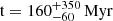 . A few years later, Fuhrmann & Chini (2015) carried out a detailed analysis of high-resolution, high-quality spectra, which led to a major revision of the stellar gravity parameter log(g) = 4.23 ± 0.10, which is about 8% smaller than the value in Kuzuhara et al. (2013). From the isochrone-fitting method, they found an age much closer to the one of the Sun (
 ) (Fuhrmann & Chini 2015). To explain the short rotational period, intense chromospheric activity, and bright X-ray luminosity (Log(LX/LBol) = − 4.42, Voges et al. 1999; Wright et al. 2011) and to reconcile these indicators with the isochronal age, Fuhrmann & Chini (2015) invoked the engulfment2 of a close-by planetary companion that would have spun up the stellar surface and enhanced its activity levels (Oetjens et al. 2020). D’Orazi et al. (2017) reassessed the fundamental properties of GJ 504, finding that a comparison of their spectroscopic parameters with isochrones provided an age between 1.8 and 3.5 Gyr, with a most probable value of t ≈ 2.5 Gyr. They also envisaged a possible engulfment scenario to reconcile the different age indicators and tested this hypothesis by means of a tidal-evolution code. They found that the engulfment of a hot Jupiter, with an initial mass no larger than ≈3 MJ and initial orbital distance of ≈0.03 AU, could be a very likely scenario. Bonnefoy et al. (2018) revisited the system by means of high-contrast imaging and interferometric and radial-velocity observations. From their analysis, they retrieved an interferometric radius for the host star of R = (1.35 ± 0.04) R⊙, which is compatible with two isochronal ages: (21 ± 2) Myr and (4.0 ± 1.8) Gyr. The mass of the substellar companion would correspond to
  or
or  , respectively. The authors also revised the almost pole-on line-of-sight stellar-rotation-axis inclination, which is
  degrees or
  degrees. They also excluded the presence of additional objects (with 90% probability) more massive than 2.5 and 30 MJ with semi-major axes in the range of 0.01 − 80 AU for the young and old isochronal ages, respectively. More recently, Di Mauro et al. (2022) attempted to employ asteroseismic techniques on the observational data collected by the Transiting Exoplanet Survey Satellite space mission (TESS, Ricker et al. 2014) to accurately characterise GJ 504. Unfortunately, the non-detection of solar-like oscillations, which Di Mauro et al. (2022) ascribed to the high level of the stellar magnetic activity, hindered their analysis. Nevertheless, the results deduced by TESS photometric data – supported by the Mount Wilson Observatory long-term campaign spanning nearly 30 years – and modelling procedures allowed the authors to refine the fundamental parameters of GJ 504. Among these, they derived an age ≤2.6 Gyr, which is in agreement with previous findings by Kuzuhara et al. (2013) and D’Orazi et al. (2017) within the quoted uncertainties. From the TESS light curves, they also identified a clear modulation corresponding to a rotational period of Prot = 3.4 days, which confirms the average value used in Kuzuhara et al. (2013). Finally, from Mount Wilson Observatory data they obtained the detection of a main magnetic cycle of 11.97 years, which, together with the relatively short rotational period, located GJ 504 before the transition to the weakened magnetic braking regime, as theorised by van Saders et al. (2016). During this transition the large-scale magnetic field would fail to efficiently brake the stellar surface.
The aim of our work is to study the peculiar properties of GJ 504 by testing the impact of a putative, close-by planet’s inward migration on the evolution of the stellar rotational period and X-ray luminosity. For this reason, we first looked for the optimal stellar parameters representative of GJ 504 by means of a minimisation procedure based on classical spectroscopic and interferometric parameters and correspondingly computed best-fit stellar models (see Sect. 2.1). Subsequently, we coupled the stellar models to our SPI code (see Sect. 2.2), in which the evolution of the stellar surface-rotation rate and X-ray luminosity is computed simultaneously to the evolution of the orbit of a close-by planetary companion; this is driven by the dissipation of tides within the host star (see Sect. 4). We envisage two evolutionary scenarios:
-
The star-without-close-by-planet scenario (Sect. 4.1), in which no massive or close-by companions affect the evolution of the host star
-
The star-with-close-by-planet scenario (Sect. 4.2), in which a putative, close-by planet strongly impacts the evolution of its host star3
We thus compare the results of the simulations with observational data for the rotational period and X-ray luminosity. For the latter one, in addition to the ROSAT (Truemper 1982) data, we give a detailed analysis of the X-ray data taken with the ROentgen Survey with an Imaging Telescope Array (eROSITA; Predehl et al. 2021) on board the Russian Spektrum-Roentgen-Gamma mission (SRG; Sunyaev et al. 2021) (see Sect. 3) and compare it with previous results found in Foster et al. (2022). We searched for an X-ray counterpart of GJ 504 among the sources listed in the five all-sky surveys of eROSITA (eRASS; Merloni et al. 2024). The first four surveys are completed and count six months of observation, while the last survey was suspended after almost two months because the science operations of the instrument were paused. Finally, in Sect. 5 we draw our conclusions.
2. Method and physics
To carry out our study on GJ 504, we proceeded according to the following steps. Firstly, we derived the optimal parameters for the star (initial mass, radius, chemical composition, etc.) by means of a minimisation technique based on classical spectroscopic and interferometric parameters (unfortunately asteroseismic indicators are not available for this star); secondly, best-fit stellar models were computed based on the optimal parameters found before; finally, the stellar models are coupled to our SPI code in which the evolution of the star is computed by envisaging two potential scenarios. These are the star-without-close-by-planet and the star-with-close-by-planet scenarios.
2.1. Optimal parameter search and stellar model
To compute stellar models for GJ 504, we started by deriving optimal stellar parameters by means of a two-step, global, and local-minimisation procedure. For the global minimisation, we employed the SPInS software (Lebreton & Reese 2020), which is based on a Markov chain Monte Carlo (MCMC) approach and Bayesian statistics, to derive probability distribution functions for stellar parameters. For the local minimisation, we used the Levenberg-Marquardt algorithm (e.g. Miglio & Montalbán 2005; Farnir et al. 2020).
In both minimisation procedures, we used models computed with the Liège stellar evolution code (CLES) (e.g. Scuflaire et al. 2008). For the setup of input physics, we considered the FreeEOS (Irwin 2012) equation of state, AGSS09 (Asplund et al. 2009) abundances, and OPAL (Iglesias & Rogers 1996) opacity tables for solar mixture. The classical mixing-length theory was applied for convection, with a solar calibrated value αMLT = 2.01. For the outer boundary conditions, we used Vernazza et al. (1981).
In this context, we aimed to determine the values of four free parameters (M⋆, age, X0, and Z0) using four observational constraints taken from Di Mauro et al. (2022) (see references therein): Teff = (6205 ± 20) K, R = (1.35 ± 0.04) R⊙, [Fe/H] = 0.22 ± 0.04, and log(g) = 4.29 ± 0.07.
The results obtained from the first step of modelling with SPInS are M⋆ = (1.30 ± 0.05) M⊙, X0 = 0.70 ± 0.02, Z0 = 0.025 ± 0.002, and age =(1.81 ± 0.46) Gyr. While this solution is limited to the fixed input physics used for the computation of the model grid, in the second step the local minimisation procedure allows us to further explore the parameter space thanks to the use of the Levenberg-Marquardt algorithm. With the computation of models on the fly, it is possible to investigate the impact of changing the input physics on the stellar parameters. In particular, we tested the effect of including a moderate amount of overshooting (αOv = 0.1 Hp, with Hp being the pressure scale height). We also changed the outer boundary conditions, using the Eddington T(τ) relations, and the corresponding solar calibrated value for the mixing length αMLT = 1.8. The optimal parameters derived by means of this procedure are M⋆ = (1.29 ± 0.21) M⊙, X0 = 0.70 ± 0.09, Z0 = 0.025 ± 0.002, and age =(2.11 ± 1.75) Gyr.
Both solutions agree very closely on the mean values, but from the local minimisation procedure we derived larger uncertainties, especially for the age. This is due not only to the broader input physics used in the Levenberg-Marquardt algorithm, but also to the intrinsic differences in comparison to SPInS for the computation of the uncertainties.
In general, these solutions appear to be in good agreement with the ones found in Di Mauro et al. (2022), although a smaller uncertainty on the age estimation was found in our case. According to our analysis, an age as young as ≈200 Myr seems to be disfavoured for this star. Nevertheless, it is worth stressing that only seismic constraints would likely allow us to derive more precise age estimates (Soderblom 2010).
We thus proceeded by computing the evolutionary sequence of GJ 504 using CLES, for which the derived optimal parameters (M⋆ = 1.29 M⊙, X0 = 0.70, Z0 = 0.025) were provided as input and constraints. According to this model, GJ 504 is a main-sequence (MS) star, with a central abundance of hydrogen of Xc = 0.37, mass of the convective envelope of Menv = 2.5 × 10⁻³ M⋆, radius of the convective envelope of Renv = 0.18 R⋆, and an inner convective core with Mcc = 1.3 × 10⁻² M⋆ and Mcc = 4.3 × 10⁻² R⋆. In Fig. 1, we show the evolutionary track corresponding to the best-fit model. For a detailed description of the physics included in CLES, we refer the interested reader to Scuflaire et al. (2008).
 |
Fig. 1. Hertzsprung-Russell diagram of GJ 504 as obtained from best-fit stellar model (Teff = 6202 K, log(g) = 4.29, R = 1.35 R⊙, L/L⊙ = 2.43) computed with CLES. |
As mentioned above, the computed evolutionary sequence of GJ 504 is provided to our SPI code to study its past evolution. Given the significant uncertainties derived on GJ 504’s parameters, in the following we discuss our results considering the broadest age interval ((0.36 − 3.86) Gyr) and show both average values and their corresponding uncertainties in the figures for comparison. While different age values would correspond to different stellar masses and chemical compositions, considering the physics included in our SPI code we can reasonably assume that our conclusion remains valid within the 4D space (M⋆, age, X0, and Z0) of variation for our best-fit stellar model.
2.2. Star-planet-interaction code
The stellar models computed for GJ 504 are provided as input to our SPI code. In this code it is possible to compute the rotational evolution of the star while accounting for two main types of star-planet interaction: gravitational-tidal and radiative (e.g. Cuntz et al. 2000; Vidotto 2020; Strugarek 2024). While a more detailed description of the physics implemented in the code is provided in Privitera et al. (2016), Rao et al. (2018), Pezzotti et al. (2021), Fellay et al. (2023), in the following we just recall the equations of interest for the evolution of a putative planet orbiting closely around GJ 504.
2.2.1. Host-star surface-rotation evolution
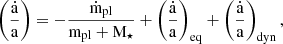
The evolution of the stellar surface-rotation rate is computed assuming that the host-star rotates as a solid body on the pre-main-sequence (PMS) and MS phases (Rao et al. 2021). Given the relative shallowness of the convective envelope characterising GJ 504 and the fact that the differential rotation in this region is less significant compared to the almost flat profile of internal rotation in the core, this is a reasonable assumption, which has been supported by seismic analyses conducted on MS, solar-like stars (García et al. 2007; Nielsen et al. 2015; Benomar et al. 2015, 2018; Bétrisey et al. 2023) and γDor stars (Saio et al. 2021). The equation describing the variation of the stellar angular momentum reads as
where  accounts for the rate of change of angular momentum due to magnetised winds (Matt et al. 2015, 2019), with equation
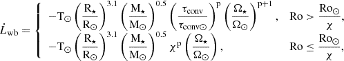
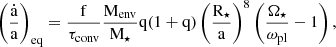
where R⊙ and M⊙ are the radius and mass of the Sun; R⋆ and M⋆ are the radius and mass of the considered star; τconv is the convective turnover timescale (see Eq. (6)); Ro is the stellar Rossby number, defined as the ratio between the star’s rotational period (Prot) and τconv; and Ro⊙ is the solar Rossby number. The braking constant T⊙ = 8 × 1030 erg is calibrated to reproduce the surface-rotation rate of the Sun, and the coefficient p is taken as equal to 2.1. The quantity χ ≡ Ro⊙/Rosat indicates the critical rotation rate for stars with a given τconv/τconv⊙, defining the transition from the saturated to unsaturated regime. In this work, χ is considered equal to 13 (Pezzotti et al. 2021). For what concerns the braking of the stellar surface by magnetised stellar winds, it is possible to account for the onset of a ‘weakened-magnetic-braking’ regime (van Saders et al. 2016) when the stellar Rossby number (Ro) is equal to a critical value of Rocri = 0.92 Ro⊙ (Metcalfe et al. 2024): once a star enters this regime, the efficiency of the braking at its surface is hampered by a shift in the morphology of the magnetic field, from larger to smaller spatial scales (Réville et al. 2015; Garraffo et al. 2016), and (or) by an abrupt change in the mass-loss rate (Ó Fionnagáin & Vidotto 2018). In our code, we account for this effect by simply turning off the magnetic braking component in the computation of the surface angular momentum evolution for Rossby numbers larger than Rocri. The component  in Eq. 1 accounts for the exchange of angular momentum between the star and the planetary orbit due to tidal dissipation (Rao et al. 2021), and its equations read as
![$$ \begin{aligned} \dot{L}_{\rm tides} = \mathrm - \left[ \frac{1}{2} M_{pl} \left( \dfrac{\dot{a}}{a} \right)_{\rm tides} \right] \times \sqrt{\mathrm{G\left( M_{\star } + M_{pl}\right) a}}, \end{aligned} $$](/articles/aa/full_html/2025/02/aa52580-24/aa52580-24-eq11.gif)
where the term  indicates the net variation of the planetary orbital distance (a) due to tidal dissipation (see Eq. (5), (7)), Mpl is the planetary mass, and G is the universal gravitational constant.
2.2.2. Tidal interaction
In our code, star-planet interactions related to the dissipation of equilibrium and dynamical tides within the stellar convective envelope are considered, which can lead to planetary migration through the transfer of angular momentum from the planetary orbit to the stellar surface. In the hypothesis that the planet is on a circular, coplanar orbit around the host star, the net change of its orbital distance can be written as
where the first term is related to planetary mass loss due to photoevaporation, assuming that the mass is lost in space and does not contribute to the exchange of angular momentum between the star and the planetary orbit. The last two terms refer to the contribution of equilibrium and dynamical tides, respectively. Equilibrium tides are most efficiently dissipated in low-mass stars’ convective envelopes due to turbulent friction induced by convection, while their damping is less efficient in other regions (Zahn 1966, 1977). In our approach, we therefore only account for the dissipation of equilibrium tides in convective envelopes, and the equation accounting for their contribution reads as
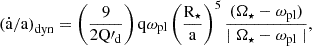
where a is the orbital distance, ȧ is its derivative with respect to time, Menv is the mass contained in the stellar convective envelope, q is the ratio between planetary and stellar mass, Ω⋆ is the host star’s surface-rotation rate, ωpl is the orbital frequency, and R⋆ is the stellar radius. The term τconv is the convective turnover timescale, computed as in Rasio et al. (1996):
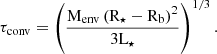
where Rb is the radius at the bottom of the convective envelope and L⋆ is the bolometric luminosity of the host star. The term f in Eq. (5) is a numerical factor obtained from integrating the viscous dissipation of the tidal energy across the convective zone (Villaver & Livio 2009), which is f = (Porb/2τconv)2 (Goldreich & Nicholson 1977) when τconv < Porb/2, otherwise f = 1.
Contrarily to equilibrium tides, dynamical tides might be efficiently dissipated in both convective and radiative regions, depending on the stellar and planetary companion properties. In convective regions, they are excited in the form of inertial waves driven by the Coriolis force whenever the tidal frequency (ωt) ranges between [−2Ω⋆,2Ω⋆] (Ogilvie & Lin 2007). We account for the impact of dynamical tides in convective envelopes in the form of a frequency-averaged tidal dissipation of inertial waves (Ogilvie 2013; Mathis 2015; Bolmont & Mathis 2016). In particular, we assume a two-layer model (core-envelope) in which each of them is characterised by a uniform density (Mathis 2015). If the planet is on a circular-coplanar orbit, dynamical tides are active whenever ωpl < 2Ω⋆ (Ogilvie & Lin 2007), where ωpl is the orbital frequency of the planet. The equation describing the contribution of this type of tides on the evolution of the planetary orbital distance reads as
with Q′d = 3/(2Dω) (modified tidal dissipation factor) and 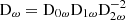 . The ‘D’ terms are defined as follows:
where α = Rb/R⋆, β = Mb/M⋆,  , and
, and  . The terms Mb and Rb are the mass and the radius of the radiative core, considered as the region of the star below the base of the convective envelope. The term Dω is the frequency-averaged tidal dissipation (Ogilvie 2013). We notice that assuming this schematic stratification for the stellar structure, together with the use of a frequency-averaged dissipation rate for the dynamical tide, adds a certain degree of uncertainty to our results. Nevertheless, while this approach suffers from some schematic simplifications, it has the advantage of providing us with relevant orders of magnitude of tidal dissipation rates accounting for the evolution of the structural and rotational parameters of the host star (Mathis 2015; Bolmont & Mathis 2016; Rao et al. 2018; Barker 2020).
In general, for the formalism treated above, tides widen (respectively shrink) the planetary orbit when it is beyond (respectively inside) the corotation radius, which is defined as the distance at which the orbital and host star rotational periods are equal, namely:
![$$ \begin{aligned} \mathrm{a}_{\mathrm{cor}} = \left[ \mathrm{G }\left( \mathrm{M}_{\star } + \mathrm{M}_{\mathrm{pl}} \right)/ \Omega _{\star }^2 \right]^{\frac{1}{3}} .\end{aligned} $$](/articles/aa/full_html/2025/02/aa52580-24/aa52580-24-eq21.gif)
Here, G is the universal gravitational constant, and M⋆ is the mass of the host star. Concerning the formalism used in this work for dynamical tides in the stellar convective envelope, these are efficiently excited in the form of inertial waves when the planetary orbital distance is larger than a minimum critical value, which is defined as  (Ogilvie & Lin 2007).
In the case of early G-type and late F-type stars, a convective core is present in addition to the envelope during the MS and is separated by a radiative region. Nevertheless, dynamical tides excited in convective cores are weakly dissipated. In this case indeed, inertial waves would propagate in a fully convective sphere (the inner core), without the possibility to reflect and lead to the formation of shared wave attractors, which may induce strong dissipation (Ogilvie & Lin 2007, 2004). The dissipation of inertial waves in convective cores is thus not considered in our SPI code.
In general, dynamical tides might also be excited in stellar radiative regions in the form of gravity waves and cause the migration of planets by means of thermal, (weakly) non-linear, or resonance-locking dissipative effects (Goodman & Dickson 1998; Barker & Ogilvie 2010; Weinberg et al. 2012; Ivanov et al. 2013; Essick & Weinberg 2016; Fuller 2017; Ma & Fuller 2021). For solar-type stars with radiative cores, the most likely dominant mechanisms for the dissipation of tidally excited gravity waves are non-linear dissipation, triggered by planetary companions with mass Mp ≳ 0.3 MJ (Essick & Weinberg 2016); or wave breaking, whose triggering requires the planetary mass to be larger than a critical value, which strongly varies as a function of the stellar age from ∼ 102 − 103 MJ at t⋆ ∼ 108 yr to ∼ 10−1 − 10−2 MJ at t⋆ ∼ 1010 yr for a 1 M⊙ star (Barker 2020; Lazovik 2021).
Stars slightly more massive than the Sun (1.1 ≲ M⋆/M⊙ ≲ 1.6) are generally characterised by a rather complex structure on the MS, which is composed of an inner convective core surrounded by a radiative region topped by a shallow convective envelope. In this configuration, the tidally excited gravity waves that travel from the radiative-convective interface towards the stellar centre are reflected at the convective core interface, typically resulting in inefficient dissipation (Barker 2020). An alternative scenario has been proposed for the efficient dissipation of gravity waves propagating in such mixed cores, which consist of the conversion of gravity waves into magnetic waves (Lecoanet et al. 2017, 2022; Rui & Fuller 2023). In this context, tidally excited gravity waves travelling from the radiative-convective envelope boundary towards the stellar centre – upon encountering a sufficiently strong magnetic field generated by the dynamo at work in the convective core – would be fully converted into outwardly propagating magnetic waves; finally, they would be dissipated by radiative or ohmic diffusion (see Duguid et al. 2024, and references therein). By using stellar models with initial masses between 1.2 and 1.6 M⊙, Duguid et al. (2024) showed that the wave conversion mechanism may operate for a significant fraction (of the order of gigayears) of stars’ MS lifetimes. This happens whenever the local radial magnetic field in proximity of the convective core is larger than a critical value at which the radial wave number of tidally excited gravity waves and magnetic waves match (Fuller et al. 2015; Lecoanet et al. 2017, 2022; Rui & Fuller 2023). Differently from the wave-breaking mechanism, wave conversion does not require a plantet’s minimum-mass threshold to be triggered. Another promising dissipation mechanism of tidal gravity waves in this type of star is tidal resonance-locking, in which a planet locks into resonance with a tidally excited stellar gravity mode. This process, similarly to the wave conversion one, can operate for planets of any mass in stars with convective cores (Ma & Fuller 2021).
It is worth stressing that all the tidal excitation and dissipation processes mentioned above strongly depend on the structural and rotational properties of the host star and on its age. The significant uncertainties derived in Sect. 2.1 on the mass, age, and initial chemical composition of GJ 504 – essentially due to a lack of asteroseismic constraints – make it difficult to understand which tidal excitation mechanism might have dominated its past evolution in the hypothetical presence of a close-by planetary companion. While the last two mechanisms mentioned above could have played a major role in this sense, given that GJ 504 could harbour an inner convective core according to our best-fit model, in this work we solely focused on the impact of equilibrium and dynamical tides dissipated within the stellar convective envelope, and we leave the investigation of the impact of tides dissipated in the radiative regions to a future work.
2.2.3. Radiative interaction
In the SPI code, it is possible to compute the erosion of the planetary atmosphere due to the impact of stellar X-ray and extreme ultraviolet (EUV) flux (e.g. Watson et al. 1981; Lammer et al. 2003; Jin et al. 2014). The evolution of the X-ray luminosity is computed by carrying out a recalibration of the Rx-Ro relationship of Johnstone et al. (2021) as in Pezzotti et al. (2021), where Rx = LX/LBol is the ratio between the X-ray luminosity and the bolometric one, while Ro is the stellar Rossby number. The LX and Prot evolution are tightly linked by means of the dynamo-activity-rotation feedback loop (e.g. Parker 1955; Wilson 1966; Kraft 1967); therefore, it is important to simultaneously compute these two quantities. For the computation of the EUV flux, we referred to Johnstone et al. (2021).
Depending on the planetary and system properties, the mass-loss rate from the planet may be computed either by using an energy-limited formula (Watson et al. 1981; Erkaev et al. 2007), in which the factor accounting for the evaporation efficiency is estimated by following Salz et al. (2016) or Caldiroli et al. (2022) or by interpolating (eventually extrapolating) the grid of upper-atmosphere models of Kubyshkina et al. (2018), Kubyshkina & Fossati (2021). Regarding the computation of the planetary radius, depending on the initial mass, fraction of atmosphere, and composition, we used fitting formulae from Lopez & Fortney (2014), Chen & Rogers (2016) or mass-radius relations (Otegi et al. 2020; Bashi et al. 2017). For the range of planetary masses considered in this work, we used Bashi et al. (2017).
3. Analysis of the X-ray data from eROSITA
3.1. Method and tools
We looked for X-ray detections of GJ 504 in the five all-sky surveys of eROSITA (eRASS; Merloni et al. 2024) using the tool EROSE provided by the German consortium. First, we retrieved the sky map where the source is located during the five surveys. Then, we performed the source detection using the eSASSusers_240410 software release (Brunner et al. 2022) within the 0.2 − 5.0 keV energy band, which is usually adopted for M dwarfs (Magaudda et al. 2022). We compiled the list of the detected sources for each of the five surveys using the dedicated eSASS pipeline, ERMLDET, for which we used a threshold detection maximum likelihood of 6.0. Finally, we propagated the Gaia-DR3 coordinates of GJ 504 for their proper motion and at the epoch of the five eROSITA surveys and cross-matched within 10″ these coordinates with those in the result of our source detection. The results are shown in Table 1, where we present the eROSITA survey to which the observation refers (col. 1); the actual observational period of GJ 504 (col. 2); the separation between the proper-motion-corrected coordinates and the X-ray source position from eROSITA (col. 3); the number of source counts with the detection likelihood (cols. 4 and 5); and the source count rate (col. 6).
eROSITA observation log of GJ 504.
3.2. eROSITA spectral analysis
We created the spectrum (shown in Fig. 2), response matrix, and ancillary file for each eROSITA detection using the SRCTOOL pipeline with the AUTO option for the choice of the source and background region sizes. We grouped each spectrum with ten photons per channel for all eRASS, except for eRASS 1 & 5, for which we adopted 15 photons per channel. We fitted the four spectra with XSPEC version 12.13 (Arnaud 1996), adopting the XSPEC library for the stellar abundances compiled by Asplund et al. (2009). We used a one-temperature thermal APEC model with global coronal abundance (Z) fixed at 0.3 Z⊙, as it is typically considered for stellar coronae (Maggio et al. 2007). We calculated the model-dependent X-ray fluxes with the dedicated XSPEC pipeline FLUX initially adopting the eROSITA energy band. For a consistent comparison with the X-ray luminosity from ROSAT (Voges et al. 1999), we also performed a calculation in the ROSAT energy band (0.1 − 2.4 keV), finding that the difference in emitted flux within the two bands is not significant, as previously shown by Magaudda et al. (2022). We used the model-dependent flux with a Gaia-DR3 distance of 17.58 pc to calculate the X-ray luminosity (Lx). The results of our spectral analysis are summarised in Table 2, where we show the eROSITA survey (col. 1), the coronal temperature, and emission measure with their 1σ uncertainties (cols. 2 and 3), the reduced chi-squared value ( ) with the degrees of freedom (cols. 4 and 5), and the X-ray luminosity in the 0.1 − 2.4 keV energy band. We notice that the X-ray luminosity derived in this work with an average value of 1029.42 erg/s is in line with that of Foster et al. (2022) (1029.4 erg/s).
Best-fit parameters from spectral analysis of GJ 504 eROSITA spectra.
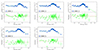 |
Fig. 2. eROSITA spectra of GJ 504 plotted together with best-fitting apec model and the residuals (both shown in green); see text in Sect. 3.2 and Table 2. |
4. Compared evolutionary scenarios: Ωsurf and LX
Once the best-fit model of GJ 504 is computed as described in Sect. 2.1, it is then coupled with our SPI code in order to compute the evolution of the host-star’s surface-rotation rate (Ωsurf) and X-ray luminosity (Lx) in two different evolutionary scenarios: on one hand, we simulate the evolution of the host star by assuming that there is no close-by, massive planet (star without close-by planet; see Sect. 4.1); on the other hand, we assume that a massive planet formed in a short orbit (ain ≤ 0.1 AU) (or migrated close to its host star before the dissipation of the protoplanetary disc), and we studied the impact of its eventual inward migration driven by tidal dissipation and engulfment by the host star on the stellar properties (star with close-by planet; see Sect. 4.2).
With the rotational history of GJ 504 being unknown, we compute models representative of different rotators, from the super-slow to the fast one, using different values for the initial surface-rotation rate (Ωin = 1, 2, 3.2, 5, 6, 7, 8, 9, 10, 18 Ω⊙). Regarding the lifetime of the protoplanetary disc, we considered τdl = 2 Myr for Ωin = 18 Ω⊙ and τdl = 6 Myr for the other values. We recall that the choice of the Ωin and τdl is determined from the distribution of surface-rotation rates observed for stars in star-forming regions and young open clusters at various ages (Eggenberger et al. 2019)4.
4.1. Star without close-by planet (SwoP)
In this evolutionary scenario, we assume that there is no close-by, massive planet orbiting GJ 504. Even if the detection of a sub-stellar companion through direct imaging was announced by Kuzuhara et al. (2013), with a mass of 1 ≲ Mc/MJ ≲ 25, this object is too far away from its host star (≈43.5 AU) to have any significant impact on the evolution of its surface-rotation rate and X-ray luminosity, at least according to the physics included in our SPI code. In this context, in Fig. 3 we collect the results obtained in terms of evolution of the surface-rotation rate, stellar Rossby number, and X-ray luminosity.
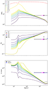 |
Fig. 3. Host star’s evolutionary tracks in the SwoP scenario. Top panel: Surface-rotation-rate evolution versus age for our optimal stellar model, with Ωin = 1, 2, 3.2, 4, 5, 6, 7, 8, 9, 10, 18 Ω⊙. The dashed red line shows the evolution of the critical rotation velocity (Ωcrit), defined as the velocity at which the centrifugal acceleration at the equator equals the gravity. The magenta and black markers show GJ 504’s surface rotation rate, with age uncertainties derived from the global and local minimisation modelling, respectively. Middle panel: Evolution of stellar Rossby number (RO). RO for GJ 504 is indicated by the red, black, and blue circles corresponding to the lower, mean, and upper values of the largest age uncertainty, respectively. The grey and black stars represent the values obtained from τconv as in Wright et al. (2011) and Wright et al. (2018). Analogously, the magenta markers represent the same quantities for the smallest age uncertainty. Bottom panel: Evolution of X-ray luminosity for each of the considered rotators. The black and blue markers show the X-ray luminosities from Voges et al. (1999), Wright et al. (2011) (ROSAT) and in this work (eROSITA), respectively. Analogously, the magenta markers represent the same quantities for the smallest age uncertainty. In all panels, the starting point of the tracks corresponds to the dissipation of the protoplanetary disc (2 Myr for Ωin = 18 Ω⊙; 6 Myr for the other ones). |
4.1.1. SwoP: Surface-rotation rate
In the top panel of Fig. 3, we show the evolution of the surface rotation rate normalised to the value of the Sun (Ω⊙ = 2.9 × 10⁻⁶ s−1) for each of the considered rotational histories as a function of the stellar age. As expected in the case of stars without close-by planets, the evolution of the surface-rotation rate is initially governed by the contraction of the stellar radius during the PMS phase until the star reaches the zero-age main sequence (ZAMS) at about 25 Myr. Subsequently, the braking of the stellar surface due to magnetised winds takes over, determining the overlap of the majority of the tracks at ≈500 Myr, except for the 1 Ω⊙ model, which globally evolves at lower values. By comparing the theoretical tracks with the rotation rate derived for GJ 504 in Di Mauro et al. (2022) (Prot = 3.4 days, ΩGJ 504 = 2.13 × 10⁻⁵ s−1), we notice that there is only compatibility if we consider the youngest possible value for the stellar age (0.36 Gyr), and this is only for Ωin ≥ 10 Ω⊙; otherwise, ΩGJ 504 is larger than what was expected from our models.
We analysed whether considering the onset of weakened magnetic braking at Ro = Rocri could result in a better overlapping of the theoretical tracks and the observational data. Because of the impact of this mechanism indeed, the braking of the stellar surface would be stalled after a certain age, leading to larger surface-rotation rates at the age of GJ 504. The trend of the evolutionary tracks in this circumstance, computed only for Ωin = 3.2, 5, 18 Ω⊙, is shown by the dashed grey lines in the top panel of Fig. 3. It is possible to noticed that at the onset of weakened magnetic braking (∼2 Gyr), the star has already been significantly braked, and there is no compatibility with the observational value.
4.1.2. SwoP: Stellar Rossby number
In the middle panel of Fig. 3, the stellar Rossby number evolutionary tracks are presented. To make a comparison with the Rossby number obtained by using Prot = 3.4 d, and given the significant uncertainty on GJ 504 age, we estimated three different RO at the lower, mean, and upper limits of the error bar. Using Eq. (6), we derive ROlow = 0.65, ROm = 0.62, ROup = 0.43. Similarly to what we found for the surface rotation rate, an agreement with the evolutionary tracks was only obtained for the smallest value of the host star ages, namely for ROlow and for Ωin ≥ 10 Ω⊙. It is worth noticing that we used a model-dependent approach to compute the Rossby number by means of Eq. (6) for τconv in order to be consistent with the physics included in the SPI code. However, it is possible to compare our estimation of τconv with the values derived by prescriptions based on purely observational properties. This is the case of the formulae in Wright et al. (2011, 2018) based on the (V − KS) colour, which were calibrated on a sample of solar and late-type MS stars. In order to make a comparison with our model-dependent convective turnover timescale computation, we used Eq. (10) from Wright et al. (2011) and Eq. (5) in Wright et al. (2018), with (V − KS) = 1.29 (Wright et al. 2011). We finally obtain τconvW11 = 10.3228 d and τconvW18 = 9.1727 d. In Fig. 4, we compare these two values with the evolutionary track. At ≈2.11 Gyr, there is a difference of about 8 d between the purely observational and theoretical estimations of τconv. Consequently, the corresponding Rossby numbers also show significantly diverse values in the middle panel of Fig. 3, where ROm = 0.62, ROW11 = 0.33 and ROW18 = 0.37.
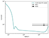 |
Fig. 4. Comparison between convective turnover timescale obtained from CLES best-fit model using Eq. (6), and the values computed as in Wright et al. (2011) (grey star) and Wright et al. (2018) (black star). |
In the same panel, we also indicate the value of the critical Rossby number (ROcri, dotted black line, Metcalfe et al. 2024), above which the star may transition to the weakened magnetic braking regime (van Saders et al. 2016). According to our theoretical models, a star such as GJ 504 would cross ROcri at an age of ∼1 − 2 Gyr. As mentioned in the previous sections, at this point the star has been significantly braked by the magnetised winds to values well below ΩGJ504. Thus, magnetic braking seems not to be responsible for the faster rotation of the star.
4.1.3. SwoP: X-ray luminosity
In the bottom panel of Fig. 3, the X-ray luminosity tracks are shown. Each track corresponds to a different rotational history. We compare the tracks with observational data from Voges et al. (1999), Wright et al. (2011) for ROSAT – with LX = 1029.47 erg/s (black dot) – and from our analysis of eROSITA, from which we derive an average value of LX = 1029.42 erg/s. Differently than what we observed for Ω and Ro, in this case an agreement between the theoretical tracks and the observed value is not observed, even for the lowest age value allowed for GJ 504. It is worth recalling that low and solar-like stars may experience significant variations in the emission of X-ray luminosity (over one order of magnitude), which are usually linked with the periodicity of their magnetic cycle.
4.2. Star with close-by planet (SwP)
In the star-with-close-by-planet scenario, we test the impact of the inward migration of a giant planet on the surface-rotation rate and X-ray luminosity of the host star, GJ 504. On the basis of analytical considerations, Fuhrmann & Chini (2015) proposed that the minimum mass needed for the planet to reproduce the observed stellar spin up is Mpl ≳ 2.7 MJ. In their work, the authors assumed that the angular momentum of the star is entirely related to the transfer of angular momentum from the planetary orbit, which occurred once the planet had filled its Roche lobe. In this work, we account for the intrinsic angular momentum of the host star together with that transferred by the planetary orbit. We thus studied the impact of equilibrium and dynamical tides dissipated within the host star’s convective envelope on the migration of the planet and its feedback on the stellar surface-rotation rate and X-ray luminosity evolution.
We first explored a range of initial orbital distances (0.02 ≤ a (AU) ≤ 0.1) and planetary masses (1 ≤ Mpl/MJ ≤ 10), and we selected stellar models representative of slow, moderate, and fast rotators – namely Ωin = 3.2, 5, 18 Ω⊙ (Eggenberger et al. 2019) – to find for which combination the computed stellar rotational period and X-ray luminosity are compatible with the observed values. In Fig. 5, we show the corresponding results. From these computations, we find that for the slow and moderate rotators it is possible to determine a region of compatibility in the a − Mpl plane, which is indicated by the black hatched area in the top and middle panels of Fig. 5. Contrarily, for the fast rotator case this compatibility is not retrieved. In this case, the planetary engulfment generally occurs at too early evolutionary stages (∼4 Myr), when the star is spinning up due to its contraction in the PMS; thus, the contribution to the stellar angular momentum is not only less important, but also quickly erased by subsequent magnetic braking. A further difference between the slow-moderate and fast rotators is that while in the first two cases the orbit of the planet shrinks for 0.03 ≲ a(AU) ≲ 0.06, in the last one the orbit expands for 0.025 ≲ a(AU) ≲ 0.1. This is due to the different geometry of the corotation radius (acor) and, consequently, amin, which at the beginning of the evolution is smaller for larger values of Ωin (see Eq. (9)). To clarify this point, in Fig. 6 we show an example of orbital evolution for a 1 MJ planet with ain = 0.02, 0.025, 0.03, 0.035, 0.04, 0.06, 0.08, 0.1 AU, and Ωin = 3.2, 18 Ω⊙. In the slow rotator case, most of the tracks (ain ≤ 0.06 AU) begin the evolution below amin; thus, dynamical tides are not at work, and the orbit of the planet remains constant. Given that the initial surface-rotation rate of the star is quite low and the efficiency of tidal dissipation is tightly linked with this quantity, even after crossing amin at about 10 − 20 Myr the orbit is not significantly affected by dynamical tides. Equilibrium tides finally deflect the orbit for ain = 0.02, 0.025 AU at ∼2 Gyr, making the planet migrate towards its host star, since ain < acor. It is worth noting that we followed the evolution of the planet until it reached its Roche limit5 (Zhang & Penev 2014). Following Benbakoura et al. (2019), at this point we assume that it is instantaneously depleted by tidal interactions and transfers its orbital angular momentum to the host star. As indicated in Metzger et al. (2012), when the ratio between the planetary and stellar density is in the 1 < ρpl/ρ⋆ < 5 range and the planet overflows its Roche lobe, an unstable mass transfer takes place, tearing apart the planet within a timescale of several hours. For the range of planetary masses considered here, for the slow and moderate rotators, the ratio ρpl/ρ⋆ at the engulfment (∼2 Gyr) is about 2–3. Thus, the assumption of instantaneous planetary disruption seems to be reasonable. Concerning the fast rotator case, as shown in Fig. 6, dynamical tides are much more efficiently dissipated, and planets starting the evolution below the corotation radius quickly migrate towards the host star, reaching the Roche limit. At this evolutionary stage, the ratio ρpl/ρ⋆ > 5, and, according to Metzger et al. (2012), the planet would spiral and finally plunge into the stellar atmosphere. This event probably lasts more than the aforementioned instantaneous depletion. Even if we assume an instantaneous angular momentum transfer, to maximise its effect, given that the star is still spinning up at this stage it does not significantly impact the rotational evolution of its surface (at least according to the physics included in this work). Planets starting their evolution above the corotation radius (0.025 < ain (AU) < 0.08) are instead pushed outwards.
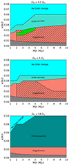 |
Fig. 5. Different orbital evolutions for a planet with 1 ≤ Mplin/MJ ≤ 10 and 0.02 ≤ ain (AU) ≤ 0.1 computed for Ωin = 3.2 Ω⊙ (top panel), Ωin = 5 Ω⊙ (middle panel), and Ωin = 18 Ω⊙ (bottom panel). The salmon-coloured hatched area shows the parameter space for which, after the engulfment, it is possible to reproduce the rotational period and X-ray luminosity of GJ 504 when considering the largest age uncertainty. The lime-hatched area indicates a subset of the salmon-hatched area, for the smaller age uncertainty. The grey shaded area shows the region below the Roche limit. |
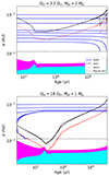 |
Fig. 6. Orbital evolution for 1 MJ planet with 0.02 ≤ ain (AU) ≤ 0.1 and Ωin = 3.2, 18 Ω⊙ (top and bottom panels, respectively). The solid blue lines show the evolution of the orbital distance. The dotted red and dashed black lines indicate the evolution of amin and acor, respectively. The Roche limit is shown by the black dotted line. The cyan and magenta shaded areas represent the extension of the stellar core and envelope along the evolution of the star, respectively. |
In the contextof the orbital evolution, we computed the mass loss from the planet due to the stellar XUV flux. Given the large planetary masses considered in these simulations, the mass loss due to the stellar high energy irradiation turns out to be negligible (e.g. Owen & Wu 2013).
After exploring the parameter space in Mpl, ain, and Ωin, in the following we focus on studying the orbital evolution of a planet with a mass of 3 MJ, which was arbitrarily chosen in the range of compatibility, and with ain = 0.025 AU, for which we analyse a finer grid in Ωin = 1, 2, 3.2, 5, 6, 7, 8, 9, 10, 18 Ω⊙, as for the star-without-close-by-planet scenario. The goal is to investigate for which range of rotational histories the simulations reproduce the observed Prot and LX. The corresponding results are shown in Fig. 76.
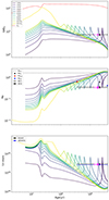 |
Fig. 7. Host star’s evolutionary tracks in the SwP scenario. Evolution of stellar surface-rotation rate (top panel), stellar Rossby number (middle panel), and X-ray luminosity (bottom panel) under the impact of planetary inward migration. For the stellar initial surface-rotation rate, we considered the following values: Ωin = 1, 2, 3.2, 4, 5, 6, 7, 8, 9, 10, 18 Ω⊙. For the planetary mass, we considered Mpl = 3 MJ, and for the initial planetary orbital distance, we considered ain = 0.025 AU. The meaning of the other quantities is the same as in Fig. 3. |
It is worth recalling that the results found in this section rely on the assumption that the planet formed (or migrated before the dispersal of the planetary disc) very closely to the host star, sitting on a coplanar-circular orbit. However, other mechanisms could have brought the planet to a very short orbit after its formation, with an initial planetary architecture characterised by a certain inclination and eccentricity. In particular, the presence of sub-stellar companion (at a projected distance of ∼43.5 AU) could have triggered the inner planet’s orbital shrinking by means of plant-planet scattering (e.g. Rasio & Ford 1996) and (or) Kozai-Lidov oscillations (Kozai 1962; Lidov 1962; Mazeh et al. 1997). The latter consists of a dynamical mechanism affecting the orbit of the inner planet with a periodically exchanging variation between its eccentricity and inclination. The excitation of the planetary eccentricity by means of these processes, together with tidal dissipation within the inner planet at every passage at the periastron, would potentially relocate the planet to a much shorter and circular orbit, which would eventually be short enough to induce tidal dissipation in the stellar host. In a more extreme scenario, for relatively large eccentricity values the planet could be directly engulfed at one of its periastron passages. Depending on the properties of the perturber, the initial orbital parameters of the system, and the structure of the inner planet, the timescales for these mechanisms to be triggered and result in an efficient planetary engulfment and spin-up of the host star might significantly vary. In the case of GJ 504, given the limited constrains available on the system properties, it is challenging to establish whether planet-planet scattering and (or) Lidov-Kozai oscillations could be triggered. Since stellar tides could still play a major role in a scenario when also considering these two processes, future simulations accounting for this mechanism could benefit from the results found in this work.
4.2.1. SwP: Surface-rotation rate
In the top panel of Fig. 7, we show the evolution of the stellar surface-rotation rate for each of the considered rotational histories as a function of the stellar age. As for the star-without-close-by-planet scenario, the PMS phase is dominated by the structural contraction until the star reaches the ZAMS, at which point the magnetic braking takes over. Since the planetary companion orbits very closely to the host star, because of the impact of equilibrium and dynamical tides, it migrates inwards. The majority of the orbital angular momentum is transferred to the star when the planet reaches the closest orbits to the Roche limit, and thus the star experiences a kick that results in a spike in the Ω vesus Age track. For Ωin ≥ 3.2 Ω⊙, the larger the value of Ωin, the earlier the engulfment of the planet occurs. On the contrary, for Ωin < 3.2 Ω⊙ – since the orbital migration is only driven by equilibrium tides – the engulfment occurs at approximately the same age (∼2.5 Gyr). As mentioned above, for the fastest rotator considered here (18 Ω⊙), the planet is engulfed during the PMS, and the angular momentum transferred from the planetary orbit does not contribute significantly to the global one of the star. This is shown from the yellow track in the top panel of Fig. 7, where at the moment of the engulfment (∼10 Myr) only a small increase of Ω is visible. For the other rotators, the planetary engulfment induces a stellar spin-up to about 11 − 12 Ω⊙. The quasi-vertical increase of the surface-rotation rate is followed by a smoother decay, driven by the magnetic braking. Given that the timescale of the rotation-rate decay is larger than the spin-up one, if a planetary engulfment caused the acceleration of GJ 504, it is more probable that we are observing the star in the decelerating phase. In the less likely hypothesis that the planet has not been engulfed yet, but it is at the edge of its Roche limit, in transferring its angular momentum to the star, we can try to estimate the radial-velocity (RV) semi-amplitude signal induced on its host. Using Eq. (1) of Cumming et al. (1999), by considering the lowest initial mass required for the compatible companion to reproduce the observed Prot and LX for GJ 504, namely 2 MJ, the line-of-sight inclination from Bonnefoy et al. (2018) (i = 18.6 degrees), and an orbital distance of ain = 0.01 AU (Porb = 8 d), we obtain K = 52.18 m/s. D’Orazi et al. (2017) ruled out the presence of a massive companion close enough to tidally spin up the central star on the basis of RV monitoring performed at Lick Observatory (Fischer et al. 2014). The observed RV dispersion in this case is 25.7 m/s, which may be comparable to the activity level of the star. They thus excluded the presence of close-by companions more massive than 0.5 − 1 MJ. Nevertheless, if the planet is undergoing tidal destruction when crossing the Roche limit, the actual RV semi-amplitude could be much smaller than the ∼52 m/s estimated above, since it would only be caused by some planetary remnants at this stage. As reported in D’Orazi et al. (2017), this would require purposely designed observations.
In terms of compatibility between the observational value for the surface rotation rate and the evolutionary tracks, if we look at the decaying branches for each Ωin, it is possible to narrow down the initial surface-rotation rate to values ≤10 Ω⊙. It is worth noting that the overlap between the evolutionary tracks and the observational Ω⋆ would favour ages between 360 Myr and 3 Gyr (approximately), while no overlap is obtained for older ages.
4.2.2. SwP: Stellar Rossby number
Once the star is spun up by the planetary engulfment, its Rossby number decreases. This is presented in the middle panel of Fig. 7, where for each of the considered rotators the Rossby number sharply decreases when the planet reaches its Roche limit. In this context, the tracks predict smaller values of RO, which become compatible with both ROm and ROup, even though the maximum age for compatibility is ∼3 Gyr, as for the surface-rotation rate. Better compatibility is also observed with the Rossby number computed by means of the Wright et al. (2011, 2018) formulae.
4.2.3. SwP: X-ray luminosity
The final comparison between the X-ray luminosity tracks and the observational data obtained from ROSAT (Voges et al. 1999; Wright et al. 2011) and eROSITA are shown in the bottom panel of Fig. 7. Very interestingly, with the engulfment of a massive enough planet (Mpl ≥ 2 MJ) and for Ωin ≲ 7 Ω⊙, an overlapping of the tracks and the observational data is retrieved. Conversely to the comparison with the surface-rotation rate, the interval for the possible values of Ωin compatible with LXGJ504 is narrower. Therefore, in order to simultaneously reproduce both the rotational period and X-ray luminosity of GJ 504, the initial surface-rotation rate of the star should be ≤7 Ω⊙.
5. Conclusion
In this work, we studied the properties of GJ 504 and investigated whether with the engulfment of a planetary companion the observed surface rotation rate and X-ray luminosity can be reproduced. On the basis of the best-fit stellar model of GJ 504 derived by means of a two-step minimisation technique, and by using our SPI code, we computed tracks for the stellar surface-rotation rate and X-ray luminosity assuming two evolutionary scenarios: star without close-by planet, in which there is no close-by companion influencing the evolution of the star; and star with close-by planet, in which a massive planet orbits closely and migrates inwards due to tides dissipated within the host star. The rotational history of the star being unknown, we selected a broad range of initial surface-rotation rates, from super-slow (1 Ω⊙) to fast-rotator (18 Ω⊙). When comparing the tracks obtained in the star-without-close-by-planet evolutionary scenario, we find that there is only compatibility with the surface-rotation rate of GJ 504 for Ωin ≥ 10 Ω⊙, within the considered age range (0.36 − 3.86) Gyr. There is no compatibility with the observed X-ray luminosity, for which the tracks predict smaller values.
In the star-with-close-by-planet scenario, we initially explored the parameter space in planetary initial mass (1 ≤ Mpl(MJ)≤10), orbital distance (0.02 ≤ ain(AU)≤0.1), and host-star surface-rotation rate (Ωin = 3.2, 5, 18 Ω⊙) to find the set of conditions needed for the planet to efficiently spin up the star after the engulfment. As a result, we find that for Mpl ≥ 2 MJ, 0.02 ≤ ain(AU) ≤ 0.035 and host star Ωin < 18 Ω⊙, the engulfed planet is able to spin up the host star to values compatible with both the surface-rotation rate and X-ray luminosity observed for GJ 504.
Given the broad range of the considered host-star surface-rotation rates, within the aforementioned parameter space we arbitrarily focused on studying the orbital evolution of a 3 MJ planet, at ain = 0.025 AU, and a finer grid in Ωin = 1, 2, 3.2, 5, 6, 7, 8, 9, 10, 18 Ω⊙, with the aim of breaking down the degeneracy on the GJ 504 initial surface-rotation rate. In this star-planet configuration, we find that the surface-rotation rate and X-ray luminosity of GJ 504 can be both reproduced for Ωin ≤ 7 Ω⊙. Moreover, for 3.2 ≤ Ωin/Ω⊙ ≤ 7, the larger the initial surface-rotation rate, the earlier the engulfment occurs. An interesting result is that the overlap between the evolutionary tracks and the observational Ω⋆ seems to favour ages between 360 Myr and 3 Gyr for GJ 504, approximately, while no overlap is obtained for older ages. In Appendix B, we show the results obtained by doing a similar exercise, but this time we fixed Ωin = 3.2 Ω⊙ and let the initial orbital distance vary between 0.02 and 0.1 AU. Analogously to what was found above, the shorter the initial orbital distance, the earlier the engulfment occurs. Moreover, in this case the overlap between the tracks and the observational values also tends to favour ages for GJ 504 up to ∼2.5 Gyr. These results clearly show that despite the fact we managed to determine a region in Mpl-ain-Ωin within which the theoretical tracks are compatible with the observational constraints for GJ 504, the problem still remains strongly degenerate.
According to the two evolutionary scenarios analysed in this work, only the star-with-close-by-companion one is able to produce tracks compatible with both the surface-rotation rate and X-ray luminosity of GJ 504, which results to be a strong candidate for a star that underwent strong star-planet interactions. It is interesting to notice that the planetary inward migration and consequent destruction at the Roche limit should have occurred late enough in the MS, otherwise the braking at the stellar surface due to magnetised winds would easily have erased any trace of spin-up.
It is worth stressing that despite the fact that our work supports the engulfment scenario as a means to reconcile the age estimation discrepancies between activity indicators and classical parameters, thus favouring a more evolved evolutionary stage for GJ 504, the problem of deriving accurate stellar parameters remains. This will be crucial to establishing the nature of GJ 504 and characterising the impact of SPI. In this context, asteroseismology is the only tool able to address this need. Future observations with TESS in the announced ultra-short cadence mode in the extended campaign might open up the opportunity of detecting solar-like oscillations.
Typically, in Eggenberger et al. (2019) the values Ωin = 3.2, 5, 18 Ω⊙ correspond to the slow, moderate, and fast rotators, respectively.
For the sake of completeness, in Appendix A we present similar results obtained this time for a 1 MJ planet with ain = 0.02 AU, showing that there is compatibility between the theoretical and observational values for the rotational period, but not for the X-ray luminosity.
Acknowledgments
We thank the reviewer Dr. Yaroslav Lazovik for his thorough and helpful comments, that helped to improve the quality and clarity of the manuscript. CP thanks the Belgian Federal Science Policy Office (BELSPO) for the financial support in the framework of the PRODEX Program of the European Space Agency (ESA) under contract number 4000141194. GB is funded by the Fonds National de la Recherche Scientifique (FNRS). EM is supported by Deutsche Forschungsgemeinschaft under grant STE 1068/8-1. This work is based on data from eROSITA, the soft X-ray instrument aboard SRG, a joint Russian-German science mission supported by the Russian Space Agency (Roskosmos), in the interests of the Russian Academy of Sciences represented by its Space Research Institute (IKI), and the Deutsches Zentrum für Luft- und Raumfahrt (DLR). The SRG spacecraft was built by Lavochkin Association (NPOL) and its subcontractors, and is operated by NPOL with support from the Max Planck Institute for Extraterrestrial Physics (MPE). The development and construction of the eROSITA X-ray instrument was led by MPE, with contributions from the Dr. Karl Remeis Observatory Bamberg & ECAP (FAU Erlangen-Nuernberg), the University of Hamburg Observatory, the Leibniz Institute for Astrophysics Potsdam (AIP), and the Institute for Astronomy and Astrophysics of the University of Tübingen, with the support of DLR and the Max Planck Society. The Argelander Institute for Astronomy of the University of Bonn and the Ludwig Maximilians Universität Munich also participated in the science preparation for eROSITA. The eROSITA data shown here were processed using the eSASS/NRTA software system developed by the German eROSITA consortium. VVG is an F.R.S.-FNRS Research Associate. SB acknowledges funding from the Dutch Research Council (NWO) with project number OCENW.M.22.215 of the research program ‘Open Competition Domain Science- M’.
References
- Adibekyan, V., Sousa, S. G., & Santos, N. C. 2018, in Asteroseismology and Exoplanets: Listening to the Stars and Searching for New Worlds, eds. T. L. Campante, N. C. Santos, & M. J. P. F. G. Monteiro, Astrophys. Space Sci. Proc., 49, 225 [NASA ADS] [CrossRef] [Google Scholar]
- Arnaud, K. A. 1996, in Astronomical Data Analysis Software and Systems V, eds. G. H. Jacoby, & J. Barnes, Astronomical Society of the Pacific Conference Series, 101, 17 [NASA ADS] [Google Scholar]
- Asplund, M., Grevesse, N., Sauval, A. J., & Scott, P. 2009, ARA&A, 47, 481 [NASA ADS] [CrossRef] [Google Scholar]
- Barker, A. J. 2020, MNRAS, 498, 2270 [Google Scholar]
- Barker, A. J., & Ogilvie, G. I. 2010, MNRAS, 404, 1849 [NASA ADS] [Google Scholar]
- Barnes, S. A. 2007, ApJ, 669, 1167 [Google Scholar]
- Bashi, D., Helled, R., Zucker, S., & Mordasini, C. 2017, A&A, 604, A83 [NASA ADS] [CrossRef] [EDP Sciences] [Google Scholar]
- Benbakoura, M., Réville, V., Brun, A. S., Le Poncin-Lafitte, C., & Mathis, S. 2019, A&A, 621, A124 [NASA ADS] [CrossRef] [EDP Sciences] [Google Scholar]
- Benomar, O., Takata, M., Shibahashi, H., Ceillier, T., & García, R. A. 2015, MNRAS, 452, 2654 [Google Scholar]
- Benomar, O., Bazot, M., Nielsen, M. B., et al. 2018, Science, 361, 1231 [Google Scholar]
- Bétrisey, J., Eggenberger, P., Buldgen, G., Benomar, O., & Bazot, M. 2023, A&A, 673, L11 [NASA ADS] [CrossRef] [EDP Sciences] [Google Scholar]
- Bolmont, E., & Mathis, S. 2016, Celest. Mech. Dyn. Astron., 126, 275 [Google Scholar]
- Bonnefoy, M., Perraut, K., Lagrange, A. M., et al. 2018, A&A, 618, A63 [NASA ADS] [CrossRef] [EDP Sciences] [Google Scholar]
- Brunner, H., Liu, T., Lamer, G., et al. 2022, A&A, 661, A1 [NASA ADS] [CrossRef] [EDP Sciences] [Google Scholar]
- Caldiroli, A., Haardt, F., Gallo, E., et al. 2022, A&A, 663, A122 [NASA ADS] [CrossRef] [EDP Sciences] [Google Scholar]
- Chen, H., & Rogers, L. A. 2016, ApJ, 831, 180 [Google Scholar]
- Cumming, A., Marcy, G. W., & Butler, R. P. 1999, ApJ, 526, 890 [Google Scholar]
- Cuntz, M., Saar, S. H., & Musielak, Z. E. 2000, ApJ, 533, L151 [Google Scholar]
- da Silva, R., Porto de Mello, G. F., Milone, A. C., et al. 2012, A&A, 542, A84 [NASA ADS] [CrossRef] [EDP Sciences] [Google Scholar]
- Di Mauro, M. P., Reda, R., Mathur, S., et al. 2022, ApJ, 940, 93 [NASA ADS] [CrossRef] [Google Scholar]
- Donahue, R. A., Saar, S. H., & Baliunas, S. L. 1996, ApJ, 466, 384 [Google Scholar]
- D’Orazi, V., Desidera, S., Gratton, R. G., et al. 2017, A&A, 598, A19 [CrossRef] [EDP Sciences] [Google Scholar]
- Duguid, C. D., de Vries, N. B., Lecoanet, D., & Barker, A. J. 2024, ApJ, 966, L14 [NASA ADS] [CrossRef] [Google Scholar]
- Eggenberger, P., Buldgen, G., & Salmon, S. J. A. J. 2019, A&A, 626, L1 [NASA ADS] [CrossRef] [EDP Sciences] [Google Scholar]
- Erkaev, N. V., Kulikov, Y. N., Lammer, H., et al. 2007, A&A, 472, 329 [NASA ADS] [CrossRef] [EDP Sciences] [Google Scholar]
- Essick, R., & Weinberg, N. N. 2016, ApJ, 816, 18 [Google Scholar]
- Farnir, M., Dupret, M. A., Buldgen, G., et al. 2020, A&A, 644, A37 [EDP Sciences] [Google Scholar]
- Fellay, L., Pezzotti, C., Buldgen, G., Eggenberger, P., & Bolmont, E. 2023, A&A, 669, A2 [NASA ADS] [CrossRef] [EDP Sciences] [Google Scholar]
- Fischer, D. A., Marcy, G. W., & Spronck, J. F. P. 2014, ApJS, 210, 5 [Google Scholar]
- Foster, G., Poppenhaeger, K., Ilic, N., & Schwope, A. 2022, A&A, 661, A23 [NASA ADS] [CrossRef] [EDP Sciences] [Google Scholar]
- Fuhrmann, K., & Chini, R. 2015, ApJ, 806, 163 [NASA ADS] [CrossRef] [Google Scholar]
- Fuller, J. 2017, MNRAS, 472, 1538 [Google Scholar]
- Fuller, J., Cantiello, M., Stello, D., Garcia, R. A., & Bildsten, L. 2015, Science, 350, 423 [Google Scholar]
- García, R. A., Turck-Chièze, S., Jiménez-Reyes, S. J., et al. 2007, Science, 316, 1591 [Google Scholar]
- Garraffo, C., Drake, J. J., & Cohen, O. 2016, A&A, 595, A110 [NASA ADS] [CrossRef] [EDP Sciences] [Google Scholar]
- Goldreich, P., & Nicholson, P. D. 1977, Icarus, 30, 301 [NASA ADS] [CrossRef] [Google Scholar]
- Goodman, J., & Dickson, E. S. 1998, ApJ, 507, 938 [Google Scholar]
- Holmberg, J., Nordström, B., & Andersen, J. 2009, A&A, 501, 941 [NASA ADS] [CrossRef] [EDP Sciences] [Google Scholar]
- Iglesias, C. A., & Rogers, F. J. 1996, ApJ, 464, 943 [NASA ADS] [CrossRef] [Google Scholar]
- Ilić, N., Poppenhaeger, K., Dsouza, D., et al. 2023, MNRAS, 524, 5954 [CrossRef] [Google Scholar]
- Ilić, N., Poppenhaeger, K., Queiroz, A. B., & Chiappini, C. 2024, Astron. Nachr., 345, e20230132 [Google Scholar]
- Irwin, A. W. 2012, Astrophysics Source Code Library [record ascl:1211.002] [Google Scholar]
- Ivanov, P. B., Papaloizou, J. C. B., & Chernov, S. V. 2013, MNRAS, 432, 2339 [Google Scholar]
- Jin, S., Mordasini, C., Parmentier, V., et al. 2014, ApJ, 795, 65 [Google Scholar]
- Johnstone, C. P., Bartel, M., & Güdel, M. 2021, A&A, 649, A96 [EDP Sciences] [Google Scholar]
- Kozai, Y. 1962, AJ, 67, 591 [Google Scholar]
- Kraft, R. P. 1967, ApJ, 150, 551 [Google Scholar]
- Kubyshkina, D. I., & Fossati, L. 2021, Res. Notes Am. Astron. Soc., 5, 74 [Google Scholar]
- Kubyshkina, D., Fossati, L., Erkaev, N. V., et al. 2018, ApJ, 866, L18 [NASA ADS] [CrossRef] [Google Scholar]
- Kuzuhara, M., Tamura, M., Kudo, T., et al. 2013, ApJ, 774, 11 [Google Scholar]
- Lammer, H., Selsis, F., Ribas, I., et al. 2003, ApJ, 598, L121 [Google Scholar]
- Lazovik, Y. A. 2021, MNRAS, 508, 3408 [NASA ADS] [CrossRef] [Google Scholar]
- Lebreton, Y., & Reese, D. R. 2020, A&A, 642, A88 [NASA ADS] [CrossRef] [EDP Sciences] [Google Scholar]
- Lecoanet, D., Vasil, G. M., Fuller, J., Cantiello, M., & Burns, K. J. 2017, MNRAS, 466, 2181 [Google Scholar]
- Lecoanet, D., Bowman, D. M., & Van Reeth, T. 2022, MNRAS, 512, L16 [NASA ADS] [CrossRef] [Google Scholar]
- Lidov, M. L. 1962, Planet. Space Sci., 9, 719 [Google Scholar]
- Lopez, E. D., & Fortney, J. J. 2014, ApJ, 792, 1 [Google Scholar]
- Ma, L., & Fuller, J. 2021, ApJ, 918, 16 [NASA ADS] [CrossRef] [Google Scholar]
- Magaudda, E., Stelzer, B., Raetz, S., et al. 2022, A&A, 661, A29 [NASA ADS] [CrossRef] [EDP Sciences] [Google Scholar]
- Maggio, A., Flaccomio, E., Favata, F., et al. 2007, ApJ, 660, 1462 [NASA ADS] [CrossRef] [Google Scholar]
- Mathis, S. 2015, A&A, 580, L3 [EDP Sciences] [Google Scholar]
- Matt, S. P., Brun, A. S., Baraffe, I., Bouvier, J., & Chabrier, G. 2015, ApJ, 799, L23 [Google Scholar]
- Matt, S. P., Brun, A. S., Baraffe, I., Bouvier, J., & Chabrier, G. 2019, ApJ, 870, L27 [Google Scholar]
- Mazeh, T., Krymolowski, Y., & Rosenfeld, G. 1997, ApJ, 477, L103 [NASA ADS] [CrossRef] [Google Scholar]
- Merloni, A., Larmer, G., Liu, T., et al. 2024, A&A, 682, A34 [NASA ADS] [CrossRef] [EDP Sciences] [Google Scholar]
- Messina, S., Pizzolato, N., Guinan, E. F., & Rodonò, M. 2003, A&A, 410, 671 [CrossRef] [EDP Sciences] [Google Scholar]
- Metcalfe, T. S., Strassmeier, K. G., Ilyin, I. V., et al. 2024, ApJ, 960, L6 [NASA ADS] [CrossRef] [Google Scholar]
- Metzger, B. D., Giannios, D., & Spiegel, D. S. 2012, MNRAS, 425, 2778 [CrossRef] [Google Scholar]
- Miglio, A., & Montalbán, J. 2005, A&A, 441, 615 [NASA ADS] [CrossRef] [EDP Sciences] [Google Scholar]
- Nielsen, M. B., Schunker, H., Gizon, L., & Ball, W. H. 2015, A&A, 582, A10 [NASA ADS] [CrossRef] [EDP Sciences] [Google Scholar]
- Ó Fionnagáin, D., & Vidotto, A. A. 2018, MNRAS, 476, 2465 [CrossRef] [Google Scholar]
- Oetjens, A., Carone, L., Bergemann, M., & Serenelli, A. 2020, A&A, 643, A34 [NASA ADS] [CrossRef] [EDP Sciences] [Google Scholar]
- Ogilvie, G. I. 2013, MNRAS, 429, 613 [Google Scholar]
- Ogilvie, G. I., & Lin, D. N. C. 2004, ApJ, 610, 477 [Google Scholar]
- Ogilvie, G. I., & Lin, D. N. C. 2007, ApJ, 661, 1180 [Google Scholar]
- Otegi, J. F., Bouchy, F., & Helled, R. 2020, A&A, 634, A43 [NASA ADS] [CrossRef] [EDP Sciences] [Google Scholar]
- Owen, J. E., & Wu, Y. 2013, ApJ, 775, 105 [Google Scholar]
- Parker, E. N. 1955, ApJ, 122, 293 [Google Scholar]
- Pezzotti, C., Eggenberger, P., Buldgen, G., et al. 2021, A&A, 650, A108 [NASA ADS] [CrossRef] [EDP Sciences] [Google Scholar]
- Pillitteri, I., Micela, G., Maggio, A., Sciortino, S., & Lopez-Santiago, J. 2022, A&A, 660, A75 [NASA ADS] [CrossRef] [EDP Sciences] [Google Scholar]
- Pont, F., & Eyer, L. 2004, MNRAS, 351, 487 [Google Scholar]
- Poppenhaeger, K., & Wolk, S. J. 2014, A&A, 565, L1 [NASA ADS] [CrossRef] [EDP Sciences] [Google Scholar]
- Predehl, P., Andritschke, R., Arefiev, V., et al. 2021, A&A, 647, A1 [EDP Sciences] [Google Scholar]
- Privitera, G., Meynet, G., Eggenberger, P., et al. 2016, A&A, 593, A128 [NASA ADS] [CrossRef] [EDP Sciences] [Google Scholar]
- Rao, S., Meynet, G., Eggenberger, P., et al. 2018, A&A, 618, A18 [NASA ADS] [CrossRef] [EDP Sciences] [Google Scholar]
- Rao, S., Pezzotti, C., Meynet, G., et al. 2021, A&A, 651, A50 [NASA ADS] [CrossRef] [EDP Sciences] [Google Scholar]
- Rasio, F. A., & Ford, E. B. 1996, Science, 274, 954 [Google Scholar]
- Rasio, F. A., Tout, C. A., Lubow, S. H., & Livio, M. 1996, ApJ, 470, 1187 [Google Scholar]
- Réville, V., Brun, A. S., Matt, S. P., Strugarek, A., & Pinto, R. F. 2015, ApJ, 798, 116 [Google Scholar]
- Ricker, G. R., Winn, J. N., Vanderspek, R., et al. 2014, in Space Telescopes and Instrumentation 2014: Optical, Infrared, and Millimeter Wave, eds. J. Oschmann, M. Jacobus, M. Clampin, G. G. Fazio, & H. A. MacEwen, Society of Photo-Optical Instrumentation Engineers (SPIE) Conference Series, 9143, 914320 [Google Scholar]
- Rui, N. Z., & Fuller, J. 2023, MNRAS, 523, 582 [NASA ADS] [CrossRef] [Google Scholar]
- Saio, H., Takata, M., Lee, U., Li, G., & Van Reeth, T. 2021, MNRAS, 502, 5856 [Google Scholar]
- Salz, M., Schneider, P. C., Czesla, S., & Schmitt, J. H. M. M. 2016, A&A, 585, L2 [NASA ADS] [CrossRef] [EDP Sciences] [Google Scholar]
- Scuflaire, R., Théado, S., Montalbán, J., et al. 2008, Ap&SS, 316, 83 [Google Scholar]
- Shkolnik, E., Walker, G. A. H., & Bohlender, D. A. 2003, ApJ, 597, 1092 [NASA ADS] [CrossRef] [Google Scholar]
- Skumanich, A. 1972, ApJ, 171, 565 [Google Scholar]
- Soderblom, D. R. 2010, ARA&A, 48, 581 [Google Scholar]
- Soderblom, D. R., Hillenbrand, L. A., Jeffries, R. D., Mamajek, E. E., & Naylor, T. 2014, in Protostars and Planets VI, eds. H. Beuther, R. S. Klessen, C. P. Dullemond, & T. Henning, 219 [Google Scholar]
- Strugarek, A. 2024, C.R. Phys., 24, 138 [Google Scholar]
- Sunyaev, R., Arefiev, V., Babyshkin, V., et al. 2021, A&A, 656, A132 [NASA ADS] [CrossRef] [EDP Sciences] [Google Scholar]
- Takeda, G., Ford, E. B., Sills, A., et al. 2007, ApJS, 168, 297 [Google Scholar]
- Truemper, J. 1982, Adv. Space Res., 2, 241 [Google Scholar]
- Valenti, J. A., & Fischer, D. A. 2005, ApJS, 159, 141 [Google Scholar]
- van Saders, J. L., Ceillier, T., Metcalfe, T. S., et al. 2016, Nature, 529, 181 [Google Scholar]
- Vernazza, J. E., Avrett, E. H., & Loeser, R. 1981, ApJS, 45, 635 [Google Scholar]
- Vidotto, A. A. 2020, in Solar and Stellar Magnetic Fields: Origins and Manifestations, eds. A. Kosovichev, S. Strassmeier, & M. Jardine, 354, 259 [NASA ADS] [Google Scholar]
- Villaver, E., & Livio, M. 2009, ApJ, 705, L81 [Google Scholar]
- Voges, W., Aschenbach, B., Boller, T., et al. 1999, A&A, 349, 389 [NASA ADS] [Google Scholar]
- Watson, A. J., Donahue, T. M., & Walker, J. C. G. 1981, Icarus, 48, 150 [NASA ADS] [CrossRef] [Google Scholar]
- Weinberg, N. N., Arras, P., Quataert, E., & Burkart, J. 2012, ApJ, 751, 136 [NASA ADS] [CrossRef] [Google Scholar]
- Wilson, O. C. 1966, ApJ, 144, 695 [NASA ADS] [CrossRef] [Google Scholar]
- Wright, N. J., Drake, J. J., Mamajek, E. E., & Henry, G. W. 2011, ApJ, 743, 48 [Google Scholar]
- Wright, N. J., Newton, E. R., Williams, P. K. G., Drake, J. J., & Yadav, R. K. 2018, MNRAS, 479, 2351 [Google Scholar]
- Zahn, J. P. 1966, Ann. Astrophys., 29, 489 [NASA ADS] [Google Scholar]
- Zahn, J. P. 1977, A&A, 500, 121 [NASA ADS] [Google Scholar]
- Zhang, M., & Penev, K. 2014, ApJ, 787, 131 [Google Scholar]
Appendix A: Star with 1 MJ companion
The evolution of the host star surface-rotation rate and X-ray luminosity is significantly affected by a planetary companion at ain = 0.02 AU, and with an initial mass 1 MJ. As we show in Fig. A.1, the star spins up when the planet migrates inwards and reaches its Roche limit, and simultaneously its X-ray emission increases. Nevertheless, a 1 MJ planet is not massive enough to transfer the required angular momentum from its orbit to the star to increase its X-ray luminosity at the point to be compatible with the observational data. The minimum mass required, according to our computations, is 2 MJ.
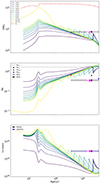 |
Fig. A.1. Evolution of the stellar surface-rotation rate (top panel), stellar Rossby number (middle panel) and X-ray luminosity (bottom panel), under the impact of planetary inward migration. For the stellar initial surface rotation rate we considered the following values Ωin = 1, 2, 3.2, 4, 5, 6, 7, 8, 9, 10, 18 Ω⊙, for the planetary mass Mpl = 1 MJ, and initial planetary orbital distance ain = 0.02 AU. The meaning of the other quantities is the same as in Fig. 3. |
Appendix B: Star with 3 MJ companion and Ωin = 3.2 Ω⊙
In Fig. 7 we show how the host star surface-rotation rate and X-ray luminosity are impacted by the inward migration of a planet with Min = 3 MJ and ain = 0.025 AU, while for the host-star a range of initial surface rotation rates is explored (Ωin = 1, 2, 3.2, 4, 5, 6, 7, 8, 9, 10, 18 Ω⊙). Similarly, in Fig. B.1 we show the results obtained by fixing Ωin to 3.2 Ω⊙ and varying the initial orbital distance in the range ain = 0.02, 0.025, 0.03, 0.035, 0.04, 0.06, 0.08, 0.1 AU. In this context, the shorter the orbital distance and the earlier the engulfment of the planet occurs.
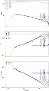 |
Fig. B.1. Evolution of the stellar surface-rotation rate (top panel), stellar Rossby number (middle panel) and X-ray luminosity (bottom panel), under the impact of planetary inward migration. In this case, we fix the initial mass of the planet (3 MJ), the initial surface rotation rate of the host star (Ωin = 3.2 Ω⊙), while we vary the initial orbital distance (ain = 0.02, 0.025, 0.03, 0.035, 0.04, 0.06, 0.08, 0.1 AU). The meaning of the other quantities is the same as in Fig. 3. |
All Tables
All Figures
|
Fig. 1. Hertzsprung-Russell diagram of GJ 504 as obtained from best-fit stellar model (Teff = 6202 K, log(g) = 4.29, R = 1.35 R⊙, L/L⊙ = 2.43) computed with CLES. |
| In the text | |
|
Fig. 2. eROSITA spectra of GJ 504 plotted together with best-fitting apec model and the residuals (both shown in green); see text in Sect. 3.2 and Table 2. |
| In the text | |
|
Fig. 3. Host star’s evolutionary tracks in the SwoP scenario. Top panel: Surface-rotation-rate evolution versus age for our optimal stellar model, with Ωin = 1, 2, 3.2, 4, 5, 6, 7, 8, 9, 10, 18 Ω⊙. The dashed red line shows the evolution of the critical rotation velocity (Ωcrit), defined as the velocity at which the centrifugal acceleration at the equator equals the gravity. The magenta and black markers show GJ 504’s surface rotation rate, with age uncertainties derived from the global and local minimisation modelling, respectively. Middle panel: Evolution of stellar Rossby number (RO). RO for GJ 504 is indicated by the red, black, and blue circles corresponding to the lower, mean, and upper values of the largest age uncertainty, respectively. The grey and black stars represent the values obtained from τconv as in Wright et al. (2011) and Wright et al. (2018). Analogously, the magenta markers represent the same quantities for the smallest age uncertainty. Bottom panel: Evolution of X-ray luminosity for each of the considered rotators. The black and blue markers show the X-ray luminosities from Voges et al. (1999), Wright et al. (2011) (ROSAT) and in this work (eROSITA), respectively. Analogously, the magenta markers represent the same quantities for the smallest age uncertainty. In all panels, the starting point of the tracks corresponds to the dissipation of the protoplanetary disc (2 Myr for Ωin = 18 Ω⊙; 6 Myr for the other ones). |
| In the text | |
|
Fig. 4. Comparison between convective turnover timescale obtained from CLES best-fit model using Eq. (6), and the values computed as in Wright et al. (2011) (grey star) and Wright et al. (2018) (black star). |
| In the text | |
|
Fig. 5. Different orbital evolutions for a planet with 1 ≤ Mplin/MJ ≤ 10 and 0.02 ≤ ain (AU) ≤ 0.1 computed for Ωin = 3.2 Ω⊙ (top panel), Ωin = 5 Ω⊙ (middle panel), and Ωin = 18 Ω⊙ (bottom panel). The salmon-coloured hatched area shows the parameter space for which, after the engulfment, it is possible to reproduce the rotational period and X-ray luminosity of GJ 504 when considering the largest age uncertainty. The lime-hatched area indicates a subset of the salmon-hatched area, for the smaller age uncertainty. The grey shaded area shows the region below the Roche limit. |
| In the text | |
|
Fig. 6. Orbital evolution for 1 MJ planet with 0.02 ≤ ain (AU) ≤ 0.1 and Ωin = 3.2, 18 Ω⊙ (top and bottom panels, respectively). The solid blue lines show the evolution of the orbital distance. The dotted red and dashed black lines indicate the evolution of amin and acor, respectively. The Roche limit is shown by the black dotted line. The cyan and magenta shaded areas represent the extension of the stellar core and envelope along the evolution of the star, respectively. |
| In the text | |
|
Fig. 7. Host star’s evolutionary tracks in the SwP scenario. Evolution of stellar surface-rotation rate (top panel), stellar Rossby number (middle panel), and X-ray luminosity (bottom panel) under the impact of planetary inward migration. For the stellar initial surface-rotation rate, we considered the following values: Ωin = 1, 2, 3.2, 4, 5, 6, 7, 8, 9, 10, 18 Ω⊙. For the planetary mass, we considered Mpl = 3 MJ, and for the initial planetary orbital distance, we considered ain = 0.025 AU. The meaning of the other quantities is the same as in Fig. 3. |
| In the text | |
|
Fig. A.1. Evolution of the stellar surface-rotation rate (top panel), stellar Rossby number (middle panel) and X-ray luminosity (bottom panel), under the impact of planetary inward migration. For the stellar initial surface rotation rate we considered the following values Ωin = 1, 2, 3.2, 4, 5, 6, 7, 8, 9, 10, 18 Ω⊙, for the planetary mass Mpl = 1 MJ, and initial planetary orbital distance ain = 0.02 AU. The meaning of the other quantities is the same as in Fig. 3. |
| In the text | |
|
Fig. B.1. Evolution of the stellar surface-rotation rate (top panel), stellar Rossby number (middle panel) and X-ray luminosity (bottom panel), under the impact of planetary inward migration. In this case, we fix the initial mass of the planet (3 MJ), the initial surface rotation rate of the host star (Ωin = 3.2 Ω⊙), while we vary the initial orbital distance (ain = 0.02, 0.025, 0.03, 0.035, 0.04, 0.06, 0.08, 0.1 AU). The meaning of the other quantities is the same as in Fig. 3. |
| In the text | |
Current usage metrics show cumulative count of Article Views (full-text article views including HTML views, PDF and ePub downloads, according to the available data) and Abstracts Views on Vision4Press platform.
Data correspond to usage on the plateform after 2015. The current usage metrics is available 48-96 hours after online publication and is updated daily on week days.
Initial download of the metrics may take a while.