| Issue |
A&A
Volume 660, April 2022
|
|
|---|---|---|
| Article Number | A144 | |
| Number of page(s) | 7 | |
| Section | The Sun and the Heliosphere | |
| DOI | https://doi.org/10.1051/0004-6361/202142942 | |
| Published online | 29 April 2022 | |
Tracking the 3D evolution of a halo coronal mass ejection using the revised cone model⋆
Key Laboratory of Dark Matter and Space Astronomy, Purple Mountain Observatory, CAS, Nanjing 210023, PR China
e-mail: This email address is being protected from spambots. You need JavaScript enabled to view it.
Received:
17
December
2021
Accepted:
21
February
2022
Abstract
Aims. This paper aims to track the three-dimensional (3D) evolution of a full halo coronal mass ejection (CME) on 2011 June 21.
Methods. The CME results from a nonradial eruption of a filament-carrying flux rope in NOAA active region 11236. The eruption was observed in extreme-ultraviolet (EUV) wavelengths by the extreme-ultraviolet imager (EUVI) on board the ahead and behind Solar TErrestrial RElations Observatory (STEREO) spacecrafts and the atmospheric imaging assembly (AIA) on board the solar dynamics observatory (SDO). The CME was observed by the COR1 coronagraph on board STEREO and the C2 coronagraph on board the large angle spectroscopic coronagraph (LASCO). The revised cone model was slightly modified, with the top of the cone becoming a sphere, which is internally tangent to the legs. Using the multipoint observations, the cone model was applied to derive the morphological and kinematic properties of the CME.
Results. The cone shape fits nicely with the CME observed by EUVI and COR1 on board the STEREO twin spacecraft and LASCO/C2 coronagraph. The cone angle increases sharply from 54° to 130° in the initial phase, indicating a rapid expansion. A relation between the cone angle and the heliocentric distance of the CME leading front is derived, ω = 130° −480d−5, where d is in units of R⊙. The inclination angle decreases gradually from ∼51° to ∼18°, suggesting a trend of radial propagation. The heliocentric distance increases gradually in the initial phase and quickly in the later phase up to ∼11 R⊙. The true speed of the CME reaches ∼1140 km s−1, which is ∼1.6 times higher than the apparent speed in the LASCO/C2 field of view.
Conclusions. The revised cone model is promising in tracking the complete evolution of CMEs.
Key words: Sun: coronal mass ejections (CMEs) / Sun: flares / Sun: filaments, prominences
Movie associated to Fig. 11 is available at https://www.aanda.org
© ESO 2022
1. Introduction
Solar flares (Fletcher et al. 2011) and coronal mass ejections (CMEs; Chen 2011; Patsourakos et al. 2020) are the most powerful activities in the solar atmosphere where a huge mount of magnetic free energy is impulsively released (Aschwanden et al. 2017). A temporal relationship is found between CMEs and the associated flares (Zhang et al. 2001). The initial phase, impulsive acceleration phase, and propagation phase of CMEs are closely related to the preflare phase, rise phase, and decay phase of flares, respectively. It is widely accepted that magnetic flux ropes play an essential role in driving CMEs and flares (Chen & Krall 2003; Aulanier et al. 2010; Zhang et al. 2012, 2022; Cheng et al. 2013; Janvier et al. 2013; Vourlidas et al. 2013; Sahu et al. 2020).
The typical shape of a CME is the well-known three-part structure: a bright core within a dark cavity surrounded by a bright leading front (e.g., Illing & Hundhausen 1985, 1986; Cremades & Bothmer 2004; Veronig et al. 2018; Zhang & Ji 2018; Dai et al. 2021). The frontside halo CMEs, originating near the solar disk center and propagating toward Earth (Howard et al. 1982; Gopalswamy et al. 2007; Byrne et al. 2010; Zhang et al. 2010, 2017; Lu et al. 2017; Yan et al. 2021), may have a severe impact on the solar-terrestrial environment (see Temmer 2021, and references therein). A positive correlation is found between the radial speed and the lateral expansion speed of halo CMEs (Schwenn et al. 2005). The three-dimensional (3D) morphology and kinematics of halo CMEs are critical for an accurate estimation of the arrival time (Shen et al. 2021). Under the assumption that the velocity and angular width keep constant, several versions of cone models were proposed to quickly determine the geometry and kinematics of halo CMEs (e.g., Zhao et al. 2002; Michałek et al. 2003; Xie et al. 2004; Xue et al. 2005; Michalek 2006). Later on, a more sophisticated graduated cylindrical shell (GCS; Thernisien et al. 2006, 2009; Thernisien 2011) model was developed to carry out forward modeling of flux-rope-like CMEs. The GCS model is characterized by the following six geometric parameters: the Carrington longitude (ϕ) and latitude (θ) of the source region, the tilt angle (γ) of the flux rope, the angular width (2α), aspect ratio (κ), and height (h) of the legs, respectively. The model has been successfully applied to track the morphology evolution of CMEs using multi-instrument observations (e.g., Patsourakos et al. 2010a; Temmer et al. 2012, 2021; Cheng et al. 2014; Colaninno & Vourlidas 2015; Cabello et al. 2016; Liu et al. 2018; Gou et al. 2020; O’Kane et al. 2021. To determine the 3D structure of two fronts of a CME, Kwon et al. (2014) put forward a compound model: an ellipsoid model representing the bubble-shaped shock structure (Rouillard et al. 2016) and a GCS model representing the flux rope-shaped structure. Isavnin (2016) created a novel 3D analytic model of CMEs, which is able to reproduce the global shape of a CME with all major deformations. Using the time-dependent, self-similar Gibson-Low model (Gibson & Low 1998), Dai (2022) reconstructed the CME on 2011 March 7 and derived the size, shape, velocity, and magnetic field strength.
To investigate the 3D evolution of CMEs as a result of nonradial filament eruptions, Zhang (2021) proposed a revised cone model (see Fig. 1). The apex of the axisymmetric cone is located at the source region of an eruption instead of the Sun center in the traditional cone models. The model has the following four geometric parameters: the length (r) and angular width (ω) of the cone, an inclination angle (θ1) from the local vertical, and a deviation angle (ϕ1) from the local meridian plane. The model was applied to two partial halo CMEs originating from the western limb on 2011 August 11 and 2012 December 7. The values of θ1 reach up to 70° and 60°. Both CMEs are off-pointed by 30° with respect to the plane of the sky. However, the preliminary application is restricted to the very early evolution of CMEs.
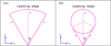 |
Fig. 1. (a) Cross section of the cone in the Yc − Zc plane (Zhang 2021). (b) Cross section of the modified cone in the Yc − Zc plane in this paper. |
On 2011 June 21, a filament-carrying flux rope erupted nonradially from NOAA active region (AR) 11236, giving rise to a C7.7 class long-duration flare and a full halo CME (AW = 360°). Zhou et al. (2017) tracked the 3D evolution of the eruption by using simultaneous observations from the atmospheric imaging assembly (AIA; Lemen et al. 2012) on board the solar dynamics observatory (SDO) and the extreme-ultraviolet imager (EUVI; Wuelser et al. 2004) of the Sun-Earth Connection Coronal and Heliospheric Investigation (SECCHI; Howard et al. 2008) instrument on board the ahead and behind Solar TErrestrial RElations Observatory (STEREO; Kaiser et al. 2008). Guo et al. (2019) obtained a magnetic flux rope before eruption, with the locations of magnetic dips being cospatial with part of the filament and prominence material. Moreover, Guo et al. (2021) performed a data-constrained magnetohydrodynamic (MHD) simulation of the flux rope eruption, which is consistent with the multiperspective observations. For this study, the revised cone model was slightly modified and applied to track the 3D evolution of the halo CME on 2011 June 21. The paper is organized as follows. The method and data analysis are described in Sect. 2. The results are presented in Sect. 3 and compared with previous works in Sect. 4. A brief summary is given in Sect. 5.
2. Method and data analysis
I would like to remind readers of the features of the model (Zhang 2021, see Fig. 1). The Carrington longitude and latitude of the source region of filament eruption are denoted by ϕ2 and β2 (θ2 = 90° −β2), respectively. Hence, the transform between the heliocentric coordinate system (HCS; Xh, Yh, Zh) and local coordinate system (LCS; Xl, Yl, Zl) is as follows1:
 (1)
(1)
where
 (2)
(2)
The transform between the LCS and cone coordinate system (CCS; Xc, Yc, Zc) is performed by a matrix (M1):
 (3)
(3)
where
 (4)
(4)
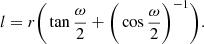
In the revised model, the base of the cone is a sphere section (see model A in Schwenn et al. 2005). The cone has a length of r and an angular width of ω. Therefore, the cross section of the cone is fan-shaped in the Yc − Zc plane, and the leading edge has a total length of l = r (Fig. 1a). In view of the flux rope nature of CMEs in many cases, there is a need to modify the shape of the cone. The top of the cone becomes a sphere, which is internally tangent to the legs (see model C in Schwenn et al. 2005). Figure 1b shows the cross section of the modified cone in the Yc − Zc plane, which is similar to the previous models (e.g., Thernisien et al. 2006). It is obvious that the angular width (ω) is the same, while the total length of the leading edge is as follows:
 (5)
(5)
The aspect ratio (κ) of a CME bubble is defined as the ratio of center height to radius (Patsourakos et al. 2010b; Veronig et al. 2018). In Fig. 1b,  . To determine the geometric parameters of the modified model, observations from multiple viewpoints are required. For the twin satellites of STEREO, the separation angles from the Sun to Earth connection are ϕ0A ≈ 95° for the ahead (STA) and ϕ0B ≈ −92° for the behind (STB) spacecraft on 2011 June 21 (Zhou et al. 2017).
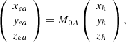
The transform between the STA coordinate system (Xea, Yea, Zea) and HCS is performed by a matrix (M0A):
 (6)
(6)
where
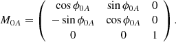 (7)
(7)
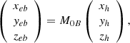
Likewise, the transform between the STB coordinate system (Xeb, Yeb, Zeb) and HCS is performed by a matrix (M0B):
 (8)
(8)
where
 (9)
(9)
The eruptive prominence and associated flare were observed by STA and STB in EUVI 195 Å and 304 Å images with a cadence of 5 min. The S-shaped, filament-carrying flux rope was observed by SDO/AIA in 94 Å (T ≈ 6.3 MK) and 211 Å (T ≈ 2 MK). The associated CME was observed by COR1 coronagraph on board STEREO with a cadence of 5 min and by the C2 coronagraph of the large angle spectroscopic coronagraph (LASCO; Brueckner et al. 1995) instrument on board SOHO2 with a cadence of ≥10 min. The field of views (FOVs) of SECCHI/COR1 and LASCO/C2 are 1.5−4 R⊙ and 2−6 R⊙, respectively. The soft X-ray (SXR) fluxes of the long-duration flare in 0.5−4 Å and 1−8 Å were observed by the GOES spacecraft. The photospheric line-of-sight (LOS) magnetograms before eruption were observed by the helioseismic and magnetic imager (HMI; Scherrer et al. 2012) on board SDO. The global 3D magnetic configuration before eruption was derived from the potential-field source surface (PFSS; Schrijver & De Rosa 2003) modeling.
3. Results
In Fig. 2, the top panel shows the SXR light curves of the flare. The SXR flux in 1−8 Å increases from ∼01:18 UT to the peak value at ∼03:26 UT before decreasing gradually. During the impulsive phase, the constructed flux rope (green diamonds) rises quickly from ∼02:00 UT until ∼02:48 UT (Guo et al. 2021).
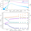 |
Fig. 2. (a) SXR light curves of the flare in 1–8 Å (magenta line) and 0.5–4 Å (blue line). The yellow dashed lines represent the start (∼01:18 UT) and peak (∼03:26 UT) times of the flare. The green diamonds denote the heights of magnetic flux rope in the MHD simulation (Guo et al. 2021). (b–d) Time evolutions of the real distance (d) of the CME leading edge, angular width (ω), aspect ratio (κ), and inclination angle (θ1) of the cone. Panel b: the heights of the CME in the LASCO/C2 FOV are drawn with brown triangles. |
In Fig. 3, the top panels show the bright prominence observed by STEREO/EUVI in 304 Å and the sigmoid observed by SDO/AIA in 94 Å before eruption (Zhou et al. 2017). The middle panels show the CME bubble observed by EUVI in 195 Å (base difference) and the sigmoid in 94 Å during eruption. The bottom panels show the hot and bright post-flare loops (PFLs) after eruption.
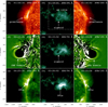 |
Fig. 3. Prominence observed by STA (a) and STB (c) in 304 Å before eruption. The CME bubble observed by STA (d) and STB (f) in 195 Å base-difference images during eruption. Post-flare loops (PFLs) observed by STA (g) and STB (i) in 195 Å after eruption. The AIA 94 Å images feature the sigmoid before (b) and during (e) eruption, and the PFLs (h). The white dashed box in panel b signifies the FOV of Fig. 4a. |
In Fig. 4, the left panel shows the LOS magnetogram of AR 11236 at 01:02:56 UT, with the locations of sigmoid being superposed with cyan crosses. The sigmoid is roughly along the polarity inversion line. The right panel shows the large-scale 3D magnetic configuration around the AR at 00:04 UT using PFSS modeling. The orange arrow indicates the projected direction of filament eruption. It is revealed that the AR is adjacent to open field lines (magenta) which may deflect the eruption in longitude (Cremades et al. 2006; Kilpua et al. 2009; Panasenco et al. 2013; Yang et al. 2018).
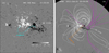 |
Fig. 4. (a) LOS magnetogram of AR 11236 at 01:02:56 UT. The cyan crosses represent the locations of sigmoid in 94 Å. (b) Large-scale 3D magnetic configuration around the AR at 00:04 UT derived from PFSS modeling. The white and magenta lines represent the closed and open field lines. The orange arrow indicates the projected direction of the filament eruption. |
In Fig. 5, base-difference images in 195 Å observed by STA and STB at 02:10 UT are displayed in panels a and c, respectively. The CME bubble with enhanced intensity is pointed out by arrows. The base-difference image in 211 Å observed by AIA at 02:10 UT is displayed in panel b, where the projected CME leading edge is blurred and incoherent. Therefore, the reconstruction of the cone was performed using the simultaneous base-difference images of STEREO. In the bottom panels, the projections of the reconstructed cone are superposed with magenta dots. It is obvious that the slightly modified cone (Fig. 1b) can nicely fit the CME bubble (see panels d and f). The parameters of r, ω, θ1, and the corresponding l (Eq. (5)) are listed in Table 1. The deviation angle ϕ1 = −45° was derived from the data-constrained MHD simulation (Guo et al. 2021) and keeps constant for convenience. The initial eruption of flux rope is inclining southward from the radial direction by ∼51° and the length of CME bubble is ∼555″. To estimate the errors in the derived best-fit cone for a sample snapshot, each parameter was changed a few times while keeping all the others equal to their best-fit values. The tolerated offsets from the best-fit cone parameters are considered as uncertainties.
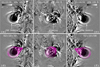 |
Fig. 5. Top panels: base-difference images in 195 Å observed by STA/EUVI (a) and STB/EUVI (c) at 02:10 UT. Base-difference image in 211 Å observed by SDO/AIA at 02:10 UT (b). The arrows point to the CME bubble and dimming. Bottom panels: same images as the top panels, with the projections of the reconstructed cone being superposed (magenta dots). |
Parameters of the cones at different times.
The EUV difference images and projected cones at 02:15 UT, 02:20 UT, and 02:25 UT are displayed in Figs. 6–8, respectively. It is clear that the cone in Fig. 1b can still fit the CME bubbles within the EUVI FOV. In the AIA FOV, the projected cones cover most of the corresponding dimming regions on the disk. The derived parameters are listed in Table 1. The cone angle (ω) increases from ∼54° to ∼76° within 15 min at a rate of ∼1.5° min−1, indicating a rapidly lateral expansion. The inclination angle (θ1) decreases from ∼51° to ∼44° at the same time, suggesting a tendency for radial propagation. The length of the leading edge (l) increases gradually from 555″ to 769″. The heliocentric distance (d) of the leading edge increases from ∼1.44 R⊙ to ∼1.68 R⊙ accordingly (see Figs. 2b–d). It is noted that CMEs and EUV waves are frequently related (Chen 2011).
During 02:30−03:10 UT, the CME leading edge escaped the STEREO/EUVI FOV and entered the STEREO/COR1 FOV. However, the CME does not appear in the LASCO/C2 FOV until 03:16 UT. Figure 9 shows selected base-difference images of the CME observed by COR1 during 02:30−03:10 UT. The projections of reconstructed cones are superposed with magenta dots. The parameters of the cone are listed in Table 1. The cone angle increases gradually from ∼110° to ∼130° within half an hour and reaches a plateau. The inclination angle decreases from ∼36° to ∼18° in the meantime. The total length of the leading edge increase quickly from ∼793″ to ∼2729″, and the corresponding heliocentric distance increases from ∼1.75 R⊙ to ∼3.86 R⊙ (see Figs. 2b–d).
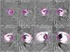 |
Fig. 9. Selected base-difference images of the CME observed by STEREO/COR1 during 02:30−03:10 UT. The projections of reconstructed cones are superposed with magenta dots. |
After 03:15 UT, the CME leading edge escapes the COR1 FOV and enters the C2 FOV. Consequently, there is no constraint of the cone from STEREO observations anymore. Assuming that the CME shape remains self-similar and the direction keeps constant in the LASCO FOV, the cone angle is set to be 130° and the inclination angle is set to be 18° (see Table 1). In Fig. 10, the top panels show base-difference images of the CME observed by LASCO/C2 during 03:16−04:00 UT. In the bottom panels, the projections of reconstructed cones are superposed with magenta dots, which could moderately cover most of the CME. The length of the cone increases from ∼5400″ to ∼9500″, and the corresponding heliocentric distance increases from ∼6.7 R⊙ to ∼11.0 R⊙ (see Figs. 2b–d). The real speed of the CME leading edge was calculated to be ∼1139 km s−1. In Fig. 2b, the heights of the CME in the LASCO/C2 FOV are drawn with brown triangles, with an apparent linear speed of ∼724 km s−1. Hence, the ratio of real speed to the apparent speed of the CME is ∼1.6. Such a high speed for the CME is likely to drive a shock wave (Ontiveros & Vourlidas 2009). In Fig. 10, the CME leading front might be blended with the shock front, which makes it difficult to distinguish the CME front. In Fig. 2b, the leap of the heliocentric distance at 03:16 UT is probably caused by an overestimation of CME height when constraint from another viewpoint is unavailable. However, a type II radio burst accompanying the shock wave is absent in the radio dynamic spectra during the eruption. An in-depth investigation is needed to address this issue (Rouillard et al. 2012).
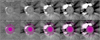 |
Fig. 10. Top panels: base-difference images of the CME observed by LASCO/C2 during 03:16−04:00 UT. Bottom panels: same difference images with projections of reconstructed cones being superposed with magenta dots. |
Figure 11 shows snapshots of the Sun (yellow dots) and reconstructed CME cones from viewpoints of STA (magenta dots), STB (magenta dots), SDO (green dots), and north pole (purple dots), respectively. The whole evolution during 02:10−04:00 UT is demonstrated in an online animation (cones.mp4). The nonradial eruption of the prominence-carrying flux rope is like blowing a bubble. The time variations of ω, θ1, and d are plotted in Fig. 2. The cone angle increases sharply during 02:10−02:40 UT, which is coincident with the fast rise of the flux rope (Fig. 2a), indicating a rapid expansion and propagation in the initial phase. Patsourakos et al. (2010b) studied the early evolution of the eruptive flare on 2010 June 13. A short-lived, lateral overexpansion with a declining aspect ratio was discovered in the deceleration phase. Veronig et al. (2018) investigated the genesis of an extremely fast CME on 2017 September 10, finding that the strong lateral overexpansion of the CME bubble drives the fast-mode EUV (shock) wave during the impulsive phase of the related X8.2 class flare. In the current case, the aspect ratio declines from ∼2.2 at 02:10 UT to ∼1.1 at 02:55 UT, which is accordant with the lateral expansion of the CME bubble (Fig. 2c). The heliocentric distance of the CME leading front increases gradually in the initial phase and quickly in the later phase up to ∼11 R⊙.
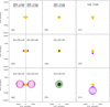 |
Fig. 11. Snapshots of the Sun (yellow dots) and reconstructed CME cones from viewpoints of STA (magenta dots), STB (magenta dots), SDO (green dots), and north pole (purple dots). An animation (cones.mp4) is available online. |
4. Discussion
Since CMEs are the most spectacular driver of space weather on Earth, the morphology, propagation, and kinematics of CMEs are crucial to an accurate prediction of space weather. The 3D reconstructions of CMEs using multipoint observations are substantial (e.g., Moran & Davila 2004; Byrne et al. 2010; Feng et al. 2012; Rouillard et al. 2016). Byrne et al. (2010) used an elliptical tie-pointing technique to reconstruct a full CME front in 3D. The angular width increases with the heliocentric distance from 2 R⊙ to 46 R⊙ with a power law form. The deflection from the radial from the onset decreases with distance as well, suggesting an equatorward deflection. Shen et al. (2011) investigated the kinematic evolution of the CME on 2007 October 8. The CME first deflected to the lower latitude by ∼30° and then propagated radially. Gui et al. (2011) analyzed the deflections of ten CMEs observed by the STEREO twin spacecraft and concluded that the deflections are primarily controlled by the background magnetic field. Isavnin et al. (2014) explored the whole propagations of 14 CMEs from the Sun to 1 AU, finding that the deflection of flux ropes occurs below 30 R⊙ in most cases. Zhang (2021) applied the revised cone model to two CMEs as a result of nonradial prominence eruptions. Similarly, the inclination angles are 60° −70° at the very beginning, and the directions of CMEs become radial in the LASCO FOV. In the current event, the halo CME experiences lateral expansion during its eruption. A crude fitting between ω and d results in a relationship of ω = 130° −480d−5, where d is in units of R⊙. The inclination angle (θ1) decreases from ∼51° to ∼18°, suggesting a trend of radial propagation. A crude fitting between θ1 and d results in a relationship of θ1 = 81.7° −23.45d, where 1.4 R⊙ ≤d ≤ 3.0 R⊙.
Compared with the preliminary application in Zhang (2021), the reconstructions of the CME extend to the LASCO/C2 FOV, which is a step forward. It should be emphasized that the performance still has limitations. Firstly, the deviation angle (ϕ1) is assumed to keep constant for simplicity. In addition, the angular width and direction of the CME are assumed to keep constant in the LASCO/C2 FOV, since the leading edge has escaped the COR1 FOV. The not exactly satisfactory fitting of the C2 data might not only arise from the possible confusion with the shock wave, but due to the fact that the model is applied to a single viewpoint as well. Secondly, the time cadence of LASCO/C2 is ≥10 min, which is two times lower than EUVI and COR1. Finally, considering the dispersed shape and weak intensity of the CME in the LASCO/C3 FOV, the reconstruction was not performed after 04:00 UT.
In the future, comprehensive tracking of the CME propagation is feasible in combination with the GCS modeling (Thernisien et al. 2006). The revised cone model will be applied to a 3D reconstruction of CMEs observed by the Lyman-α Solar Telescope (LST; Feng et al. 2019; Li et al. 2019) on board the advanced space-based solar observatory (ASO-S; Gan et al. 2019), the Metis (Antonucci et al. 2020) and Heliospheric Imager (SoloHI; Howard et al. 2020) on board solar orbiter (Müller et al. 2020). The model is also valuable in studying fast CMEs driving shock waves, with additional constraints from radio observations (e.g., Gopalswamy et al. 2009; Zucca et al. 2018; Mancuso et al. 2019). The reconstructed morphology and direction of a CME may serve as the initial condition for MHD numerical simulations (Shen et al. 2021; Yang et al. 2021).
5. Summary
In this paper, the revised cone model is slightly modified and applied to a full halo CME as a result of nonradial flux rope eruption on 2011 June 21. The main results are as follows:
-
The cone shape fits well with the CME observed by EUVI and COR1 on board the STEREO twin spacecraft and LASCO/C2 coronagraph.
-
The cone angle increases sharply from ∼54° to ∼130° in the initial phase, indicating a rapid expansion. A relation between the cone angle and heliocentric distance of the CME leading front is derived, ω = 130° −480d−5, where d is in units of R⊙. The inclination angle decreases gradually from ∼51° to ∼18°, suggesting a trend of radial propagation. The heliocentric distance increases gradually in the initial phase and quickly in the later phase up to ∼11 R⊙. The true speed of the CME reaches ∼1140 km s−1, which is ∼1.6 times higher than the apparent speed in the LASCO/C2 FOV.
-
The revised cone model is promising in tracking the complete evolution of CMEs and will contribute to the space weather forecast.
Movies
Movie 1 associated with Fig. 11 (cones) Access Supplementary Material
There is an unintended error in Eq. (1) of Zhang (2021).
Acknowledgments
The author appreciates the reviewer for valuable suggestions to improve the quality of this article. The author is also grateful to Drs. Y. Guo and Z. J. Zhou for helpful discussions. SDO is a mission of NASA’s Living With a Star Program. AIA data are courtesy of the NASA/SDO science teams. STEREO/SECCHI data are provided by a consortium of US, UK, Germany, Belgium, and France. This work is funded by the National Key R&D Program of China 2021YFA1600500 (2021YFA1600502), NSFC grants (Nos. 11773079, 11790302), and the Strategic Priority Research Program on Space Science, CAS (XDA15052200, XDA15320301).
References
- Antonucci, E., Romoli, M., Andretta, V., et al. 2020, A&A, 642, A10 [NASA ADS] [CrossRef] [EDP Sciences] [Google Scholar]
- Aschwanden, M. J., Caspi, A., Cohen, C. M. S., et al. 2017, ApJ, 836, 17 [Google Scholar]
- Aulanier, G., Török, T., Démoulin, P., et al. 2010, ApJ, 708, 314 [CrossRef] [Google Scholar]
- Brueckner, G. E., Howard, R. A., Koomen, M. J., et al. 1995, Sol. Phys., 162, 357 [NASA ADS] [CrossRef] [Google Scholar]
- Byrne, J. P., Maloney, S. A., McAteer, R. T. J., et al. 2010, Nat. Commun., 1, 74 [NASA ADS] [CrossRef] [Google Scholar]
- Cabello, I., Cremades, H., Balmaceda, L., et al. 2016, Sol. Phys., 291, 1799 [NASA ADS] [CrossRef] [Google Scholar]
- Chen, P. F. 2011, Liv. Rev. Sol. Phys., 8, 1 [Google Scholar]
- Chen, J., & Krall, J. 2003, J. Geophys. Res. (Space Phys.), 108, 1410 [NASA ADS] [CrossRef] [Google Scholar]
- Cheng, X., Zhang, J., Ding, M. D., et al. 2013, ApJ, 763, 43 [NASA ADS] [CrossRef] [Google Scholar]
- Cheng, X., Ding, M. D., Guo, Y., et al. 2014, ApJ, 780, 28 [Google Scholar]
- Colaninno, R. C., & Vourlidas, A. 2015, ApJ, 815, 70 [Google Scholar]
- Cremades, H., & Bothmer, V. 2004, A&A, 422, 307 [NASA ADS] [CrossRef] [EDP Sciences] [Google Scholar]
- Cremades, H., Bothmer, V., & Tripathi, D. 2006, Adv. Space Res., 38, 461 [NASA ADS] [CrossRef] [Google Scholar]
- Dai, X. 2022, ApJ, 925, 24 [NASA ADS] [CrossRef] [Google Scholar]
- Dai, J., Zhang, Q., Zhang, Y., et al. 2021, ApJ, 923, 74 [NASA ADS] [CrossRef] [Google Scholar]
- Feng, L., Inhester, B., Wei, Y., et al. 2012, ApJ, 751, 18 [Google Scholar]
- Feng, L., Li, H., Chen, B., et al. 2019, Res. Astron. Astrophys., 19, 162 [CrossRef] [Google Scholar]
- Fletcher, L., Dennis, B. R., Hudson, H. S., et al. 2011, Space Sci. Rev., 159, 19 [Google Scholar]
- Gan, W.-Q., Zhu, C., Deng, Y.-Y., et al. 2019, Res. Astron. Astrophys., 19, 156 [Google Scholar]
- Gibson, S. E., & Low, B. C. 1998, ApJ, 493, 460 [NASA ADS] [CrossRef] [Google Scholar]
- Gopalswamy, N., Yashiro, S., & Akiyama, S. 2007, J. Geophys. Res. (Space Phys.), 112, A06112 [Google Scholar]
- Gopalswamy, N., Thompson, W. T., Davila, J. M., et al. 2009, Sol. Phys., 259, 227 [NASA ADS] [CrossRef] [Google Scholar]
- Gou, T., Veronig, A. M., Liu, R., et al. 2020, ApJ, 897, L36 [NASA ADS] [CrossRef] [Google Scholar]
- Gui, B., Shen, C., Wang, Y., et al. 2011, Sol. Phys., 271, 111 [NASA ADS] [CrossRef] [Google Scholar]
- Guo, Y., Xu, Y., Ding, M. D., et al. 2019, ApJ, 884, L1 [NASA ADS] [CrossRef] [Google Scholar]
- Guo, Y., Zhong, Z., Ding, M. D., et al. 2021, ApJ, 919, 39 [NASA ADS] [CrossRef] [Google Scholar]
- Howard, R. A., Michels, D. J., Sheeley, N. R., et al. 1982, ApJ, 263, L101 [NASA ADS] [CrossRef] [Google Scholar]
- Howard, R. A., Moses, J. D., Vourlidas, A., et al. 2008, Space Sci. Rev., 136, 67 [NASA ADS] [CrossRef] [Google Scholar]
- Howard, R. A., Vourlidas, A., Colaninno, R. C., et al. 2020, A&A, 642, A13 [NASA ADS] [CrossRef] [EDP Sciences] [Google Scholar]
- Illing, R. M. E., & Hundhausen, A. J. 1985, J. Geophys. Res., 90, 275 [Google Scholar]
- Illing, R. M. E., & Hundhausen, A. J. 1986, J. Geophys. Res., 91, 10951 [Google Scholar]
- Isavnin, A. 2016, ApJ, 833, 267 [Google Scholar]
- Isavnin, A., Vourlidas, A., & Kilpua, E. K. J. 2014, Sol. Phys., 289, 2141 [NASA ADS] [CrossRef] [Google Scholar]
- Janvier, M., Aulanier, G., Pariat, E., et al. 2013, A&A, 555, A77 [NASA ADS] [CrossRef] [EDP Sciences] [Google Scholar]
- Kaiser, M. L., Kucera, T. A., Davila, J. M., et al. 2008, Space Sci. Rev., 136, 5 [Google Scholar]
- Kilpua, E. K. J., Pomoell, J., Vourlidas, A., et al. 2009, Ann. Geophys., 27, 4491 [NASA ADS] [CrossRef] [Google Scholar]
- Kwon, R.-Y., Zhang, J., & Olmedo, O. 2014, ApJ, 794, 148 [NASA ADS] [CrossRef] [Google Scholar]
- Lemen, J. R., Title, A. M., Akin, D. J., et al. 2012, Sol. Phys., 275, 17 [Google Scholar]
- Li, H., Chen, B., Feng, L., et al. 2019, Res. Astron. Astrophys., 19, 158 [Google Scholar]
- Liu, Y. A., Liu, Y. D., Hu, H., et al. 2018, ApJ, 854, 126 [NASA ADS] [CrossRef] [Google Scholar]
- Lu, L., Inhester, B., Feng, L., et al. 2017, ApJ, 835, 188 [NASA ADS] [CrossRef] [Google Scholar]
- Mancuso, S., Frassati, F., Bemporad, A., et al. 2019, A&A, 624, L2 [NASA ADS] [CrossRef] [EDP Sciences] [Google Scholar]
- Michalek, G. 2006, Sol. Phys., 237, 101 [NASA ADS] [CrossRef] [Google Scholar]
- Michałek, G., Gopalswamy, N., & Yashiro, S. 2003, ApJ, 584, 472 [Google Scholar]
- Moran, T. G., & Davila, J. M. 2004, Science, 305, 66 [Google Scholar]
- Müller, D., St. Cyr, O.C., & Zouganelis, I., et al. 2020, A&A, 642, A1 [NASA ADS] [CrossRef] [EDP Sciences] [Google Scholar]
- O’Kane, J., Green, L. M., Davies, E. E., et al. 2021, A&A, 656, L6 [NASA ADS] [CrossRef] [EDP Sciences] [Google Scholar]
- Ontiveros, V., & Vourlidas, A. 2009, ApJ, 693, 267 [NASA ADS] [CrossRef] [Google Scholar]
- Panasenco, O., Martin, S. F., Velli, M., et al. 2013, Sol. Phys., 287, 391 [NASA ADS] [CrossRef] [Google Scholar]
- Patsourakos, S., Vourlidas, A., & Kliem, B. 2010a, A&A, 522, A100 [NASA ADS] [CrossRef] [EDP Sciences] [Google Scholar]
- Patsourakos, S., Vourlidas, A., & Stenborg, G. 2010b, ApJ, 724, L188 [NASA ADS] [CrossRef] [Google Scholar]
- Patsourakos, S., Vourlidas, A., Török, T., et al. 2020, Space Sci. Rev., 216, 131 [Google Scholar]
- Rouillard, A. P., Sheeley, N. R., Tylka, A., et al. 2012, ApJ, 752, 44 [CrossRef] [Google Scholar]
- Rouillard, A. P., Plotnikov, I., Pinto, R. F., et al. 2016, ApJ, 833, 45 [NASA ADS] [CrossRef] [Google Scholar]
- Sahu, S., Joshi, B., Mitra, P. K., et al. 2020, ApJ, 897, 157 [NASA ADS] [CrossRef] [Google Scholar]
- Scherrer, P. H., Schou, J., Bush, R. I., et al. 2012, Sol. Phys., 275, 207 [Google Scholar]
- Schrijver, C. J., & De Rosa, M. L. 2003, Sol. Phys., 212, 165 [Google Scholar]
- Schwenn, R., dal Lago, A., Huttunen, E., et al. 2005, Ann. Geophys., 23, 1033 [NASA ADS] [CrossRef] [Google Scholar]
- Shen, C., Wang, Y., Gui, B., et al. 2011, Sol. Phys., 269, 389 [NASA ADS] [CrossRef] [Google Scholar]
- Shen, F., Liu, Y., & Yang, Y. 2021, ApJS, 253, 12 [NASA ADS] [CrossRef] [Google Scholar]
- Temmer, M. 2021, Liv. Rev. Sol. Phys., 18, 4 [NASA ADS] [CrossRef] [Google Scholar]
- Temmer, M., Vršnak, B., Rollett, T., et al. 2012, ApJ, 749, 57 [NASA ADS] [CrossRef] [Google Scholar]
- Temmer, M., Holzknecht, L., Dumbović, M., et al. 2021, J. Geophys. Res. (Space Phys.), 126, e28380 [NASA ADS] [Google Scholar]
- Thernisien, A. 2011, ApJS, 194, 33 [Google Scholar]
- Thernisien, A. F. R., Howard, R. A., & Vourlidas, A. 2006, ApJ, 652, 763 [Google Scholar]
- Thernisien, A., Vourlidas, A., & Howard, R. A. 2009, Sol. Phys., 256, 111 [Google Scholar]
- Veronig, A. M., Podladchikova, T., Dissauer, K., et al. 2018, ApJ, 868, 107 [NASA ADS] [CrossRef] [Google Scholar]
- Vourlidas, A., Lynch, B. J., Howard, R. A., et al. 2013, Sol. Phys., 284, 179 [NASA ADS] [Google Scholar]
- Wuelser, J.-P., Lemen, J. R., Tarbell, T. D., et al. 2004, Proc. SPIE, 5171, 111 [Google Scholar]
- Xie, H., Ofman, L., & Lawrence, G. 2004, J. Geophys. Res. (Space Phys.), 109, A03109 [NASA ADS] [Google Scholar]
- Xue, X. H., Wang, C. B., & Dou, X. K. 2005, J. Geophys. Res. (Space Phys.), 110, A08103 [NASA ADS] [CrossRef] [Google Scholar]
- Yan, X., Wang, J., Guo, Q., et al. 2021, ApJ, 919, 34 [NASA ADS] [CrossRef] [Google Scholar]
- Yang, J., Dai, J., Chen, H., et al. 2018, ApJ, 862, 86 [CrossRef] [Google Scholar]
- Yang, L., Wang, H., Feng, X., et al. 2021, ApJ, 918, 31 [NASA ADS] [CrossRef] [Google Scholar]
- Zhang, Q. M. 2021, A&A, 653, L2 [NASA ADS] [CrossRef] [EDP Sciences] [Google Scholar]
- Zhang, Q. M., & Ji, H. S. 2018, ApJ, 860, 113 [NASA ADS] [CrossRef] [Google Scholar]
- Zhang, J., Dere, K. P., Howard, R. A., et al. 2001, ApJ, 559, 452 [Google Scholar]
- Zhang, Q.-M., Guo, Y., Chen, P.-F., et al. 2010, Res. Astron. Astrophys., 10, 461 [Google Scholar]
- Zhang, J., Cheng, X., & Ding, M.-D. 2012, Nat. Commun., 3, 747 [Google Scholar]
- Zhang, Q. M., Su, Y. N., & Ji, H. S. 2017, A&A, 598, A3 [NASA ADS] [CrossRef] [EDP Sciences] [Google Scholar]
- Zhang, Q. M., Chen, J. L., Li, S. T., et al. 2022, Sol. Phys., 297, 18 [NASA ADS] [CrossRef] [Google Scholar]
- Zhao, X. P., Plunkett, S. P., & Liu, W. 2002, J. Geophys. Res. (Space Phys.), 107, 1223 [NASA ADS] [CrossRef] [Google Scholar]
- Zhou, Z., Zhang, J., Wang, Y., et al. 2017, ApJ, 851, 133 [NASA ADS] [CrossRef] [Google Scholar]
- Zucca, P., Morosan, D. E., Rouillard, A. P., et al. 2018, A&A, 615, A89 [NASA ADS] [CrossRef] [EDP Sciences] [Google Scholar]
All Tables
All Figures
|
Fig. 1. (a) Cross section of the cone in the Yc − Zc plane (Zhang 2021). (b) Cross section of the modified cone in the Yc − Zc plane in this paper. |
| In the text | |
|
Fig. 2. (a) SXR light curves of the flare in 1–8 Å (magenta line) and 0.5–4 Å (blue line). The yellow dashed lines represent the start (∼01:18 UT) and peak (∼03:26 UT) times of the flare. The green diamonds denote the heights of magnetic flux rope in the MHD simulation (Guo et al. 2021). (b–d) Time evolutions of the real distance (d) of the CME leading edge, angular width (ω), aspect ratio (κ), and inclination angle (θ1) of the cone. Panel b: the heights of the CME in the LASCO/C2 FOV are drawn with brown triangles. |
| In the text | |
|
Fig. 3. Prominence observed by STA (a) and STB (c) in 304 Å before eruption. The CME bubble observed by STA (d) and STB (f) in 195 Å base-difference images during eruption. Post-flare loops (PFLs) observed by STA (g) and STB (i) in 195 Å after eruption. The AIA 94 Å images feature the sigmoid before (b) and during (e) eruption, and the PFLs (h). The white dashed box in panel b signifies the FOV of Fig. 4a. |
| In the text | |
|
Fig. 4. (a) LOS magnetogram of AR 11236 at 01:02:56 UT. The cyan crosses represent the locations of sigmoid in 94 Å. (b) Large-scale 3D magnetic configuration around the AR at 00:04 UT derived from PFSS modeling. The white and magenta lines represent the closed and open field lines. The orange arrow indicates the projected direction of the filament eruption. |
| In the text | |
|
Fig. 5. Top panels: base-difference images in 195 Å observed by STA/EUVI (a) and STB/EUVI (c) at 02:10 UT. Base-difference image in 211 Å observed by SDO/AIA at 02:10 UT (b). The arrows point to the CME bubble and dimming. Bottom panels: same images as the top panels, with the projections of the reconstructed cone being superposed (magenta dots). |
| In the text | |
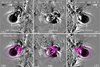 |
Fig. 6. Same as Fig. 5, but for images at 02:15 UT. |
| In the text | |
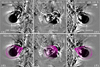 |
Fig. 7. Same as Fig. 5, but for images at 02:20 UT. |
| In the text | |
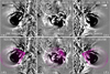 |
Fig. 8. Same as Fig. 5, but for images at 02:25 UT. |
| In the text | |
|
Fig. 9. Selected base-difference images of the CME observed by STEREO/COR1 during 02:30−03:10 UT. The projections of reconstructed cones are superposed with magenta dots. |
| In the text | |
|
Fig. 10. Top panels: base-difference images of the CME observed by LASCO/C2 during 03:16−04:00 UT. Bottom panels: same difference images with projections of reconstructed cones being superposed with magenta dots. |
| In the text | |
|
Fig. 11. Snapshots of the Sun (yellow dots) and reconstructed CME cones from viewpoints of STA (magenta dots), STB (magenta dots), SDO (green dots), and north pole (purple dots). An animation (cones.mp4) is available online. |
| In the text | |
Current usage metrics show cumulative count of Article Views (full-text article views including HTML views, PDF and ePub downloads, according to the available data) and Abstracts Views on Vision4Press platform.
Data correspond to usage on the plateform after 2015. The current usage metrics is available 48-96 hours after online publication and is updated daily on week days.
Initial download of the metrics may take a while.