| Issue |
A&A
Volume 660, April 2022
|
|
|---|---|---|
| Article Number | A50 | |
| Number of page(s) | 9 | |
| Section | The Sun and the Heliosphere | |
| DOI | https://doi.org/10.1051/0004-6361/202142328 | |
| Published online | 08 April 2022 | |
Reconstruction of the magnetic connection from Mercury to the solar corona during enhancements in the solar proton fluxes at Mercury
1
ASI – Italian Space Agency, Via del Politecnico snc, 00133 Rome, Italy
2
INGV, Via di Vigna Murata 605, 00133 Rome, Italy
e-mail: This email address is being protected from spambots. You need JavaScript enabled to view it.
3
Dipartimento di Fisica, Università della Calabria, Arcavacata di Rende, CS, Italy
4
INAF-IAPS, Via del Fosso del Cavaliere, Rome, Italy
Received:
29
September
2021
Accepted:
7
January
2022
Abstract
Aims. We study the magnetic connection between Mercury and the solar corona based on energetic proton events measured near Mercury by MESSENGER during 2011−2013 in order to identify the possible source of the accelerated particles on the solar surface.
Methods. The transport of the magnetic field lines in the heliosphere was evaluated with a Monte Carlo code that gives a random displacement at each step of the integration along the Parker magnetic field model. The simulation was tailored to each specific event by using the magnetic fluctuation levels obtained at Mercury by MESSENGER and the values of the solar wind velocity measured at 1 AU by the Advanced Composition Explorer satellite. We selected seven case studies for which an increase in the proton fluxes of at least two orders of magnitude with respect to the background level was observed. For each selected case, we took the background magnetic field map (magnetogram) at the source surface of the solar wind (r = 2.5 R⊙) into account. By considering the relative position of Mercury and the Earth on the day on which the enhancement in the proton fluxes was observed by MESSENGER, we obtained the position of the active regions on the solar surface as seen by Mercury.
Results. The footpoint of the Parker spiral passing Mercury was reconstructed for all of the selected events. By considering the values of the fluctuation levels of the interplanetary magnetic field recorded by MAG-MESSENGER two days before the event and the values of the fluctuation levels of the interplanetary magnetic field on the day on which the event was observed, we are also able to appreciate the effects on the solar wind magnetic field perturbations induced by the shock of the coronal mass ejection. This technique will also be useful for the interpretation of energetic particle observations by BepiColombo.
Key words: Sun: particle emission / Sun: coronal mass ejections (CMEs) / methods: numerical / planet-star interactions / turbulence
© A. Ippolito et al. 2022
 Open Access article, published by EDP Sciences, under the terms of the Creative Commons Attribution License (https://creativecommons.org/licenses/by/4.0), which permits unrestricted use, distribution, and reproduction in any medium, provided the original work is properly cited.
1. Introduction
The close proximity of Mercury to the Sun and its weak internal magnetic field create the conditions for a strong planetary response to the extreme solar wind properties and intense solar energetic particle (SEP) fluxes. During large SEP events, a significant portion of the high-energy particles will have direct access to the closed-field-line inner magnetosphere (Leblanc et al. 2003; Gershman et al. 2015). The interaction of SEPs with Mercury’s surface can create a variety of secondary products, including neutrals, photons, and secondary charged particles that interact with Mercury’s exosphere and contribute to magnetospheric plasma mass loading (Milillo et al. 2021). For this reason, understanding the source at the solar surface of the events occurring at Mercury is important to understand the general interaction of Mercury and the Sun in an evolutive view as well.
Solar energetic particles are generated under two main conditions: in shock waves driven by coronal mass ejections (CMEs), and in strong solar flares. The SEP characteristics are quite variable and are classified into two general groups. The first SEPs are gradual and wide, and the second SEPs are impulsive and sharp (Reames 2013). In both cases, solar corona and/or solar wind ions are accelerated up to energies of 10 MeV−1 GeV. Existing models, such as the ensemble WSA-ENLIL+Cone model from the Community Coordinated Modeling Center (CCMC), simulate the propagation of a CME in the vicinity of a planet (Odstricil 2003; Plainaki et al. 2016; Dewey et al. 2015). Based on the WSA coronal model (Arge & Pizzo 2000; Arge et al. 2004), the global 3D magnetohydrodynamic (MHD) ENLIL model provides the time-dependent description of the background solar wind plasma and magnetic field. In this model, a homogeneous, overpressure hydrodynamic plasma cloud is launched through the inner boundary of the heliospheric computational domain and into the background solar wind. The CME cloud is modeled as a sphere, although other CME shapes are supported by the model; furthermore, the outer radial boundary can be adjusted to include planets in order to study the arrival time and the induced effects in the vicinity of the planet. A further model to reconstruct a three-dimensional tomography of interplanetary disturbances has been developed at the University of California, San Diego (Jackson & Hick 2004). This consists of a computer-assisted tomography (CAT) program that modifies a three-dimensional kinematic heliospheric model to fit interplanetary scintillation (IPS) or Thomson-scattering observations. The tomography program iteratively changes this global model to perform a least-squares fit of the data. Additional information about the arrival of SEPs can be obtained by studying the particle propagation as described below. These particles propagate along the magnetic field lines of the solar wind, where significant levels of magnetic turbulence are found. Therefore, the bundle of solar wind magnetic field lines intersecting Mercury’s magnetosphere does not simply follow the Parker spiral, but spreads out in space because of irregularities in the magnetic field (Belcher & Davis 1971; Bavassano et al. 1982). Low-frequency magnetic fluctuations induce a random displacement of magnetic field lines that can be viewed as a magnetic field line diffusion (Jokipii & Parker 1968; Zimbardo et al. 2000; Pommois et al. 2001; Pucci et al. 2016). If the Larmor radius of charged particles is much smaller than the typical turbulence scale lengths, with good approximation, they move along the magnetic field lines so that the magnetic field structure determines particle transport. As a consequence, energetic particles propagate not only along the average magnetic field, but also transverse to it, and the magnetic connection between two points depends on the features of the magnetic turbulence. Tracking the magnetic field line back to its footpoint in the solar corona will lead to an (uncertainty) area whose extent is proportional to the level of magnetic turbulence. An interesting study conducted by Winslow et al. (2015) of the occurrence of CMEs at Mercury constitutes a solid base from which to proceed in the investigation of the energetic particle transport at Mercury, and to check our understanding of the complex phenomena involved: Starting from their CME catalog, we applied the method developed by Ippolito et al. (2005) in order to study the relation between flares, CMEs, and energetic proton fluxes, and to check the accuracy of this model. It is important to point out that some physical quantities, which represent key parameters for our model, are not available from MESSENGER measurements, so that we used the solar wind speed measurements at L1 and the Wilcox Solar Observatory (WSO) magnetic maps obtained from Earth as a proxy for the solar magnetic field facing Mercury. We computed the interplanetary magnetic field fluctuations in the surrounding area of Mercury by applying the empirical mode decomposition (EMD) technique (described in the next section) to MAG-MESSENGER data. Through this method, we were also able to distinguish the magnetic field fluctuations inside Mercury’s environment from those in the solar wind.
This work can be seen as a pathfinder for future studies to be carried out with new data from the BepiColombo mission. In Sect. 2 we describe the method for reconstructing SEP transport including the magnetic fluctuations. In Sect. 3 we describe the data we used for our analysis. Each selected event and the reconstructed footprint at the Sun is presented and discussed in Sect. 4. Summary and conclusions are given in Sect. 5.
2. Method
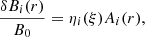
We performed a numerical study of field line transport in the presence of magnetic turbulence. By definition, a magnetic field line at each point in space is tangent to the magnetic field, and this implies that the elementary displacement dr along the field line is parallel to B(r). This can be expressed by writing dr = Bdλ, where dλ is a scalar quantity. Choosing dλ as ds/|B|, we obtain the field line equations as dr/ds = B/|B|, where ds is the arc length element along B. On the other hand, considering dλ as dξB0, with B0 a constant, this yields
 (1)
(1)
where the magnetic field B(r) is given by the average field B0 = B0z(r) plus the fluctuation magnetic field δB(r). We traced the magnetic field lines in the heliosphere, using as average field the Parker spiral field, and integrating the above equation in a local Cartesian frame with the two-axis along B0, where a three-dimensional model of magnetic turbulence allows us to evaluate a nonquasilinear magnetic field line diffusion coefficient even in the case of anisotropic turbulence, as observed in the solar wind. By means of a Monte Carlo (MC) simulation, where a random force term proportional to the diffusion coefficient is added to the magnetic field line equations, we evaluated how the magnetic field lines diffuse with respect to the average field.
2.1. Monte Carlo simulation
The Monte Carlo code gives a random displacement of the simulated field line at each step of the integration along the Parker magnetic field model. The fluctuating field component is modeled as a random process,
 (2)
(2)
where i = x, y; ηx(ξ) and ηy(ξ) are two uncorrelated random functions, and 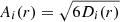 represents the random force amplitudes (Veltri et al. 1998; Ippolito et al. 2005). For each position on the magnetic field line, this random displacement is proportional to a local diffusion coefficient that quantifies the local transport of magnetic field lines and takes the fluctuation level and the main features of the anisotropy of the solar wind turbulence into account (Pommois et al. 2001). The local frame in the solar wind is defined as follows: the z direction is along the local average interplanetary magnetic field B0, the x direction is normal to the plane formed by the radial direction (solar wind speed direction) and B0, and the y direction completes the right-handed system. Because the scale of variation of the average spiral field is much larger than the correlation length of the magnetic turbulence, we can evaluate the diffusion coefficients of magnetic field lines in a local frame in Cartesian geometry as follows:
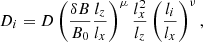 (3)
(3)
where i = x, y and D, μ and ν are dimensionless parameters. A best fit of the computed diffusion coefficient yields D = 0.028, μ = 1.51, and ν = 0.67 (Veltri et al. 1998; Zimbardo et al. 2000; Pommois et al. 2001). The values of lx, ly, and lz represent the turbulence correlation lengths the in the x, y, and z directions and quantify the anisotropy of turbulence in the solar wind. The typical fluctuation levels relevant to the solar wind are δB/B0 ≃ 0.5 ÷ 1 (Zank et al. 1998); the corresponding degrees of anisotropy are lx/ly = 1 ÷ 10, lz/ly = 1 ÷ 10. Our simulation is tailored to each specific event by using the observed values of solar wind velocity and of the level of magnetic fluctuation at Mercury. The model computes the magnetic connection to the solar corona (four solar radii) starting from Mercury’s magnetosphere (≃0.38 AU).
2.2. Evaluation of the magnetic fluctuations
Interplanetary magnetic field data were obtained from MAG-MESSENGER through the database server AMDA1. To evaluate the level of fluctuations within the inertial range, which gives the main contribution to the field line random walk on the relevant time scales, we used the EMD. Given a time series x(t), the EMD allows us to write it as
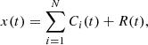 (4)
(4)
where Ci(t) is an oscillating component modulated both in amplitude and in phase, and R(t) is a monotonic function of time, representing the residue of the decomposition (Huang et al. 1998). Each empirical mode or intrinsic mode function Ci(t) is derived via an iterative process called sifting process, which directly acts in the time domain rather than working in a conjugate one (as for Fourier or wavelet analysis). This gives the EMD an adaptive character that is particularly suitable to preserve the nonlinearity and nonstationarity properties of the original time series x(t). The sifting process acts on time series by exploiting its local properties as summarized below:
-
the first step is to subtract the average from x(t) to derive a zero-mean signal;
-
the local maxima and minima are identified and separately interpolated using a cubic spline defining the so-called upper and lower envelope;
-
the average envelope is then evaluated and subtracted from the zero-mean signal;
-
if the obtained signal has the same (or differing at most by one) number of extrema and zero crossings and a zero-average mean envelope, then it is identified as an intrinsic mode function, otherwise, the previous steps are iterated until these two properties are met.
The procedure stops when no more oscillating components can be extracted, thus obtaining the residue R(t) of the decomposition. For more details, we refer to Huang et al. (1998). The derived empirical modes can be now written as modulated in amplitude and phase by means of the Hilbert transform (HT) such that
![Mathematical equation: $$ \begin{aligned} C_{i}(t)=A_{i}(t)\cos [\Phi _{i}(t)], \end{aligned} $$](/articles/aa/full_html/2022/04/aa42328-21/aa42328-21-eq6.gif) (5)
(5)
where Ai(t) and Φi(t) are the so-called instantaneous amplitude and phase of the ith empirical mode. This is the main difference between the EMD and fixed-basis decomposition (such as wavelets): we can derive amplitudes and phases that are time dependent and thus are particularly suitable for nonstationary signals (such as the magnetic field measurements by MESSENGER). Furthermore, the definition of instantaneous frequency immediately follows from the instantaneous phase,
 (6)
(6)
from which a mean timescale of the oscillation for each empirical mode can be derived as
 (7)
(7)
Finally, when the procedure is complete, we can use partial sums of Eq. (4) to reconstruct the dynamics in a specific range of timescales (or frequencies) by summing all empirical modes with τi ∈ [τl, τu]. As shown in Alberti et al. (2021), the inertial range in the vicinity of Mercury is confined between timescales of about 1 s up to 5 × 10² s. We therefore evaluate the level of fluctuations within the inertial range by summing empirical modes whose mean timescales are within this range. The term δB/B0, which constitutes one of the input parameters of our MC simulation, corresponds then to the average of the single values of magnetic fluctuations over the mean field B0 measured by MAG-MESSENGER.
3. Data selection
For the solar wind velocity, data taken by Advanced Composition Explorer (ACE) satellite and provided by the Omniweb at the National Space Science Data Center were used2. At any given time, the planet Mercury is immersed in a plasma stream with variable speed. Clearly, we do not know the solar wind speed along the field lines that are magnetically connected to the planet. Thus, we do not know a priori which solar wind speed Vsw to use to determine the Parker spiral. For each case study, we computed the average solar wind speed Vsw for the 6 days before the occurrence of the considered event and for the 4 days after. When the average solar wind speed is within the limit of the slow wind, and never above 550 km s−1, the uncertainty on the large-scale magnetic structure of the solar wind can be neglected. We selected seven case studies for which a strong enhancement in the solar proton fluxes in the Hermean environment was detected by MESSENGER. For these events, an increase is observed in the solar protons in the energy channel between 12.9 keV and 14.1 keV measured by FIPS-MESSENGER of at least two orders of magnitude from the average value recorded in the previous 27 days, which most probably is induced by the occurrence of a CME cataloged by Winslow et al. (2015). For all the considered events, we additionally analyzed proton fluxes in the energy channel between 0.8 MeV and 2 MeV measured by EPS/MESSENGER. For each of the selected cases, observed on 4 March 2012, 5 June 2011, 12 July 2012, 20 September 2012, 26 May 2012, 27 January 2012, and 21 June 2013, we reconstructed the magnetic connection from Mercury to the solar corona, identifying the contour levels of the distribution of interplanetary magnetic field line footpoint at the solar corona source surface (here assumed to be at 4 solar radii). All the studied events were observed in a quite low solar activity period, at the beginning of solar cycle 24. A further point to study is where Mercury’s orbit intersects the current sheet because this determines whether the planet is located within a positive or negative magnetic sector, that is, a magnetic field outward or inward from the Sun (Russell 2001). For this purpose, the Source Surface Synoptic Charts3 produced by the Wilcox Solar Observatory (WSO) were considered. To produce these magnetic maps of the Sun, the coronal magnetic field, computed using photospheric field observations with a potential field model, is forced to be radial at the source surface to approximate the effect of the accelerating solar wind on the field configuration. The WSO provides magnetic maps that are recorded for each Carrington cycle, so that we have a ϕ coordinate that extends from 0 to 360°. These magnetic maps are computed on the base of the portion of the solar disk that is visible from the Earth. When the relative orbital positions of planets Mercury and the Earth are considered at the time when the solar proton fluxes enhancement is observed at Mercury, the angular distance between the two planets can be computed. By considering 27 days as the mean rotation period of the Sun as seen from the Earth, we can assume that on each day, a specific point on the solar surface covers an angular distance of about 13°. As an example, when the angular distance between Mercury and the Earth is about Δα = 65°, it means that each point on the solar surface covers this distance in about Δα/13 = 5 days. In addition, considering that sunspots typically last for more than one Carrington rotation, it can be assumed that the whole solar disk seen by Mercury at the time when the studied event is observed by MESSENGER is approximately the same as seen from the Earth about 5 days later. This assumption allowed us to project the magnetic footpoint computed for the planet Mercury on the magnetic maps measured from the Earth and provided by the WSO. For all the analyzed cases, the contour levels representing a magnetic footpoint of Mercury, as obtained from the MC simulation, were plotted in heliographic latitude and longitude on the background of the magnetic field map (magnetogram) at the source surface of the solar wind (r = 2.5 R⊙) for the period relevant to the considered event. We computed the footpoint of the Parker spiral passing Mercury, considering the fluctuation levels of the IMF in the two days preceding the analyzed event, in order to study the background conditions of the solar wind magnetic field before the occurrence of the CME. We then compared it with the magnetic footpoint of the planet computed taking the perturbation of the interplanetary medium induced by the CME shock into account, considering the fluctuation level of the IMF on the day of the observed increase in the proton fluxes. This comparison gives us information about the entity of the perturbation of the IMF field lines caused by the passage of the CME shock. Furthermore, the time profile of the protons in the range between 12.9 keV and 14.1 keV is presented together with the spectrogram of the considered SEP event, as retrieved from FIPS-MESSENGER data through the database server AMDA4. The 0.8−2 MeV proton time profiles are also reported, as obtained from EPS/MESSENGER data provided by the Planetary Plasma Interactions (PPI) Node of the Planetary Data System (PDS)5.
4. Results and discussion
We analyzed data acquired by FIPS/MESSENGER during 2011, 2012, and 2013 and studied the time profiles of the proton fluxes with energy within the range 12.9 keV−14.1 keV. We selected seven cases for which an increase in the proton fluxes of at least two orders of magnitude with respect to the background level is observed. Furthermore, proton fluxes in the energy range between 0.8 MeV and 2 MeV measured by EPS/MESSENGER were taken into account for the selected cases. For all the studied events, an enhancement of at least one order of magnitude from the average value recorded in the previous 27 days was also observed in the solar protons detected by EPS/MESSENGER. Using the procedure described above, we considered the magnetic fluctuations in the solar wind in the two days previous to the event as well as the fluctuations on the day when the CME cataloged by Winslow et al. (2015) was observed. This procedure allowed us to retrieve the magnetic footpoint of the planet just before the passage of the CME, as well as the magnetic footpoint after the disturbances induced by the passage of the CME shock wave. The MC simulation gives us a set of contour lines projected on the solar disk as output that represent the probability density distribution of the magnetic field lines connecting Mercury to the solar corona. Blue contour lines in the following plots represent the computed magnetic footpoint of the planet, taking into account the turbulence level observed in the solar wind in the two days before the considered event, while the green contour lines describe the magnetic footpoint of Mercury after the passage of the interplanetary shock due the CME. From the relative position of Mercury and the Earth on the day on which the CME was observed by Winslow et al. (2015), we computed the angular distance between the two planets, and, as discussed above, we were able to project the computed footpoints on the magnetic map provided by WSO. The projection on the magnetogram of the footpoint, the active region coordinates, and the planet position allowed us to evaluate whether Mercury’s magnetic footpoint area and the flare lie on opposite sides of the magnetic equator. This would imply that a sector boundary is found between the flare and the planet, and it is well known that sector boundaries are an obstacle to particle propagation (Kallenrode 1993). At a sector boundary, the average magnetic field direction changes from sunward to antisunward, or vice versa, causing a strong deflection in particle propagation. When the angular distance between the two planets is smaller than ±90°, we considered that measures taken from the Earth at the time when the enhancements in the proton fluxes is observed can also be used.
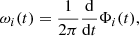
For three out of the seven selected cases (4 March 2012, 12 July 2012, and 21 June 2013) we were able to enrich our analysis by using data taken from satellites at L1 and from ground-based instruments. In two of these events, the very close angular distance between Mercury and the Earth, 31° and 12° for 12 July 2012 and 21 June 2013, respectively, allowed us to conduct a more detailed study. We also computed the magnetic footpoint of the Earth and compared it with the footpoint reconstructed for Mercury. For the enhancements in the proton fluxes recorded by MESSENGER on 5 June 2011, 20 September 2012, 27 January 2012, and 26 May 2012, the angular distance between Earth and Mercuy was quite large, as shown in the left panels of Fig. 1. This makes solar observations taken by spacecraft at L1 inaccurate, if not unusable. In the first two cases, 5 June 2011 and 20 September 2012, a strong increase in the proton fluxes between 12.9 keV and 14.1 keV measured by FIPS/MESSENGER is observed, as shown in the first two right panels from the top of Fig. 1. The two lower panels on the right side of the same figure show a clear enhancement in the same energy channel fluxes recorded on 27 January 2012 and 26 May 2012, although it is not as pronounced as for the 5 June 2011 and 20 September 2012 events. The vertical red lines in the FIPS proton flux time-profile plots represent the arrival time at MESSENGER of the CME observed by Winslow et al. (2015). On 20 September 2012, two CMEs have been observed by the authors, as described by the two vertical red lines in the plot. This is also reflected in the two marked peaks. Although not as pronounced as in the keV channel energy, a clear enhancement is also observed in the same periods for the proton fluxes in the range between 0.8 and 2 MeV measured by EPS/MESSENGER, as shown in Fig. 2. Figures 1 and 2 show strong variability in the peak intensity of energetic particles and in the timing between the CME passage and the energetic particle peak. This variability is also found in observations of energetic particles in the vicinity of Earth (see, e.g., Lee et al. 2012). This can depend on several factors, such as the instrinc variability of the SEP source, the geometry of the magnetic connection between the SEP source and the spacecraft, the fact that energetic particles can be accelerated by both the flare in the corona and the interplanetary CME-driven shock wave, and the fact that propagation regimes different from scatter free or diffusive also exist (see, e.g., Trotta et al. 2020; Prete et al. 2021).
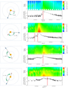 |
Fig. 1. Relative position of planet Mercury (red circle) and the Earth (blue circle), left panels, from top to bottom, for the events on 5 June 2011, 20 September 2012, 27 January 2012, and 26 May 2012. Right panels: enhancements in the particle fluxes observed on the same days that were described by the spectrogram and the proton flux measured by FIPS-MESSENGER in the energy channel between 12.9 and 14.1 KeV. The vertical red line in the proton time profiles represents the CME arrival at MESSENGER (Winslow et al. 2015). The spikes in the time profiles preceding and following the considered events are due to the periodic passage of MESSENGER through Mercury’s magnetosphere. |
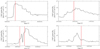 |
Fig. 2. Proton fluxes measured by EPS/MESSENGER in the energy range between 0.8 and 2 MeV on 5 June 2011 and 20 September 2012 are shown in the left panels from top to bottom. Right panels: same particle fluxes observed by EPS/MESSENGER on 27 January 2012 and 26 May 2012 from top to bottom. The vertical red line in the proton time profiles represents the CME arrival at MESSENGER (Winslow et al. 2015). |
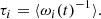
Considering that sunspots typically last for more than one Carrington rotation, and assuming that any point on the Sun surface covers an angular distance of about 13° per day, starting from active region observations taken at L1, we reconstructed the solar disk as seen from Mercury together with the magnetogram based on the Source Surface Synoptic Charts produced by the WSO. Although the great angular distance between the two planets on the days on which the events presented above occurred makes this procedure less accurate, the computing of the magnetic footpoint of the Parker spiral still represents important information for studying the increase in the proton fluxes measured at Mercury. In the panels of Fig. 3, the contour lines representing the area on the solar surface that is magnetically connected to the planet Mercury are plotted, projected on the related magnetogram. From top to bottom, we report the Parker spiral footpoints for the events observed on 5 June 2011, 20 September 2012, 27 January 2012, and 26 May 2012. Computing the magnetic footpoint of Mercury before the occurrence of the CME (blue contour lines in the panel of Fig. 3) and after the passage of the CME shock wave (green contour lines in the panel of Fig. 3) for three over the four cases presented in Fig. 3, we observe, as expected, that a wider region on the solar disk is magnetically connected with the planet. This diffusion of the magnetic field lines connecting Mercury to the solar corona is due to the strong levels of turbulence found in the solar wind, which are amplified by the passage of the CME. For the event on 5 June 2011 (see the top panel of Fig. 3), no particular difference can be noticed between the two footpoints. This can suggest that the CME shock does not immediately reach the field lines connected with the planet, causing only weak disturbances in the region of the interplanetary medium where the magnetic field lines connecting Mercury to the solar corona were located. For the remaining three cases, characterized by an enhancement in the proton flux time profiles observed on 4 March 2012, 12 July 2012, and 21 June 2013 (see right panels of Figs. 4 and 5), the angular distance between the Earth and Mercury were within the interval of ±90°, as shown in the left panels of Fig. 4. This made the reconstruction of the solar disk and the magnetograms centered on Mercury on the days of the events more accurate, which were based on data taken at L1 and from ground-based instruments.
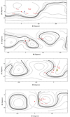 |
Fig. 3. Magnetic footpoints of Mercury plotted on the solar surface (4 solar radii) with contour lines. The footpoints were computed, from top to bottom, for 5 June 2011, 20 September 2012, 27 January 2012, and 26 May 2012. Each panel also reports the relative position of Mercury (red spot) and of the solar active regions (red asterisks), all projected on the solar magnetic configuration at the source surface (r = 2.5 R⊙) magnetograms as seen by the planet, and retrieved from the Wilcox Solar Observatory data. Blue contour lines represent the magnetic footpoint of Mercury before the occurrence of the CME, computed with the values of the IMF recorded by MAG-MESSENGER on the two days before the event. The φ coordinate represents the heliospheric longitude considering a complete Carrington rotation (360°). The zero is set in correspondence of the planet projection on the solar disk. The ϑ coordinate is the heliospheric latitude. Solid green contour lines represent the magnetic footpoint of the planet after the occurrence of the CME, computed with the values of the IMF recorded by MAG-MESSENGER on the day when the event was observed. The thick solid line represents the magnetic equator of the Sun. |
As for the previous events, in Fig. 6 we report from top to bottom the contour lines representing Mercury’s magnetic footpoints computed for the events of 4 March 2012, 12 July 2012, and 21 June 2013. Because the two planets were relatively close to each other, we were able to retrieve the magnetic configuration of the Sun more accurately, together with the position of the active regions seen by the planet Mercury at the time when the events were observed. Figure 6 shows that for all the reported cases, the width of the footpoint area grows with the magnetic fluctuation level. The area described by the green contour lines, representing the magnetic footpoint of Mercury after the occurrence of the CME, computed with the values of IMF recorded by MAG-MESSENGER on the day on which the event was observed, is much wider than the area occupied by the blue contour lines, which constitute the magnetic footpoint of the planet before the occurrence of the CME. For the event on 12 July 2012, this is much more evident, reflecting a very strong perturbation in the solar wind induced by the passage of the CME shock wave. The enhancements in the proton fluxes measured by FIPS/MESSENGER on 12 July 2012 and in the protons at higher energy observed by EPS/MESSENGER on the same day are most probably related to a CME associated with an M-class flare, as cataloged by NOAA, observed on 4 March 2012 on the eastern limb of the solar disk (N19E61) seen by the Earth. The active region site of the flare was AR 11429. The top panel of Fig. 6 shows that AR 11429 is the nearest active area to the regions of the solar surface that are magnetically connected to planet Mercury, and it lies less than 20° in latitude from the magnetic footpoint we computed. This difference in angle is most probably due to diffusion in the solar corona of the particles accelerated on the flare site.
For the 12 July 2012 event, we were also able to identify the active region in which the flare associated with the CME occurred that probably caused the increase in the solar proton fluxes. The NOAA flare catalog data show that an X Class flare, related to a CME, was observed, coming from active region 11520. The middle panel of Fig. 6 clearly shows that the projection of active region 11520 is less than 10° away from Mercury’s magnetic footpoint of the Parker spiral at 4 solar radii.
In the 21 June 2013 event, an M-class flare, most probably related to the occurrence of the CME cataloged by Winslow et al. (2015), which caused the enhancements in the solar protons fluxes, has been observed coming from active region 11777. Despite the great distance of the flare site from the planet’s footpoint, as shown in the lower panel of Fig. 6, intense proton fluxes have been observed at Mercury. The proton time profiles as well as the spectrogram show a narrow peak on 21 June 2013 (see Figs. 4 and 5). These considerations suggest that these particles were probably accelerated by the CME shock propagating through the interplanetary medium, and not at the flare site. In addition, the observed CME was characterize by a shock transit speed of 1290 km s−1, as reported by Winslow et al. (2015). The shock could have reached the magnetic field lines connected to Mercury in a very short time, allowing the particles accelerated in this portion of the interplanetary medium to arrive at the spacecraft quite soon. This is also reflected in the time delay observed by Winslow et al. (2015) between the time at which the CME was observed at the Sun (02:54 UT) and the time at which the CME hit the planet (17:37 UT). Furthermore, the proximity of Mercury to the Sun may introduce a further instrumental problem in distinguishing particles accelerated by flares from those accelerated by CME shocks.
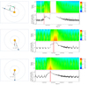 |
Fig. 4. As Fig. 1 but for the events (from top to bottom) observed on 4 March 2012, 12 July 2012 and 21 June 2013. |
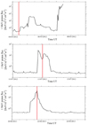 |
Fig. 5. As Fig. 2 but for the events (from top to bottom) observed on 4 March 2012, 12 July 2012 and 21 June 2013. |
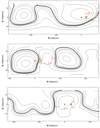 |
Fig. 6. As Fig. 3, but for the events (from top to bottom) observed on 4 March 2012, 12 July 2012, and 21 June 2013. |
For the last two cases presented, which occurred on 12 July 2012 and 21 June 2013, the very close angular distance between the Earth and Mercury (see the middle and lower panels on the left side of Fig. 4) allowed us to conduct a more detailed analysis of the events. We also reconstructed for the same days the magnetic footpoint of the Earth. The magnetic connection from the Earth to the solar corona (4 solar radii) was computed with the same technique as discussed above. The comparison of the footpoint of the Parker spiral of the two planets is reported in Fig. 7. The two panels of Fig. 7 show a much larger spread of the magnetic field lines that connect the Earth to the solar corona than those that connect to the magnetic footpoint of Mercury. This effect is mainly due to the combination of a quite slow solar wind (447 km s−1 and 344 km s−1 on average, respectively) measured in the four days before the analyzed events, together with the levels of turbulence measured at 1 AU and the greater radial distance from the Sun. In the case study of 12 July 2012, active region 11520, in which the X-class flare probably related to the CME cataloged by Winslow et al. (2015) has been observed, is quite far from the area on the solar corona that is magnetically well connected to the Earth (see top panel of Fig. 7). This might explain why no particularly strong enhancements in the proton fluxes with energy E >10 MeV and E >30 MeV are observed at L1, as reported in the lower panel on the right side of Fig. 8. In addition, the increases in these fluxes are observed several hours after the peak in the proton fluxes observed at Mercury, as shown in the plots of the top panels on the right side of the same figure. The reason most likely is that in its expansion in the interplanetary medium, it took several hours for the CME shock to reach the magnetic field lines connected with the Earth. Furthermore, the projection of the Earth’s magnetic footpoint on the magnetogram shows that it lies in two magnetic sectors of opposite polarity, and this could inhibit the propagation of the particles in the interplanetary medium. For the event of 21 June 2013, the lower panel of Fig. 7 shows that active region 11777, the site at which the M-class flare probably related to the CME was observed, is even farther from the magnetic footpoint of the Earth than that of Mercury. When we also consider the greater distance of the Earth from the Sun, no particularly intense fluxes of solar protons have been recorded at L1, as demonstrated by the small enhancement in the proton fluxes with energy E >10 MeV and E >30 MeV reported in the bottom panel on the right side of Fig. 8.
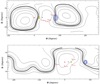 |
Fig. 7. Magnetic footpoints of the Earth (blue contour lines) and Mercury (green contour lines) from top to bottom, computed for 12 July 2012 and 21 June 2013. We also report the relative position of Mercury (red circle) and of the Earth (blue square) projected on the solar magnetic configuration at the source surface (r = 2.5 R⊙) magnetograms as seen by Mercury, and retrieved from WSO data. |
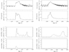 |
Fig. 8. Proton flux in the range between 12.9 and 14.1 keV observed on 12 July 2012 by FIPS-MESSENGER, proton flux in the range between 0.8 and 2 MeV retrieved from EPS/MESSENEGER data on 12 July 2012, and the proton fluxes >10 MeV and 30 MeV, measured at L1 for the same day as obtained from the OMNIWEB data explorer website (left panels, top to bottom). Same quantities in the same order, but for the 21 June 2013 event (right panels). |
5. Conclusions
A numerical simulation based on a Monte Carlo code was carried out in order to reconstruct the magnetic connection from planet Mercury to the solar corona in correspondence to specific SEP events. The random walk of the interplanetary magnetic field lines, due to the low-frequency turbulence in the solar wind, was modeled through local diffusion coefficients, which are functions of the measured magnetic fluctuation in the solar wind, and which are also related to the correlation length of the magnetic turbulence (Veltri et al. 1998; Zimbardo et al. 2000). The fluctuation levels of the interplanetary magnetic field were retrieved from MAG-MESSENGER data and computed applying the EMD method by summing empirical modes whose mean timescales are within 1 s up to 5 × 10² s. This allowed us to distinguish the magnetic field fluctuations inside Mercury’s environment from those in the solar wind. We studied the proton fluxes measured by FIPS-MESSENGER during 2011, 2012, and 2013 and selected seven cases in which an increase of at least two orders of magnitude from the typical values recorded in the previous 27 days were observed. Data related to proton fluxes in the energy channel between 0.8 and 2 MeV acquired by EPS/MESSENGER were also studied for each of the selected cases. The footpoint of the Parker spiral passing Mercury was reconstructed for all of the selected events. For each of them, we computed the contour levels of the distribution of interplanetary magnetic field lines at the solar wind source surface, which represent the magnetic footpoint of the planet. By considering the values of fluctuation levels of the IMF recorded by MAG-MESSENGER two days before the event and the values of fluctuation levels of the IMF on the day on which the event was observed, we were also able to appreciate the effects on the solar wind magnetic field perturbations induced by the CME shock. For each of the seven case studies, the relative position of Mercury, the planet’s magnetic footpont area computed by the simulation, together with the active regions sites, were projected on the solar magnetic configuration at the source surface (r = 2.5 R⊙) WSO magnetograms.
In the relation between the magnetic connection from Mercury to the solar corona and the solar active regions related to the proton acceleration for the events observed on 5 June 2011, 20 September 2012, 27 January 2012, and 26 May 2012, no direct comparison with the Earth can be made. Because of the high relative angular distance between Mercury and the Earth, observations of the solar corona taken from the Earth cannot be used reliably. However, the reconstruction of the magnetic footpoint of Mercury after the passage of the CME shows a wider spread in space of the field lines connecting the planet to solar corona because the fluctuation levels in the IMF introduced by the passage of the shock wave are higher.
For three events observed on 4 March 2012, 12 July 2012, and 21 June 2013, the relatively low angular distance between Mercury and the Earth allowed us to conduct an accurate analysis of the solar data coming from Earth-based instruments, together with data obtained by different spacecraft at L1. For the increase in the proton fluxes measured on 4 March 2012, the CME that probably caused the event was associated to an M-class flare that was observed on the eastern limb of the solar disk seen by the Earth, coming from the active region that was nearest to the area of the solar surface that was magnetically connected to the planet.
For the 12 July 2012 event, an angular difference of about 10° is observed between the reconstructed Mercury nominal magnetic footpoint and the active region in which the flare occurred that was related to the CME that probably caused the increase in the solar proton fluxes. In the case study of 21 June 2013, an M-class flare, most probably related to the occurrence of the CME cataloged by Winslow et al. (2015) that was responsible for the enhancements in the solar protons fluxes, was recorded. This solar flare has been observed to come from an active region on the east side of the solar disk seen by Mercury, and far from the area on the solar surface magnetically connected to the planet that we computed. In addition, the enhancement in the proton fluxes described by the spectrogram and the proton time profiles measured by MESSENGER show a narrow peak, likely because the particles were accelerated by the CME shock propagating through the interplanetary medium (compare the intensity profile with the profiles obtained by Prete et al. 2019), and not at the flare site. Furthermore, the high transit speed of the shock (1290 km s−1 as reported by Winslow et al. 2015) allowed the shock wave to reach the magnetic field lines connected to Mercury in a short time, causing the intense proton fluxes measured by the spacecraft.
For the case studies of 12 July 2012 and 21 June 2013, due to a very small angular distance between Mercury and the Earth (31° and 12° respectively) we were able to perform a more detailed analysis. For the same day, we compared the magnetic footpoint of Mercury and the magnetic footpoint of the Earth. For both events, the greater angular distance of the Earth’s magnetic footpoint from the site of the flare probably associated with the observed CME, explains the low proton fluxes observed at L1 compared to the strong enhancement in the suprathermal protons observed at Mercury.
This study shows that the simulation described by Ippolito et al. (2005) is also valid when the solar wind magnetic fluctuation level is estimated indirectly by MESSENGER, using the EMD technique. It also shows that a high-quality CME catalog such as that of Winslow et al. (2015) can be used to study the propagation of SEPs and to envision the likely acceleration source. This method of analysis complements methods based on global MHD simulations such as ENLIL, and it could be applied to the BepiColombo measurements during the next Mercury flybys (Mangano et al. 2021), as well as during the nominal mission phase. Further information about the active regions could be obtained not only from the ground, but also from the diverse spacecraft operating in the inner Solar System, such as Solar Orbiter (Müller et al. 2013), the Parker Solar Probe (Fox et al. 2016), and Stereo A (Wuelser et al. 2004). Therefore, we will have many chances to observe SEP events at Mercury and to study them in detail in the next years.
Acknowledgments
The authors acknowledge the AMDA database (http://amda.cdpp.eu); the Planetary Data System (PDS) (https://pds.nasa.gov); the SPDF OMNIWeb database (https://omniweb.gsfc.nasa.gov); the Wilcox Solar Observatory database (http://wso.stanford.edu); the Planetary Plasma Interactions (PPI) Node of the Planetary Data System (PDS) (https://pds-ppi.igpp.ucla.edu/search/view/?id=pds://PPI/mess-epps-eps-calibrated).
References
- Alberti, T., Milillo, A., Laurenza, M., et al. 2021, Front. Phys., 9, 668098 [CrossRef] [Google Scholar]
- Arge, C. N., & Pizzo, V. J. 2000, J. Geophys. Res.: Space Phys., 105, 10465 [NASA ADS] [CrossRef] [Google Scholar]
- Arge, C. N., Luhmann, J. G., Odstrcil, D., et al. 2004, J. Atmos. Solar-Terr. Phys., 66, 1295 [NASA ADS] [CrossRef] [Google Scholar]
- Bavassano, B., Dobrowolny, M., Mariani, F., & Ness, N. F. 1982, J. Geophys. Res.: Space Phys., 87, 3617 [NASA ADS] [CrossRef] [Google Scholar]
- Belcher, J. W., & Davis, L., Jr. 1971, J. Geophys. Res.: Space Phys., 76, 3534 [NASA ADS] [CrossRef] [Google Scholar]
- Dewey, R. M., Baker, D. N., Anderson, B. J., et al. 2015, J. Geophys. Res.: Space Phys., 120, 5667 [NASA ADS] [CrossRef] [Google Scholar]
- Fox, N. J., Velli, M. C., Bale, S. D., et al. 2016, Space Sci. Rev., 204, 7 [Google Scholar]
- Gershman, D. J., Slavin, J. A., Raines, J. M., et al. 2015, J. Geophys. Res.: Space Phys., 120, 4354 [NASA ADS] [CrossRef] [Google Scholar]
- Huang, N. E., Shen, Z., Long, S. R., et al. 1998, Proc. R. Soc. London Ser. A, 454, 903 [NASA ADS] [CrossRef] [Google Scholar]
- Ippolito, A., Pommois, P., Zimbardo, G., & Veltri, P. 2005, A&A, 438, 705 [NASA ADS] [CrossRef] [EDP Sciences] [Google Scholar]
- Jackson, B. V., & Hick, P. P. 2004, Solar and Space Weather Radiophysics (Dordrecht: Springer), 314 [Google Scholar]
- Jokipii, J. R., & Parker, E. N. 1968, Phys. Rev. Lett., 21, 44 [NASA ADS] [CrossRef] [Google Scholar]
- Kallenrode, M. B. 1993, JGR Space Phys., 98, 19037 [NASA ADS] [Google Scholar]
- Leblanc, F., Luhmann, J. G., Johnson, R. E., & Liu, M. 2003, Planet. Space Sci., 51, 339 [NASA ADS] [CrossRef] [Google Scholar]
- Lee, M. A., Mewaldt, R. A., & Giacalone, J. 2012, Space Sci. Rev., 173, 247 [CrossRef] [Google Scholar]
- Mangano, V., Dósa, M., Fränz, M., et al. 2021, Space Sci. Rev., 217, 23 [NASA ADS] [CrossRef] [Google Scholar]
- Milillo, A., Mangano, V., Massetti, S., et al. 2021, Icarus, 355, 0019 [Google Scholar]
- Müller, D., Marsden, R. G., St. Cyr, O. C., et al. 2013, Sol. Phys., 285, 25 [Google Scholar]
- Odstricil, D. 2003, Adv. Space Res., 32, 497 [CrossRef] [Google Scholar]
- Plainaki, C., Lilensten, J., Radioti, A., et al. 2016, J. Space Weather Space Clim., 6, A31 [NASA ADS] [CrossRef] [EDP Sciences] [Google Scholar]
- Pommois, P., Veltri, P., & Zimbardo, G. 2001, J. Geophys. Res.: Space Phys., 106, 24965 [NASA ADS] [CrossRef] [Google Scholar]
- Prete, G., Perri, S., & Zimbardo, G. 2019, Adv. Space Res., 63, 2659 [NASA ADS] [CrossRef] [Google Scholar]
- Prete, G., Perri, S., & Zimbardo, G. 2021, New Astron., 87, 101605 [NASA ADS] [CrossRef] [Google Scholar]
- Pucci, F., Malara, F., Perri, S., et al. 2016, MNRAS, 459, 3395 [NASA ADS] [CrossRef] [Google Scholar]
- Reames, D. V. 2013, Space Sci. Rev., 175, 53 [CrossRef] [Google Scholar]
- Russell, C. T. 2001, Geophys. Monogr. Ser., 125, 73 [NASA ADS] [Google Scholar]
- Trotta, D., Burgess, D., Prete, G., Perri, S., & Zimbardo, G. 2020, MNRAS, 491, 580 [NASA ADS] [CrossRef] [Google Scholar]
- Veltri, P., Zimbardo, G., & Pommois, P. 1998, Adv. Space Res., 22, 55 [NASA ADS] [CrossRef] [Google Scholar]
- Winslow, R. M., Lugaz, N., Philpott, L. C., et al. 2015, J. Geophys. Res.: Space Phys., 120, 6101 [Google Scholar]
- Wuelser, J.-P., Lemen, J. R., Tarbell, T. D., et al. 2004, Telesc. Instrum. Sol. Astrophys., 5171, 111 [NASA ADS] [CrossRef] [Google Scholar]
- Zank, G. P., Matthaeus, W. H., Bieber, J. W., & Moraal, H. 1998, J. Geophys. Res.: Space Phys., 103, 2085 [NASA ADS] [CrossRef] [Google Scholar]
- Zimbardo, G., Veltri, P., & Pommois, P. 2000, Phys. Rev. E, 61, 1940 [NASA ADS] [CrossRef] [Google Scholar]
All Figures
|
Fig. 1. Relative position of planet Mercury (red circle) and the Earth (blue circle), left panels, from top to bottom, for the events on 5 June 2011, 20 September 2012, 27 January 2012, and 26 May 2012. Right panels: enhancements in the particle fluxes observed on the same days that were described by the spectrogram and the proton flux measured by FIPS-MESSENGER in the energy channel between 12.9 and 14.1 KeV. The vertical red line in the proton time profiles represents the CME arrival at MESSENGER (Winslow et al. 2015). The spikes in the time profiles preceding and following the considered events are due to the periodic passage of MESSENGER through Mercury’s magnetosphere. |
| In the text | |
|
Fig. 2. Proton fluxes measured by EPS/MESSENGER in the energy range between 0.8 and 2 MeV on 5 June 2011 and 20 September 2012 are shown in the left panels from top to bottom. Right panels: same particle fluxes observed by EPS/MESSENGER on 27 January 2012 and 26 May 2012 from top to bottom. The vertical red line in the proton time profiles represents the CME arrival at MESSENGER (Winslow et al. 2015). |
| In the text | |
|
Fig. 3. Magnetic footpoints of Mercury plotted on the solar surface (4 solar radii) with contour lines. The footpoints were computed, from top to bottom, for 5 June 2011, 20 September 2012, 27 January 2012, and 26 May 2012. Each panel also reports the relative position of Mercury (red spot) and of the solar active regions (red asterisks), all projected on the solar magnetic configuration at the source surface (r = 2.5 R⊙) magnetograms as seen by the planet, and retrieved from the Wilcox Solar Observatory data. Blue contour lines represent the magnetic footpoint of Mercury before the occurrence of the CME, computed with the values of the IMF recorded by MAG-MESSENGER on the two days before the event. The φ coordinate represents the heliospheric longitude considering a complete Carrington rotation (360°). The zero is set in correspondence of the planet projection on the solar disk. The ϑ coordinate is the heliospheric latitude. Solid green contour lines represent the magnetic footpoint of the planet after the occurrence of the CME, computed with the values of the IMF recorded by MAG-MESSENGER on the day when the event was observed. The thick solid line represents the magnetic equator of the Sun. |
| In the text | |
|
Fig. 4. As Fig. 1 but for the events (from top to bottom) observed on 4 March 2012, 12 July 2012 and 21 June 2013. |
| In the text | |
|
Fig. 5. As Fig. 2 but for the events (from top to bottom) observed on 4 March 2012, 12 July 2012 and 21 June 2013. |
| In the text | |
|
Fig. 6. As Fig. 3, but for the events (from top to bottom) observed on 4 March 2012, 12 July 2012, and 21 June 2013. |
| In the text | |
|
Fig. 7. Magnetic footpoints of the Earth (blue contour lines) and Mercury (green contour lines) from top to bottom, computed for 12 July 2012 and 21 June 2013. We also report the relative position of Mercury (red circle) and of the Earth (blue square) projected on the solar magnetic configuration at the source surface (r = 2.5 R⊙) magnetograms as seen by Mercury, and retrieved from WSO data. |
| In the text | |
|
Fig. 8. Proton flux in the range between 12.9 and 14.1 keV observed on 12 July 2012 by FIPS-MESSENGER, proton flux in the range between 0.8 and 2 MeV retrieved from EPS/MESSENEGER data on 12 July 2012, and the proton fluxes >10 MeV and 30 MeV, measured at L1 for the same day as obtained from the OMNIWEB data explorer website (left panels, top to bottom). Same quantities in the same order, but for the 21 June 2013 event (right panels). |
| In the text | |
Current usage metrics show cumulative count of Article Views (full-text article views including HTML views, PDF and ePub downloads, according to the available data) and Abstracts Views on Vision4Press platform.
Data correspond to usage on the plateform after 2015. The current usage metrics is available 48-96 hours after online publication and is updated daily on week days.
Initial download of the metrics may take a while.