| Issue |
A&A
Volume 660, April 2022
|
|
|---|---|---|
| Article Number | A41 | |
| Number of page(s) | 26 | |
| Section | Stellar structure and evolution | |
| DOI | https://doi.org/10.1051/0004-6361/202142076 | |
| Published online | 07 April 2022 | |
Type II supernovae from the Carnegie Supernova Project-I
II. Physical parameter distributions from hydrodynamical modelling
1
Instituto de Astrofísica de La Plata (IALP), CCT-CONICET-UNLP, Paseo del Bosque s/n, B1900FWA La Plata, Argentina
e-mail: This email address is being protected from spambots. You need JavaScript enabled to view it.
2
Facultad de Ciencias Astronómicas y Geofísicas, Universidad Nacional de La Plata, Paseo del Bosque s/n, B1900FWA La Plata, Argentina
3
Universidad Nacional de Río Negro, Sede Andina, Mitre 630, 8400 Bariloche, Argentina
4
Kavli Institute for the Physics and Mathematics of the Universe (WPI), The University of Tokyo, 5-1-5 Kashiwanoha, Kashiwa, Chiba 277-8583, Japan
5
European Southern Observatory, Alonso de Córdova 3107, Casilla 19, Santiago, Chile
6
Vice President and Head of Mission of AURA-O in Chile, Avda. Presidente Riesco 5335 Suite 507, Santiago, Chile
7
Hagler Institute for Advanced Studies, Texas A&M University, College Station, TX 77843, USA
8
CENTRA-Centro de Astrofísica e Gravitaçäo and Departamento de Física, Instituto Superio Técnico, Universidade de Lisboa, Avenida Rovisco Pais, 1049-001 Lisboa, Portugal
9
Data and Artificial Intelligence Initiative, Faculty of Physical and Mathematical Sciences, University of Chile, Chile
10
Centre for Mathematical Modelling, Faculty of Physical and Mathematical Sciences, University of Chile, Chile
11
Millennium Institute of Astrophysics, Chile
12
Department of Astronomy, Faculty of Physical and Mathematical Sciences, University of Chile, Chile
13
Consejo Nacional de Investigaciones Científicas y Tećnicas (CONICET), Argentina
14
Department of Physics and Astronomy, Aarhus University, Ny Munkegade 120, 8000 Aarhus C, Denmark
15
Carnegie Observatories, Las Campanas Observatory, Casilla 601, La Serena, Chile
16
Finnish Centre for Astronomy with ESO (FINCA), University of Turku, 20014 Turku, Finland
17
Tuorla Observatory, Department of Physics and Astronomy, University of Turku, 20014 Turku, Finland
18
Observatories of the Carnegie Institution for Science, 813 Santa Barbara St., Pasadena, CA 91101, USA
19
Institute for Astronomy, University of Hawaii, 2680 Woodlawn Drive, Honolulu, HI 96822, USA
20
Department of Astronomy, University of California, 501 Campbell Hall, Berkeley, CA 94720-3411, USA
21
Institute of Space Sciences (ICE, CSIC), Campus UAB, Carrer de Can Magrans, s/n, 08193 Barcelona, Spain
22
Department of Physics, Florida State University, 77 Chieftan Way, Tallahassee, FL 32306, USA
23
George P. and Cynthia Woods Mitchell Institute for Fundamental Physics and Astronomy, Department of Physics and Astronomy, Texas A&M University, College Station, TX 77843, USA
Received:
23
August
2021
Accepted:
13
December
2021
Abstract
Linking supernovae to their progenitors is a powerful method for furthering our understanding of the physical origin of their observed differences while at the same time testing stellar evolution theory. In this second study of a series of three papers where we characterise type II supernovae (SNe II) to understand their diversity, we derive progenitor properties (initial and ejecta masses and radius), explosion energy, and 56Ni mass and its degree of mixing within the ejecta for a large sample of SNe II. This dataset was obtained by the Carnegie Supernova Project-I and is characterised by a high cadence of SNe II optical and near-infrared light curves and optical spectra that were homogeneously observed and processed. A large grid of hydrodynamical models and a fitting procedure based on Markov chain Monte Carlo methods were used to fit the bolometric light curve and the evolution of the photospheric velocity of 53 SNe II. We infer ejecta masses of between 7.9 and 14.8 M⊙, explosion energies between 0.15 and 1.40 foe, and 56Ni masses between 0.006 and 0.069 M⊙. We define a subset of 24 SNe (the ‘gold sample’) with well-sampled bolometric light curves and expansion velocities for which we consider the results more robust. Most SNe II in the gold sample (∼88%) are found with ejecta masses in the range of ∼8−10 M⊙, coming from low zero-age main-sequence masses (9−12 M⊙). The modelling of the initial-mass distribution of the gold sample gives an upper mass limit of 21.3 M⊙ and a much steeper distribution than that for a Salpeter massive-star initial mass function (IMF). This IMF incompatibility is due to the large number of low-mass progenitors found – when assuming standard stellar evolution. This may imply that high-mass progenitors lose more mass during their lives than predicted. However, a deeper analysis of all stellar evolution assumptions is required to test this hypothesis.
Key words: supernovae: general / stars: evolution / stars: massive
© ESO 2022
1. Introduction
Core-collapse supernovae (CCSNe) are produced by the explosion of massive stars (> 8 − 10 M⊙). The collapse is initiated when the iron core achieves the Chandrasekhar mass (Chandrasekhar 1939). When the collapsing core reaches nuclear densities, the implosion rebounds, generating a shock wave that stalls into accretion due to the flat density profile around the iron core. However, neutrino heating from the proto-neutron star revives the shock and produces the supernova (SN) explosion. This is the so-called delayed neutrino-driven mechanism, and it is the most favoured explosion mechanism for CCSNe (see e.g. Burrows & Vartanyan 2021, for a recent review).
Type II supernovae (SNe II) are the most common type of CCSN in nature (Li et al. 2011; Shivvers et al. 2017). In the context of single stellar evolution, they are believed to arise from the least massive stars among the core-collapse mechanism. Type II SNe are classified by the presence of hydrogen lines in their optical spectra (Minkowski 1941). Previous theoretical studies have shown that an extensive hydrogen-rich envelope, typical of red supergiant (RSG) stars, is required to reproduce SN II light-curve (LC) morphologies (e.g. Grassberg et al. 1971; Chevalier 1976). More recently, this picture was confirmed by the detection of a significant number of RSG stars at the position of SN II explosion sites on archival images prior to explosion, demonstrating that they are the progenitors of most SNe II (e.g. Van Dyk et al. 2003; Smartt 2009). Type II SNe were historically grouped into SNe IIP and SNe IIL categories based on the shape of their LCs (Barbon et al. 1979). However, in this paper we use ‘SNe II’ to refer to both groups together since recent studies indicate that they come from a continuous population (Anderson et al. 2014a; Sanders et al. 2015; Galbany et al. 2016; Valenti et al. 2016; Rubin & Gal-Yam 2016; de Jaeger et al. 2019, although see Davis et al. 2019 for distinct populations in near-infrared spectral features). Other hydrogen-rich SNe (SNe IIb, SNe IIn, and SN 1987A-like events) are not analysed in this study, and they will not be discussed.
During the last few decades, several works have focused on the analysis of large samples of SNe II to examine their photometric and spectroscopic diversity (e.g. Patat et al. 1994; Hamuy 2003; Bersten & Hamuy 2009; Arcavi et al. 2012; Anderson et al. 2014a,b; Faran et al. 2014a,b; Spiro et al. 2014; González-Gaitán et al. 2015; Gutiérrez et al. 2014, 2017a,b; de Jaeger et al. 2018; Davis et al. 2019). The great diversity observed in SNe II is indicative of a large variety of progenitor and explosion properties. A key aim of SN research is to determine the full range of parameters that produce these events and constrain the predominant physical properties that yield the observed diversity. Obtaining such knowledge is critical to furthering our understanding of how massive stars evolve through their lives to produce hydrogen-rich events, along with the properties of the explosion mechanism.
There are different approaches to connecting the characteristics of SNe with their progenitors (e.g. pre-SN imaging, LC modelling, and nebular-phase spectral modelling), but here we concentrate on those methods that use LCs and spectral information to extract the physical properties of SNe II. Since the pioneering works of Litvinova & Nadezhin (1983, 1985), who presented a set of analytical relations connecting SN observables (the absolute V magnitude and photospheric velocity at mid-plateau and the plateau duration) with progenitor and explosion properties (ejecta mass, progenitor radius, and explosion energy), significant efforts have been made to improve the estimation of confident physical parameters. While the concept of using simple relations to derive progenitor properties is in principle powerful, atypical values have sometimes been obtained (see e.g. Hamuy 2003), motivating advances in this methodology. The hydrodynamical models utilised to calibrate these analytical relations were based on simplified physical assumptions (e.g. simple polytropic models as initial configurations, old opacity tables, and the omission of 56Ni heating in the calculations). Similar relations were presented in Popov (1993), although they were built from a two-zone analytical model for hydrogen recombination in SN II ejecta (see also Arnett 1980, for an analytic analysis for SN II LCs). New analytical relations based on modern hydrodynamical models (including the effects of 56Ni heating and contemporary opacity tables) were presented by Kasen & Woosley (2009) and more recently by Goldberg et al. (2019). While these methods enable the user to extract physical parameters of SNe II in a relatively simple manner, it is not clear how accurate such constraints are because they are obtained using only three observables.
An alternative method for deriving the physical parameters of SNe II consists of detailed modelling of the complete LC evolution – sometimes modelled together with spectral information. In such techniques, the explosion is often simulated by artificially adding internal energy near the centre of the star, known as a ‘thermal bomb’. Here, the structure of the progenitor prior to core collapse has to be assumed, together with the explosion energy, 56Ni yields, and 56Ni distribution within the ejecta (e.g. Utrobin 2007; Bersten et al. 2011; Morozova et al. 2015). These parameters are freely chosen to reproduce the observations. Most studies use hydrodynamical codes that solve the radiation transport in the diffusion approximation, thus producing bolometric LCs. More sophisticated codes incorporate radiation-hydrodynamical modelling with LC and spectral information (Pumo & Zampieri 2011) or multi-group radiative transfer that produces multi-band LC simulations (Blinnikov et al. 1998). Additionally, radiative transfer codes have been developed to calculate spectra in rapidly expanding SN atmospheres, assuming homologous expansion (e.g. Dessart & Hillier 2005; Kasen et al. 2006). Further sophistication can be attained by calculating more realistic explosions using CCSN simulations, parameterising the delayed neutrino-driven mechanism, and coupling this to explosive nucleosynthesis calculations. In this context, the explosion energy, 56Ni mass, and distributions are no longer free parameters. These calculations simulate the collapse and explosion, but they need alternative codes to reproduce SN observables. Recent efforts have been made in this direction (Sukhbold et al. 2016; Curtis et al. 2021; Barker et al. 2021), where multi-dimensional explosions are sometimes mimicked in 1D models and mapped to different codes to further obtain SN observables. While this methodology is more consistent (given that it only needs the progenitor structure as input), sometimes it cannot reproduce the observations and is restricted to a limited parameter space.
Progenitor models can also be constructed in different ways, either as an ad hoc configuration or with detailed stellar evolution from main sequence to core collapse. In general, non-rotating single-star models are used, whereas binarity or stellar evolution with enhanced mass loss could have a significant effect on the structure of the progenitor. Stellar evolution produces a final structure for each star, for which the pre-explosion mass and the progenitor size are not independent. To treat the progenitor final mass and radius as independent parameters, non-evolutionary models – polytropic models – are used (e.g. Utrobin 2007; Bersten et al. 2011). These models can also mimic Rayleigh-Taylor (RT) mixing during shock propagation by smoothing the transitions between zones of different chemical abundances (Utrobin & Chugai 2008). It is important to note that different approaches assumed in the construction of pre-SN models and the subsequent explosion and transient modelling may produce different results because of their assumed physics and the assumed free parameters.
Many studies have been published that show hydrodynamical modelling of individual SNe II. Recently, the number of multiple studies of SNe II has increased (e.g. Pumo et al. 2017; Ricks & Dwarkadas 2019; Utrobin & Chugai 2019; Eldridge et al. 2019; Martinez & Bersten 2019; Martinez et al. 2020). However, there are still only a few analyses of statistically significant samples (González-Gaitán et al. 2015; Morozova et al. 2018; Förster et al. 2018). In Martinez et al. (2020, hereafter M20), we analysed a sample of eight SNe II with observed progenitors by fitting their bolometric LC and photospheric velocity evolution. For this purpose, we presented a large grid of explosion models and a fitting procedure based on Markov chain Monte Carlo (MCMC) methods. We found that our results are consistent with those from pre-SN imaging and late-time spectral modelling. The analysis by M20 served as the basis for the present study, where we derive physical parameters for a large sample of SNe II from a homogeneous dataset.
The present work is the second in a series of three papers based on the study of a sample of 74 SNe II observed by the Carnegie Supernova Project-I (CSP-I; Hamuy et al. 2006). CSP-I was a SN follow-up programme based at the Las Campanas Observatory that obtained high-quality optical and near-infrared (NIR) LCs and optical spectra with high observational cadence. In Martinez et al. (2022a, hereafter Paper I), we calculated the bolometric LCs for this sample of SNe II, discussing our methodology in detail and presenting an analysis of the observed bolometric parameters. An additional conclusion of Paper I is the importance of having NIR observations to derive reliable bolometric luminosities. Here, in Paper II, we assess the progenitor and explosion properties for this sample of events and characterise the physical parameter distributions. Finally, in Martinez et al. (2022b, hereafter Paper III), we study correlations between physical parameters and different LC and spectroscopic measurements, and analyse SN II diversity, tying this to the physics of massive star explosions and their progenitors.
The current paper is organised as follows. In the following section we briefly outline the physical processes involved in SN II explosions. Section 3 describes the data sample. In Sect. 4 we present the hydrodynamical simulations and the fitting procedure used to derive the physical parameters of the sample. Section 5 presents the distributions of the physical parameters for our sample of SNe II. In Sect. 6 we compare our findings with those presented in previous works. In Sect. 7 we discuss possible explanations for the initial mass distribution found. We provide our concluding remarks in Sect. 8. Further analysis and figures not included in the main body of the manuscript are presented in the appendices.
2. SN II physics
The observed behaviour of SN II LCs and expansion velocities is related to physical properties of the progenitor star and the explosion; such as the ejecta mass (Mej), the progenitor radius (R), the explosion energy (E), the amount of 56Ni (MNi), and the distribution of 56Ni in the ejecta (56Ni mixing). Below, different phases of SNe II evolution are discussed in the context of their physical processes. Detailed reviews can be found in the literature (e.g. Arnett 1996; Woosley et al. 2002; Zampieri 2017).
During the core collapse, a powerful shock wave is generated near the centre of the star. The shock wave heats and accelerates the progenitor envelope until it arrives at the stellar surface, where photons begin to diffuse outwards (a phase known as the ‘shock breakout’). After the shock breakout, the outermost layers of the ejecta expand at great speed leading to a fast decrease in the temperature and, therefore, causing a rapid decline in the bolometric luminosity. This phase is commonly known as the ‘cooling phase’, and it is directly related to the progenitor size. However, this phase is also closely related to any material near the stellar surface.
Type II SNe enter the recombination phase when the temperature drops to ∼6000 K. This phase is commonly referred to in the literature as the ‘plateau’, although it is not necessarily a phase of constant luminosity. During this phase, hydrogen recombination takes place at different layers of the ejecta as a recombination wave recedes (in mass coordinate) through the expanding ejecta (e.g. Grassberg et al. 1971; Bersten et al. 2011). Therefore, the hydrogen-rich envelope mass of the progenitor star at the time of explosion (MH, env) is related to the duration of the plateau phase, although other physical parameters also play a role (see Paper III). In addition, the explosion energy significantly drives SN II observational properties (Kasen & Woosley 2009; Dessart et al. 2013; Bersten 2013). More energetic explosions produce more luminous SNe II expanding at higher velocities, thus cooling and recombining the ejecta more rapidly, and producing shorter plateau phases. On the other hand, more extended progenitors produce more luminous and longer plateau phases. The additional heating of the SN II ejecta at late times by the 56Ni decay chain extends the duration of the plateau (Kasen & Woosley 2009) and increases the luminosity in the late-plateau phase (Bersten 2013). The mixing of 56Ni determines when energy deposition from radioactive decay starts to influence the LC, affecting the duration of the plateau and its shape (Bersten et al. 2011; Kozyreva et al. 2019). An extensively mixed 56Ni impacts the LC earlier (see Bersten et al. 2011, their Fig. 12), that is, 56Ni powers the LC sooner, producing a slowly declining plateau (typical SN IIP). The cooling and plateau phases together are also known as the optically thick or photospheric phase.
When the hydrogen-rich ejecta is recombined, SNe II enter a transition phase, which is marked by a rapid decline in luminosity. After this, the luminosity is mainly powered by the 56Co decay. This phase is known as the radioactive tail and its luminosity primarily depends on the amount of 56Ni in the ejecta.
3. Supernova sample
The sample of SNe II used in this study is the same as that analysed in Paper I where we present bolometric LCs for 74 SNe II observed by the CSP-I (Hamuy et al. 2006, PIs: Phillips and Hamuy; 2004−2009). The sample is characterised by a high cadence and quality of the observations. In addition, CSP-I LCs cover a wide wavelength range from optical (uBgVri) to NIR (YJH) bands. The data were homogeneously observed and processed (see Hamuy et al. 2006; Contreras et al. 2010; Stritzinger et al. 2011; Folatelli et al. 2013; Krisciunas et al. 2017, for a detailed description of the data reduction and photometric calibration). CSP-I SN II photometry is presented in Anderson et al. (in prep.), while the optical spectra were published by Gutiérrez et al. (2017a,b).
CSP-I was a SN follow-up programme that generally obtained observations for any SN that (a) was sufficiently bright to observe for a number of weeks; (b) had reasonable sky visibility to enable such observations; and (c) where the classification spectrum indicated a reasonably young explosion. This resulted in a magnitude-limited sample of SNe II, which we use in the current study. Thus our sample will be biased towards the inclusion of intrinsically brighter SNe II. We discuss how this may affect our results and conclusions in Sect. 7.2.
In the present work, we use the bolometric LCs from Paper I and the Fe II 5169 Å line velocities from Gutiérrez et al. (2017a) to infer the physical properties of the SNe II in the sample through hydrodynamic modelling (Sect. 5). The explosion epochs are taken from Gutiérrez et al. (2017b, see also Table 1 from Paper I for details).
4. Methods
4.1. Hydrodynamical simulations
The determination of the physical properties of SNe II is based on comparing models constructed with different physical parameters with observations. In the current work, we used the grid of hydrodynamic models presented in M20. These models were calculated using a 1D Lagrangian code that simulates the explosion of the SN and produces bolometric LCs and expansion velocities at the photospheric layers (see Bersten et al. 2011, for details). The grid of explosion models comprises a wide range of parameters (Table 1 and M20, for details). Pre-SN models in hydrostatic equilibrium are necessary to initialise the explosion. The public stellar evolution code MESA1 (Paxton et al. 2011, 2013, 2015, 2018, 2019) was used to obtain non-rotating solar-metallicity pre-SN RSG models with initial masses (MZAMS) in the 9−25 M⊙ range2. Massive-star models are affected by the uncertainties in stellar modelling, such as the treatment of convection, rotation, and mass loss. In this context, we utilised the prescriptions adopted by the community to model these physical processes, and adopted standard values for the parameters involved to test standard single-star evolution against SN II LC and velocity modelling.
Range of physical parameters used to compute the grid of explosion models.
Following the above, for convection we adopted the Ledoux criterion and a mixing-length parameter of αmlt = 2.0. We used exponential overshooting parameters of fov = 0.004 and fov, D = 0.001, a semiconvection efficiency of αsc = 0.01, and thermohaline mixing with the coefficient αth = 2 according to Farmer et al. (2016). We adopted the ‘Dutch’ prescriptions for the wind mass loss defined in the MESA code with an efficiency η = 1. For each value of MZAMS (9−25 M⊙ with 1 M⊙ increment), there is a corresponding value of Mej and R. In this grid of simulations, Mej cover a range of 7.9−15.7 M⊙, while R is found in the range of 445−1085 R⊙, similar to the values derived for RSGs (Levesque et al. 2005).
4.2. Fitting procedure
A fitting procedure based on MCMC methods was employed to find the posterior probability of the model parameters given the observations. This technique was first used for SNe in Förster et al. (2018). A similar procedure to that used in the current work was presented in M20. The MCMC is implemented via the emcee package (Foreman-Mackey et al. 2013). Since the models presented in M20 may not be sufficient when fitting SN observations using statistical inference techniques, we used the interpolation method presented in Förster et al. (2018). This is a robust and quick method that allows for irregular grids of models in the space of parameters to be used. For the MCMC runs, we used 400 parallel samplers (or walkers) and 10 000 steps per sampler, with a burn-in period of 5000 steps. The walkers were randomly initialised covering the entire parameter space (see Sect. 4 of M20, for details).
As in M20, there are six parameters in our model. Four of them are physical parameters of the explosions and their progenitors: MZAMS, E, MNi, and 56Ni mixing. We included two additional parameters: the explosion epoch (texp) and a parameter named ‘scale’. The scale parameter multiplies the bolometric luminosity by a constant dimensionless factor to allow for errors in the bolometric LC because of the uncertainties in the distance and host-galaxy extinction. We used uniform priors for the following parameters: texp, MZAMS, E, MNi, and 56Ni mixing. We allowed the sampler to run within the observational uncertainty of texp (see Table 1 from Paper I) and within the ranges of the physical parameters in our grid of explosion models (Table 1). We used a Gaussian prior for scale, where the Gaussian is centred at one. The uncertainty in the distance allows the SN to yield a more or less luminous bolometric LC. For this effect, we allowed variations to the bolometric LC produced by scale values within ±1σd, where σd is the relative difference in luminosity because of the uncertainty in the distance. The effect of unaccounted host-galaxy extinction allows the SN to be only intrinsically more luminous, making the scale prior asymmetric. To mimic this effect, we let the scale vary up to +1σAVhost (i.e. only in the direction that would make the SN brighter), where σAVhost is the relative difference in bolometric luminosity produced by taking a host-galaxy extinction equal to two standard deviations of the measurements of the host extinction from Anderson et al. (2014a)3. To summarise, the Gaussian prior for the scale is asymmetric. If the scale takes values below unity, the standard deviation is equal to σd, and σd + σAVhost everywhere else.
Extinction also changes the shape of the bolometric LC4. The scale prior does not consider different bolometric LC shapes. However, we tested how much the shape of the bolometric LC changes when different host-galaxy extinctions are considered and found that the shape is only significantly affected at early times (≲30 days after explosion) and for large extinction values. Given that we removed the first 30 days of evolution from the fitting (see Sect. 4.3), this effect is not considered in our prior.
4.3. Modelling background
We used the models and the fitting procedure described in the previous subsections to derive the physical properties of the SNe II in our sample. Expansion velocities are important as they provide restrictions to the ejecta expansion rate. In M20, we showed that in some cases, fits to the expansion velocities are crucial in breaking the LC degeneracies. In addition, the physical parameters derived from fits to the LC alone are significantly different to those that also include velocity data.
The bolometric LCs from the CSP-I sample were already presented in Paper I. The photospheric velocity is typically estimated by measuring the velocity at maximum absorption of optically thin lines (Leonard et al. 2002). Consequently, we used the Fe II 5169 Å line – measured by Gutiérrez et al. (2017b) – as a photospheric velocity indicator. This assumption is extensively used in the literature given that Dessart & Hillier (2005) showed that Fe II line delivers high accuracy in reproducing the photospheric velocity. However, these results are restricted to a minimum velocity of ∼4000 km s−1. Recently, Paxton et al. (2018) proposed an alternative approximation to model the ejecta velocities. They calculated the Fe II line velocity in the Sobolev approximation and compared with the observed Fe II velocities. M20 analysed the variation on the physical parameters if different model velocities are used to compare to observations. They found a tendency to larger Mej and E values of, on average, ∼0.2 M⊙ and ∼0.2 foe, respectively. While differences exist, they do not significantly alter the results. The reader is referred to Sect. 5.2 of M20 for details.
Recently, it has been proposed that some SNe II show signatures of interaction with a dense circumstellar material (CSM) shell surrounding the star (e.g. González-Gaitán et al. 2015; Khazov et al. 2016; Yaron et al. 2017; Förster et al. 2018; Bruch et al. 2021). The interaction of the ejecta with a low-mass CSM is thought to only significantly affect the early evolution, with negligible effect at later epochs where the evolution is dominated by the hydrogen recombination and radioactive decay (Morozova et al. 2018; Hillier & Dessart 2019). Given that we focus on inferring the intrinsic properties of SN II progenitors instead of characterising the CSM properties, our explosion models were calculated without including CSM. Therefore, our fitting is not valid during the early evolution of SNe II. For this reason, we did not consider the first 30 days of evolution of the observed LC in our fitting procedure. This value is similar to the median of the distribution of the cooling phase duration determined in Paper I. Differences between our models and observations are therefore to be expected during the cooling phase, which may be strongly affected if CSM interaction exists. The results of LC and ejecta velocity modelling are presented in Sect. 5, but here we note that around 60% of the SNe II in the CSP-I sample with photometric observations earlier than 30 days after explosion show differences in the early bolometric LC. Those SNe II that show differences between our models and observations during the first 30 days are good candidates to study the general properties of the CSM. In spite of this, we did not remove the early data from the velocity evolution for two reasons. On the one hand, the effect of moderate CSM on the velocity evolution, as expected for normal SNe II, is less important than for the LC (Englert Urrutia et al. 2020). On the other hand, its effect is to reduce the velocities only at early times (Moriya et al. 2018). When modelling SNe II with interaction signatures using models that do not account for CSM interaction, the models should display higher or similar early velocities than observed, given that these models may serve as the basis for future models considering interaction with a CSM. Then, these new models would show lower early velocities than our models, possibly consistent with observations. If early velocities are not taken into account, our best-fitting model could display higher or lower velocities than early-time observations. From the above discussion, the former case is not an issue. However, the latter case would be incompatible within the above scenario, since any future models including CSM interaction would have early velocities even lower than observed. Therefore, to avoid this incompatibility, we decided not to remove the early velocities from the fitting.
5. Results
We searched for the probability distributions of the parameters for each SN II in the sample employing the set of explosion models and the MCMC procedure presented in Sect. 4. We define a ‘gold sample’ of our SNe II, selecting those events that followed our selection criteria: (a) bolometric LCs covering the photospheric phase and at least the beginning of the transition to the radioactive tail phase, since the latter is crucial to constraining principally the Mej and E; (b) at least two Fe II velocity measurements during the photospheric phase and separated in time by more than ten days; and (c) the maximum a posteriori model reproduces the observations5. The assessment of the quality of the fits to the models was achieved visually and independently by the first three authors of this paper (LM, MB, and JA). A small number of contentious cases were discussed; however, their inclusion or exclusion in the gold sample does not affect our results or conclusions (see Appendix A). In total, 24 SNe II fall into the gold sample (see Table B.1).
The full sample of SNe II comprises 53 events and is formed by the SNe in the gold sample plus 29 additional objects for which progenitor and/or explosion parameters were determined, but insufficient data coverage or fitting quality prevent these SNe II from being considered gold events. SN 2008bk was considered a gold event even though the conditions were not fulfilled with our dataset since there are no observations during the transition from the plateau to the tail phase. SN 2008bk is a well-studied SN and for this reason, we used already published data to restrict the end of the plateau (Van Dyk et al. 2012).
Unfortunately, the following SNe do not fall into either of the previous groups and were excluded from the rest of this work. The models in our set of explosions cannot reproduce the observed behaviour of five SNe II6: 2006Y, 2008bu, 2008bm, 2009aj, and 2009au. The first two SNe show atypical optically thick phase durations (‘optd’7) of only 64 ± 4 days and 52 ± 7 days for SN 2006Y and SN 2008bu, respectively (Paper I). No model within our grid presents such a short optd (see also Sect. 6.7). We are able to model short-plateau SNe II by increasing the mass loss during the evolution of their progenitors, which reduces the extent of the hydrogen-rich envelope at the time of collapse. These results are presented in Paper III (see also Hiramatsu et al. 2021, for short-plateau SN II modelling). SNe 2008bm, 2009aj, and 2009au were already analysed in Rodríguez et al. (2020). Those authors showed that these events share the following common characteristics: low expansion velocities, absolute V-band LCs much brighter compared to normal SNe II with such velocities, and signs of interaction of the ejecta with CSM, among others. Moreover, based on hydrodynamic simulations, Rodríguez et al. (2020) found that a massive CSM of ∼3.6 M⊙ was needed to reproduce the entire LCs and expansion velocities of SN 2009aj. Such a large CSM mass is expected to influence SNe II properties at epochs much later than the 30 day limit we assumed for the rest of the sample. As we mentioned in Sect. 4.3, our explosion models were calculated without including any CSM. Therefore, it is understandable that we are not able to find a set of parameters that can represent the full observations of these three events.
The explosion epoch was not estimated for SN 2005gk, SN 2005hd, or SN 2005kh, which makes it impossible to infer reliable results. Finally, a number of SNe II have insufficient data for constraining their physical properties from LC modelling (SNe 2004dy, 2005K, 2005es, 2006bc, 2006it, 2006ms, 2008F, 2008bh, 2008bp, 2008hg, 2008ho, 2008il, and 2009A) and were also excluded from this work.
Figure 1 gives an example of our fits for one specific SN (SN 2006ai), where models drawn from the posterior distribution of the parameters are shown in comparison with the observed bolometric LC (top panel) and Fe II line velocities (bottom panel). Additionally, Appendix B compares models and observations for the entire CSP-I SN II sample, and shows an example corner plot with the posterior probability distribution of the parameters of SN 2006ai. We characterise the results of the sample by the median of the marginal distributions. The 16th and 84th percentiles measure the width of the distribution of the sample, which are adopted as the lower and upper uncertainties. The results are reported in Table B.1 where we also include estimates of Mej, MH, env, the total mass of hydrogen at the time of collapse (MH), and R. We emphasise that these progenitor properties are not model parameters and, therefore, they were not fitted. These values were linearly interpolated from the MZAMS derived from the fitting. We note that most of our estimations have small error bars. This arises from the high cadence and quality of the observations. However, these errors do not take into account systematics such as the uncertainties in the hydrodynamic simulations and stellar evolution modelling. In the latter, we used ‘standard’ values for various parameters (wind efficiency, convection, metallicity). Changes in these parameters give different pre-SN configurations, and therefore, different results. As a consequence, the errors on the physical parameters are likely to be underestimated. We reiterate that the results presented in the following sections are achieved by using standard pre-SN models (see details in Sect. 4.1), similar to those used by the studies that determine initial masses from progenitor detection in pre-explosion images. While this brings several caveats (that are discussed in later sections), it affords a consistent comparison with various other literature results.
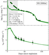 |
Fig. 1. Observed bolometric LC (top panel) and Fe IIλ5169 line velocities (bottom panel) of SN 2006ai (filled markers) with models randomly sampled from the posterior distribution of the parameters (solid lines). The median value and 68% confidence range for every physical parameter are also shown. The grey shaded region shows the early data removed from the fitting (first 30 days after explosion). |
Having inferred the progenitor and explosion properties for a large sample of SNe II (24 SNe in the gold sample and 53 in total), we now analyse the distributions of the physical parameters. This is the largest set of physical properties of SNe II derived to date. For two of the 53 SNe II (SN 2005af and SN 2007it) only MNi was derived. SN 2005af was only observed at late times, from the late recombination phase to the radioactive tail phase. SN 2007it was also observed at late phases and, additionally, it has early observations (< 30 days). These data are insufficient to determine all the physical parameters, and only MNi was inferred.
Figures 2 and 3 display histograms of progenitor (MZAMS, Mej, and R) and explosion parameters (E, MNi, and 56Ni mixing), respectively. In each panel, the yellow bars represent SNe II in the gold sample, while the histogram of the full sample is indicated in red bars. We characterise the distributions by the 16th, 50th, and 84th percentiles. Additionally, Figs. 2 and 3 show the probability density function of the parameters. These functions were computed using a kernel density estimation of the sum of the posterior distributions marginalised over the parameters for the SNe II in the gold (solid lines) and full (dashed lines) samples. We note that some values exceed unity. This is not erroneous since the figure shows the probability density function. The integral of the probability density function along the entire range of values equals unity.
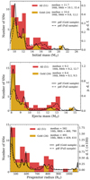 |
Fig. 2. Histograms of three progenitor parameters: MZAMS (top panel), Mej (middle panel), and R (bottom panel). The gold sample is represented by yellow bars, and the red bars are the histograms for the full sample. In each panel, the number of SNe II is listed, together with the median and the 16th and 84th percentiles. Probability density functions of the physical parameters for the gold and full samples are represented by solid and dashed lines, respectively. |
The MZAMS distribution for the SNe II in the gold sample (Fig. 2, top panel) is characterised by a median value of 10.4 M⊙, with most progenitors (21 of 24) being less massive than 13 M⊙. When the full sample is considered the median is slightly larger, MZAMS = 11.7 M⊙. For both the gold and full samples, the lowest and highest MZAMS values are found to be 9.2 and 20.9 M⊙ for SN 2009N and SN 2008ag, respectively. SN 2008ag presents one of the longest and brightest optically thick phases in the sample (Paper I), and thus it is not surprising to find a massive progenitor with large pre-SN mass and radius to reproduce its observations. None of the SNe II in the sample is consistent with explosion models for stars more massive than 21 M⊙. This is in accordance with several studies that analyse SN II progenitors in pre-explosion images, that also find a lack of high-mass RSG progenitors (Smartt 2015; Davies & Beasor 2018). On the other hand, the lower boundary of our MZAMS distribution is consistent with the lowest-MZAMS progenitor model. In Sect. 6.1, a full analysis of the MZAMS distribution is given.
The histograms of Mej (Fig. 2, middle panel) and R (Fig. 2, bottom panel) can be explained from the MZAMS distributions. The Mej and R are not model parameters, and therefore these values were directly inferred from the MZAMS value derived from the fitting. As more low-MZAMS progenitors are recovered, it is expected that most of the SNe II have low Mej and R (under the assumption of standard single-star evolution used in this study). The median Mej is 8.4 M⊙ for the gold sample, and 9.2 M⊙ when all SNe II are analysed. As for the MZAMS, the lowest and highest Mej and R are obtained for SN 2009N and SN 2008ag, respectively (for both gold and full samples). The values of Mej range from 7.9 to 14.8 M⊙, and from 450 to 1077 R⊙ for the pre-explosion radius. The median R is 495 R⊙ for the gold sample, and 582 R⊙ for the full sample.
The top panel of Fig. 3 shows the histograms for the explosion energy. The gold sample ranges from 0.15 foe (SN 2008bk) to 1.25 foe (SN 2006ai) with a median value of 0.61 foe. The full sample spans a larger range of E from 0.15 foe (SN 2008bk) to 1.40 foe (SN 2006bl), with a median value of 0.63 foe. The MNi distribution is displayed in the middle panel of Fig. 3. We could determine the 56Ni mass for 17 SNe II as only these present observations during the radioactive tail. Uncertainties in the explosion epoch, host-galaxy extinction, and distance impact on the determination of MNi. While some SNe II have lower uncertainties in the parameters mentioned above, these SNe are not necessarily the same as those in the gold sample above. Thus, to avoid confusion with the previously defined sub-samples, we did not separate SNe II into different samples for the derivation of their 56Ni masses. The median of the distribution is 0.036 M⊙, and it ranges from 0.006 M⊙ for SN 2008bk, to 0.069 M⊙ for SN 2007X. In Paper I, we found that SN 2008bk is the lowest-luminosity event at the radioactive tail phase, and therefore it is unsurprising that SN 2008bk has the lowest estimated MNi. The bottom panel of Fig. 3 shows the 56Ni mixing distributions. 56Ni mixing values range from the inner ejecta (0.2) to the outer ejecta (0.8) with a median of 0.53 for the gold sample, similar to that for the full sample. Only a few SN II explosions are consistent with extended 56Ni mixing (∼0.8) into the ejecta.
6. Analysis
6.1. The mass function of SN II progenitors
Most studies of the initial mass function (IMF) of SN II progenitors use information from pre-explosion images (e.g. Smartt et al. 2009; Smartt 2015; Davies & Beasor 2018, although see Morozova et al. 2018). A discussion of their results is presented in Sect. 7.1. In the current work, we study the MZAMS distribution of SN II progenitors using the values derived for the CSP-I sample. Restricting ourselves to the gold sample we have 24 MZAMS estimations. This number increases to 51 if we consider the full sample. To date, this is the most homogeneous and largest sample of progenitors of SNe II analysed from hydrodynamical modelling. Our analysis is based on fitting a power law to the inferred MZAMS distribution employing a Monte Carlo (MC) method to randomly sample the masses from a master population. This technique is similar to that presented by Davies & Beasor (2020), where the reader is referred for details.
We first constructed the cumulative distribution (CD) of the MZAMS for the progenitors. We performed 10 000 MC simulations to determine the probability distribution of the CD. For each simulation, MZAMS was randomly sampled from the probability distribution of each progenitor, which was obtained from our MCMC procedure (Sect. 4.2), and then the progenitors were ordered in increasing MZAMS. As noted in Davies & Beasor (2020), when sampling from the posterior distribution, the MZAMS of a progenitor can take different values producing changes in the order of the progenitors. For this reason, it is necessary to re-order the progenitor masses at each MC trial. Figures 4 and 5 show the progenitor masses in increasing order (filled squares) and the confidence regions of the CD of the masses (filled contours) for the gold and full samples, respectively.
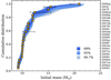 |
Fig. 4. Cumulative distribution of MZAMS for the SN II progenitors in the gold sample. The derived masses are shown in yellow squares. The shaded contours show the confidence regions of the CD. |
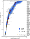 |
Fig. 5. Same as in Fig. 4 but for the SN II progenitors in the full sample. Yellow squares represent the SNe II in the gold sample. |
Then, the CDs derived above (i.e. the shaded contours in Figs. 4 and 5) were fitted with models of CD based on power laws. These models have the following input parameters: the lower and upper MZAMS limits of the distribution (Mlow and Mhigh, respectively), and the slope of the power law (Γ). For each set of parameters, we employed 10 000 MC trials to determine the posterior probability distribution for the model CD of the masses. We found the probability distributions of the parameters via MCMC methods. Results are characterised by the median of the marginal distributions, adopting the 16th and 84th percentiles as the lower and upper uncertainties, with one exception (see below).
In the following, we focus on the analysis of the gold sample. The full sample is analysed later. Figure 6 shows the CD of MZAMS obtained for the gold sample in comparison with the theoretical CD based on power laws. The yellow triangles and error bars represent the median and the 68% confidence level of the distribution presented in Fig. 4 as shaded contours. The shaded regions in Fig. 6 correspond to the theoretical CD constructed with the median values of the marginal distributions of the parameters. As previously indicated, 10 000 MC simulations were performed to construct this theoretical CD. A corner plot of the joint posterior probability distribution of the parameters is presented in the right panel of Fig. 6. We find Mlow = 9.3 M⊙, Mhigh = 24.7
 M⊙, and Γ = −6.35
 . These values are also listed in Table 2. We note that the median value of Mhigh is offset to larger masses from the peak of the distribution, that is, the distribution is skewed to the right. For this reason, we used the mode to characterise the Mhigh distribution and the 68% confidence interval for the uncertainties, finding
  = 21.3
 M⊙. The right-skewed distribution is because of the steepness of the CD of the progenitors. The mass function of SN II progenitors we derive is much steeper than that for a Salpeter massive-star IMF with Γ = −2.35 (Salpeter 1955). With a steep power law of Γ = −6.35 we do not expect high-mass progenitors to be within our sample. The vast majority of the stars are found near the value of Mlow, and changes in Mhigh to larger values do not significantly alter the distribution. For a standard Salpeter IMF, 90% of the stars between 9−25 M⊙ (the range of our pre-SN models) are in the 9−21 M⊙ range. Then, in our sample of 24 progenitors, we would expect to find two progenitors with masses above 21 M⊙. This is not the case for our defined Γ. Not only we do not have progenitors with MZAMS above 21 M⊙, we also find a large number of low-mass progenitors. In the gold sample, 87% of the progenitors have MZAMS < 13 M⊙, while the expected value for a Salpeter IMF is ∼50%.
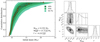 |
Fig. 6. Fits to the CD of MZAMS of SN II progenitors in the gold sample. Left panel: CD of MZAMS derived in our work for the gold sample (yellow triangles and error bars), corresponding to the median and the 68% confidence limit of the distribution presented in Fig. 4 as shaded contours, in comparison with the model CD constructed with the median values of the marginal distributions of the parameters (shaded contours). Right panel: corner plot of the joint posterior probability distribution of the parameters. Dashed lines indicate the 16th, 50th, and 84th percentiles of the distributions. |
Parameters of the cumulative distributions.
Following the above results when leaving the power law as a free parameter, we now compare the CD of MZAMS to models with the power-law slope set to −2.35 (i.e. a standard Salpeter IMF). In this present case, we find Mlow = 8.5 M⊙ and Mhigh = 19.1
 M⊙ (Fig. 7, right panel). The CD model drawn from the posterior distribution of the parameters shows discrepancies with the CD of progenitor masses derived from our modelling (Fig. 7, left panel). The differences are due to the large number of low-MZAMS progenitors found.
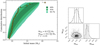 |
Fig. 7. Same as in Fig. 6 but when the power-law slope is fixed to Γ = −2.35, that is, the slope of a Salpeter massive-star IMF. |
The same analysis was performed for the full sample of SN II progenitors. Here, we find the following parameter values: Mlow = 9.3 M⊙, Mhigh = 21.5
 M⊙, and Γ = −4.07
 . In Fig. 8, we show the CD of MZAMS obtained for the full sample (red triangles and error bars corresponding to the median and 68% confidence limit of the distribution presented in Fig. 5 as shaded contours) in comparison with the model CD constructed with the median values of the marginal distributions (shaded contours). In addition, Fig. 8 shows a corner plot of the posterior probability distribution of the parameters. The values of Mlow and Mhigh are similar for both the gold and full samples. The largest differences are found for the power-law slope. This is shallower than that obtained for the gold sample, although it is still steeper than a Salpeter IMF. In Sect. 7.2.1 we analyse whether the different sample sizes influence the power-law slope obtained.
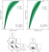 |
Fig. 8. Fits to the CD of MZAMS of SN II progenitors in the full sample. Top left: CD of MZAMS derived in our work for the full sample (red triangles and the error bars), corresponding to the median and the 68% confidence limit of the distribution presented in Fig. 5 as shaded contours, in comparison with the model CD constructed with the median values of the marginal distributions of the parameters (shaded contours). Bottom left: corner plot of the joint posterior probability distribution of the parameters. Dashed lines indicate the 16th, 50th, and 84th percentiles of the distributions. The right panels show the same as the left panels but when the power-law slope is fixed to Γ = −2.35. |
Additionally, we computed the lower and upper mass limits if we constrain Γ = −2.35 (top-right and bottom-right panels of Fig. 8). We find Mlow = 9.0 M⊙ and Mhigh = 19.0
 M⊙. Here, the model drawn from the median values of the parameter distributions can mostly reproduce the behaviour of the MZAMS distribution. At first glance, Mhigh is smaller than the upper mass boundary of the derived cumulative mass distribution (red triangle in the top-right panel of Fig. 8). However, the upper mass boundary has a value of MZAMS = 21.0
 M⊙ (99.7% confidence), that is, they are coincident at the 99.7% significance level. In both the gold and full samples, we find steeper power laws than that of a Salpeter massive-star IMF. In Sect. 7 we discuss possible reasons of this discrepancy, which we term ‘the IMF incompatibility’.
6.2. Ejecta masses and explosion energies
Here we discuss the range of ejecta masses and explosion energies obtained in our work. Figure 9 compares our results to those from other studies involving large samples of SNe II. For this purpose, we used the results published in Utrobin & Chugai (2019), which summarises previous estimates from a series of papers by those authors and the results of Pumo et al. (2017) on under-luminous SNe II. Pumo et al. (2017) also complies the results of several ‘normal’ SNe II obtained with the same code. We also compare with the ejecta masses and explosion energies from Ricks & Dwarkadas (2019). All the above-mentioned studies present detailed modelling of LCs and expansion velocities for several SNe II. Morozova et al. (2018) presented LC modelling for 20 SNe II. Given that our distributions were derived from the modelling of the LC and expansion velocities simultaneously, a direct comparison is difficult. However, we include the results from Morozova et al. (2018) in the comparison. Unfortunately, we cannot compare with the findings from Eldridge et al. (2019) as only the initial masses were published.
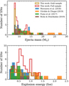 |
Fig. 9. Comparison of ejecta masses (top panel) and explosion energies (bottom panel) derived in the current work to those from previous studies containing large samples of SNe II. |
We observe that our Mej and E are generally consistent with those from previous studies as our results fall within the range of previous estimates. However, we note a spike at ∼8−9 M⊙ that is not found in the other studies8. This spike is the reason why we found so many low-MZAMS progenitors, causing the IMF incompatibility (see Sect. 7.2).
The highest estimated Mej and E for the CSP-I SN II sample are 14.8 M⊙ and 1.25 foe (1.40 foe for the full sample), respectively. A number of higher Mej and E are found in the other works, especially in those from Utrobin & Chugai (2019). This could be because these authors use non-evolutionary models as pre-SN configurations that are capable of producing a large variety of pre-explosion structures, each with different mass, radius, chemical composition, and density profile. In the present work, we used standard single-star evolution calculations as pre-SN models. Therefore, the initial density profiles were not freely chosen, and the range of pre-SN parameters is confined. In our set of progenitor models, the highest Mej is 15.7 M⊙, coming from a 24 M⊙ progenitor in the ZAMS (see M20, their Fig. 2). Therefore, it is impossible for us to find larger Mej given that we only consider MZAMS up to 25 M⊙. Ricks & Dwarkadas (2019) obtained a Mej of ∼20 M⊙ for SN 2015ba using evolutionary models to initialise the explosion. However, for this particular progenitor model, the authors used a lower scaling factor for the efficiency of mass loss via winds during the stellar evolution producing a more massive star at explosion time. We again stress that our pre-SN models were calculated using the standard assumptions and parameters during the evolution. Different stellar evolution assumptions can lead to different results.
Pumo et al. (2017) found, on average, lower Mej and E than other studies probably because most of their sample corresponds to low-luminosity SNe II. While the range of parameters found is in good agreement with that from Morozova et al. (2018), we find some differences in the distributions. Morozova et al. (2018) found more SNe II with lower energies, while at the same time, a spike at Mej ∼ 14 M⊙.
Finally, we compare the explosion energies in this work with those expected from neutrino-driven explosion models. 1D core-collapse models found explosion energies ranging from 0.1 to 2.0 foe (Ugliano et al. 2012; Ertl et al. 2016; Sukhbold et al. 2016). The SNe II modelled in this work do not cover the entire range of explosion energies predicted by the explosion models, particularly because our maximum value is somewhat lower (1.25 foe for the gold sample and 1.40 foe for the full sample). More energetic explosions produce more luminous SNe II, which are not found in our sample. For example, the highest explosion energies found in Sukhbold et al. (2016) produce plateau luminosities higher than 1042.6 erg s−1 (see their Fig. 31), while in the CSP-I SN II sample, only one object – SN 2009aj – has plateau luminosities above this value. In addition, as previously discussed in Sect. 5, SN 2009aj may be powered by interaction between the ejecta and a massive CSM. More recently, Burrows et al. (2020) conducted 3D core-collapse simulations in a wide range of progenitor masses. The lowest-MZAMS model (9 M⊙) in their grid achieves an explosion energy of ∼0.1 foe, which is compatible with the lowest explosion energy found in our study. Unfortunately, the other core-collapse models have not reached the asymptotic explosion energy by the end of the simulations. However, these authors do find that progenitors with higher MZAMS attain higher explosion energies. We find the same trend in Paper III.
6.3. Progenitor radii
Levesque et al. (2005, 2006) studied Galactic and Magellanic Cloud RSGs and obtained their radii using the Stefan-Boltzman law from effective temperatures and bolometric luminosities. These studies found that most RSGs have radii between 100 and 1500 R⊙. In Sect. 5, most progenitor radii inferred from our LC and velocity modelling are found within the range of 450−600 R⊙. However, we emphasise that progenitor radius is not an independent parameter in our modelling. Our fitting routine derives MZAMS, which relates to pre-SN structures with different characteristics (e.g. ejecta mass, radius, among other physical parameters). Additionally, while early-time optical LCs are most sensitive to progenitor radius, in the current work fits were performed only to observations later than 30 days from explosion (see Sect. 4.3).
6.4. 56Ni masses
The 56Ni masses for the CSP-I SN II sample range from 0.006 M⊙ through 0.069 M⊙ with a median of 0.036 M⊙. Our values were determined for 17 SNe II which do not cover the entire 56Ni mass range found in the literature. Some SNe II have been found with more and less 56Ni (e.g. Hamuy 2003; Pastorello et al. 2004; Pumo & Zampieri 2011). MNi was estimated for all CSP-I SNe II with bolometric data during the radioactive tail phase9, suggesting that the MNi range of our models (see Table 1) was sufficient and the inclusion of models with MNi larger than 0.08 M⊙ into our grid of simulations was not necessary.
Pejcha & Prieto (2015) estimated MNi for 21 SNe II and found a minimum of 0.0045 ± 0.0008 M⊙ for SN 2001dc10 and a median of 0.030 M⊙. Both the median and minimum values are consistent with our determination. However, a large discrepancy is found for the maximum value. Pejcha & Prieto (2015) inferred a 56Ni mass yield of 0.28 M⊙ for SN 1992H, which is significantly higher than the 0.069 M⊙ estimated in our study for SN 2007X. Pejcha & Prieto (2015) inferred a larger distance to SN 1992H than previous estimates (Schmidt et al. 1994; Clocchiatti et al. 1996) making this SN more luminous compared to normal SNe II, and therefore, with a larger MNi.
Müller et al. (2017) determined MNi for 19 SNe II and combined their sample with that from Pejcha & Prieto (2015) making a larger sample of 38 objects. Their MNi distribution is described by a median value of 0.031 M⊙ – consistent with ours – with values between 0.005 and 0.280 M⊙. The latter value corresponds to SN 1992H as described above. More recently, from a compilation of 115 SN II 56Ni mass estimates from the literature, Anderson (2019) estimated a median value of 0.032 M⊙, in agreement with our results. The minimum and maximum values in Anderson (2019) are 0.001 and 0.360 M⊙, respectively. This range is larger than that determined in our study, particularly because the high 56Ni mass estimate of 0.360 M⊙ (for SN 1992am; Nadyozhin 2003) is significantly larger than the maximum value estimated for the CSP-I sample. The larger sample in Anderson (2019) may indicate that values above the adopted maximum in our models of 0.08 M⊙ are exceptional. Around 10% of the SNe II in the literature have estimated 56Ni masses above 0.08 M⊙ (see Fig. 1 from Anderson 2019). However, some of these SNe II are classified as 1987A-like events, which have relatively high 56Ni masses compared to the ‘normal’ SNe II studied in the current work. Additionally, a few SNe II have more than one 56Ni mass estimate in the literature, and some of these are consistent with our adopted maximum 56Ni mass. Differences are attributed to distinct distance and reddening values used in the literature for the same SN.
Sukhbold et al. (2016) report 56Ni masses based on neutrino-powered explosions for numerous pre-SN models within a large range of initial masses. The minimum MNi values in Sukhbold et al. (2016) are 0.003 and 0.006 M⊙ for the 9.25 and 9.0 M⊙ models, respectively. The different values correspond to the different codes used for their calculation. These values are similar to the lowest MNi derived for our SN II sample. For stars between 10 and 25 M⊙ (the maximum initial mass in our pre-SN models), most MNi values are found within the range of 0.01−0.08 M⊙, which is consistent with our findings. Only a few explosion models produce larger MNi in Sukhbold et al. (2016), with a maximum value of ∼0.10 M⊙.
6.5. 56Ni mixing
During a SN explosion, a shock wave emerges heating the stellar material. If the shock temperature is sufficiently high, explosive nucleosynthesis takes place. Explosive nucleosynthesis efficiently produces heavy elements from Si to Zn (Umeda & Nomoto 2002). 56Ni dominates the production of nuclear species in the inner regions of the star, but Co, Zn, and additional Ni isotopes are also mostly produced here (Woosley & Weaver 1995; Thielemann et al. 1996; Umeda & Nomoto 2002). Once the shock reaches the composition interfaces between the carbon-oxygen core and the helium core, and the helium core and the hydrogen-rich envelope, RT instabilities appear causing a large-scale spatial mixing. This is the mechanism by which the heavy elements synthesised during explosive burning can reach the outer regions of the envelope while hydrogen can be mixed inwards.
The first evidence of chemical mixing during the explosion was based on the observations of SN 1987A. A substantial amount of 56Ni mixed into the hydrogen-rich envelope is required to explain the rise time to peak of SN 1987A (Shigeyama et al. 1988; Shigeyama & Nomoto 1990), and the LC and spectral evolution of X-rays and γ-rays (Kumagai et al. 1989). Furthermore, the presence of significant Fe emission at high velocities during the nebular phase demonstrates that a significant amount of 56Ni was mixed into the hydrogen-rich envelope during the explosion (Haas et al. 1990). While the progenitor of SN 1987A is a blue supergiant (BSG) star, SN II progenitors are known to be RSGs with significantly distinct pre-SN structures. Recent 3D hydrodynamical simulations of the evolution of the SN shock for both BSG and RSG explosions have shown that RSG models achieve higher maximum velocities for the 56Ni into the ejecta (Wongwathanarat et al. 2015) implying more extended mixing of 56Ni.
In Sect. 5 we showed that the 56Ni distribution in the ejecta covers the range of initial values, from 0.2 (inner ejecta) to 0.8 (outer ejecta). However, in both the gold and full samples, the vast majority of the events are found within low (0.2−0.4) and moderate (0.4−0.6) values and only a low number of SNe II are found with a large extent of 56Ni mixing (Fig. 3, bottom panel). An extreme mixing of 56Ni is hard to obtain in RSGs because of their large envelopes. Our results are consistent with this concept given that an extended 56Ni mixing was only found for one SN II in the gold sample (SN 2008ag, 56Ni mixing = 0.8). We note that the 56Ni mixing is characterised as a fraction of the pre-SN mass. This means that the same value of 56Ni mixing for different progenitors may represent different extents of 56Ni in mass and radial coordinates.
We stress that in this study the 56Ni mixing is treated as a free parameter. Recently, Wongwathanarat et al. (2015) computed 3D hydrodynamical simulations and found that the extent of the mixing of the metal-rich ejecta depends on the early-time asymmetries generated by the neutrino-driven mechanism, explosion energy, and progenitor structure. In the progenitor structure, the most important features are the width of the carbon-oxygen core, the density structure of the helium core, and the density gradient at the composition interface between the helium core and hydrogen-rich envelope. However, only a few hydrodynamical simulations for RSG models have been carried out in the literature. Further studies are crucial for better understanding of the 56Ni mixing process in SNe II.
6.6. Explosion epochs
We compared the explosion epochs derived in our analysis with those from Gutiérrez et al. (2017b) for each SN. Our estimations are always inside the range of values derived by Gutiérrez et al. (2017b), which is by design since we did not allow our fitting procedure to sample values outside that range (see Sect. 4.2). The mean difference between both estimates is 0.1 days with a standard deviation of 4.8 days. There are a few cases where our explosion epoch estimates are very close to the observational limits, possibly suggesting explosion dates beyond the uncertainties of Gutiérrez et al. (2017b). In M20, we tested this by relaxing the prior for the explosion epoch and obtained a similar marginal distribution of the physical parameters, indicating no changes in our results.
That the mean offset is so close to zero gives significant support to both methodologies of estimating the explosion epoch. While we did not allow our modelling estimates to be outside the range of the observational errors, the modelling explosion epochs could have been biased towards – on average – higher or lower values than the observational values. In the case of observational explosion epochs, the constraints from the non-detection that the SN has not exploded at that date are only as strong as the survey depth providing the non detection. One could therefore imagine that ‘true’ explosion epochs could be biased towards values close to the non detection. However, the above analysis shows this not to be the case, and therefore gives support to the observation epochs as estimated by Gutiérrez et al. (2017b). At the same time, one could imagine that a bias in the modelling technique could mean that the fitting could attempt to use the prior on the explosion epoch to systematically offset the plateau duration – and therefore the ejecta mass – to lower or higher values by constraining the explosion epoch to be later or earlier, respectively (with respect to the observational value). Again, this is not seen in our data, giving support to the robustness of our model fitting methods.
6.7. Non-standard SNe II
In this study, we utilise a large grid of explosion models assuming standard values for several stellar evolution parameters (metallicity, wind efficiency, mixing length, and overshooting) and explosion parameters (M20). Although most of the well-sampled SNe II in the CSP-I sample can be adequately reproduced by the models in this grid, some are not.
SN 2006Y and SN 2008bu reside in the lower end of the optically thick phase duration distribution with 64 ± 4 days and 52 ± 7 days, respectively (Paper I). Unfortunately, no model in our grid has such a short optd. In the case of SN 2006Y, the closest fitting models can reproduce the velocities and the plateau luminosity reasonably well. However, the optd is overestimated by ∼10 days. At first sight, this difference is small, but the models also largely underestimate the radioactive tail luminosity by ∼0.6 dex. Additional 56Ni can easily fit the tail, but it is known that more 56Ni also produces a longer plateau phase (e.g. Kasen & Woosley 2009; Bersten 2013), which increases the discrepancy with the observations. On the other hand, for SN 2008bu, the situation is even worse as the optd lasts ∼10 days less than that of SN 2006Y.
Theoretical studies suggest that progenitors with smaller hydrogen-rich envelope masses at time of collapse produce shorter optd (e.g. Litvinova & Nadezhin 1983; Kasen & Woosley 2009; Bersten 2013). Following the standard mass-loss rate in the stellar modelling of single stars (as we assume in this study) it is not possible to find such stripped progenitors with MZAMS smaller than 25 M⊙, which is the highest-mass progenitor in our grid. More massive stars can finish with smaller envelopes but they are more difficult to explode (Sukhbold & Adams 2020). Therefore, lower ejecta masses can be achieved by increasing the mass-loss rate via stellar winds, interacting binaries, or rotation, among other possibilities (as discussed in Sect. 7). We calculated new pre-SN models with enhanced mass loss providing much better fits to SN 2006Y and SN 2008bu. These results are presented in Paper III. Our results agree with those from Hiramatsu et al. (2021). These authors presented models for SN 2006Y, as well as other two short-plateau SNe II, from high-mass progenitors that experience more mass loss than standard stellar evolution.
SN 2004er also shows some discrepancies between models and observations, especially with the velocities. SN 2004er shows the longest optd with 146 ± 2 days (Paper I). Its bolometric LC is mostly well-reproduced with the exception that the fitting models show shorter optd by ∼10 days. The largest discrepancy is found in the velocity evolution, where the observed Fe II velocities are greater than the models by ∼2000 km s−1. In fact, SN 2004er displays higher Fe II velocities than most SNe II. For example, the Fe II velocity at 55 days post-explosion is 5033 ± 751 km s−1, while the mean Fe II velocity of SNe II at 53 days is 3537 ± 851 km s−1 (Gutiérrez et al. 2017b). Such large velocities can be achieved through higher explosion energies, although this would produce more luminous and shorter plateau phases. However, larger ejecta masses have the opposite effect, that is, dimmer SNe II with longer plateaus. Therefore, SN 2004er was probably a high-energy explosion of a star with a massive pre-SN envelope – a model that is beyond the parameter space sampled in the current study (and therefore beyond stellar evolution with standard assumptions and/or values of the input parameters). Something similar happens for SN 2007sq. Its bolometric LC is well fit by our standard models, but our model velocities fall below observations. The SNe II above analysed (SNe 2004er, 2006Y, 2007sq, and 2008bu) may be examples of high-mass RSG progenitors that could explain the lack of more massive progenitors in the sample, although a detailed analysis is necessary.
Finally, we briefly describe the fitting models of SN 2008K. These models show offsets both in the bolometric LC and velocities with respect to the observations. The bolometric LC is well fit in general, but when looking at the details, it is seen that the models do not resemble the linear behaviour of SN 2008K, which has a plateau decline rate of 1.70 ± 0.31 mag per 100 days (Paper I). SN 2008K also has higher Fe II velocities than most SNe II. In principle, more energy is needed to reproduce the velocities. This implies more mass to conserve the plateau duration (more energy reduces the plateau length). However, we compared SN 2008K with higher-energy and more-massive explosion models and found even larger discrepancies given that the new parameters produce LCs similar to typical SNe IIP. The detailed pre-SN and explosion properties of SN 2008K are still uncertain. The examples above reflect that some of the standard assumptions in stellar evolution cannot cover all the physical properties of SN II progenitors. Non-standard stellar evolution is required to explain the properties of some individual SNe II.
7. Discussion
7.1. The RSG problem
During recent years, the number of works studying the MZAMS distribution of SN II progenitors has increased. Smartt et al. (2009) were the first to analyse the MZAMS distribution from observed progenitors in pre-explosion images, founding a maximum MZAMS of 16.5 ± 1.5 M⊙. This is in contrast with model predictions and that more massive RSGs are observed in the Local Group (Levesque et al. 2006; Neugent et al. 2020). The lack of higher-mass progenitors is called the ‘RSG problem’. Since then, special attention has been given to the upper mass boundary of the MZAMS distribution. This limit is crucial to understanding the evolutionary pathways of massive stars. A larger set of SN II progenitors consisting in 13 detections and the same number of upper limits was studied by Smartt (2015), but no progenitors were found with MZAMS above 18 M⊙.
Inferring the progenitor MZAMS from a direct detection requires a previous estimation of the progenitor luminosity. This is used to compare with the luminosity predicted by stellar evolution theory. Thus, the physical models provide an estimate of the mass from a luminosity measurement. In this context, Straniero et al. (2019) studied the role of convection, rotation, and binarity in SN II progenitor evolution finding that neither of these uncertain processes in stellar modelling can mitigate the RSG problem.
The progenitor luminosity can be achieved by fits to the spectral energy distribution if the progenitor is detected in several bands, or by using bolometric corrections to convert single-band flux into luminosity. The uncertainties in the latter case may be large if only single-band or two-band detections are available. Davies & Beasor (2018) investigated this source of systematic error and derived new bolometric corrections and extinction values. Those authors found an increased upper mass limit of Mhigh = 19 (68% confidence), with a 95% upper confidence limit of < 27 M⊙. Additionally, Davies & Beasor (2018) analysed the effects of a small sample size on Mhigh, concluding that this causes a systematic error of ∼2 M⊙ that shifts the upper mass limit to larger values. Recently, Davies & Beasor (2020) inferred the properties of the progenitor distribution but working directly with the observed luminosities, thus eliminating the uncertainties introduced in stellar modelling when converting the observed luminosities into MZAMS. Finally, they compared their maximum luminosity with stellar models and found a Mhigh of 18−20 M⊙. However, they remark that the sample size should be at least doubled to enable a reduction in the large uncertainties on Mhigh.
The direct detection of progenitors in pre-explosion images is the most powerful tool to determine the nature of progenitor stars as it can be directly linked to a progenitor system. However, the analysis of direct detections can only be applied – when pre-SN images exist – to the nearest SNe (d ≲ 30 Mpc) due to the lack of resolution for more distant objects. The study of the stellar populations in the immediate SN environments is an alternative indirect method that is also useful for nearby objects where individual stars or clusters are resolved. This information can yield constraints on the ages, and therefore, on the progenitor masses. These measurements are mostly consistent with initial masses of SN II progenitors lower than 20 M⊙, although they present larger uncertainties than the direct identification of the progenitor star (e.g. Van Dyk et al. 1999; Williams et al. 2014; Maund 2017).
Nebular spectra can also be used to constrain the progenitor mass. After the optically thick phase, when all the hydrogen is recombined, the core of the progenitor star becomes visible and nucleosynthesis yields can be analysed (Jerkstrand et al. 2012; Dessart & Hillier 2020). Using this method, most of the mass estimates agree with the lack of high-mass progenitors (see e.g. Jerkstrand et al. 2014; Valenti et al. 2016). However, Anderson et al. (2018) infer an initial mass of 17−25 M⊙ for SN 2015bs through comparison to nebular-phase spectral models suggesting an explosion of a higher-mass progenitor than previously observed for a SN II.
Different alternatives have been proposed to solve the RSG problem. One possibility is that high-mass progenitors do not explode and instead collapse into black holes. Massive stars in the range of the missing RSG progenitors could have pre-SN core structures that are generally more difficult to explode (see e.g. O’Connor & Ott 2011; Sukhbold & Adams 2020). The search for failed SNe has found possible candidates corresponding to high-mass stars (Adams et al. 2017; Allan et al. 2020; Neustadt et al. 2021), lending support to theoretical predictions. In addition, it has been suggested that more massive RSGs produce weak explosions leading to faint SNe II (Fryer 1999; Heger et al. 2003). Zampieri et al. (2003) investigated the possibility that two low-luminosity SNe II (SN 1997D and SN 1999br) could be produced in low-energy explosions of massive progenitors. An alternative solution posits that stellar evolution models could be modified in order to increase the mass loss and reduce the maximum theoretical mass of stars exploding as a RSG. With this assumption, massive stars in the range of the missing RSG progenitors will explode as stripped-envelope SNe instead of SN II events (see e.g. Yoon & Cantiello 2010; Ekström et al. 2012).
Unfortunately, most of the previously mentioned methods to constrain progenitor parameters of SNe are restricted to nearby events because they require either images of high enough resolution and sensitivity or spectra at late-time epochs when the SN is significantly dim. Hydrodynamical modelling of LCs (and sometimes spectra) is one of the most commonly applied indirect methods to infer physical properties of SNe II as it can be applied to large distances, and therefore statistically significant samples. Morozova et al. (2018) inferred progenitor and explosion properties of a sample of 20 SNe II from LC modelling and used the derived MZAMS to explore the mass distribution. They found an upper mass cut-off of Mhigh = 22.9 M⊙ (∼30 M⊙ at 95% confidence limit). However, Morozova et al. (2018) did not consider expansion velocities in their modelling, the exclusion of which has been shown to bias progenitor masses to larger values (see M20).
In Sect. 6.1 we determined the IMF parameters (Mlow, Mhigh, and Γ) for the gold and full samples. For each sample, we also fitted the IMF leaving Γ as a free parameter or fixing it to −2.35. Thus, in total, we have four different estimations of the IMF parameters. All these estimations find Mhigh ≲ 21.5 M⊙. In principle, this is consistent with the RSG problem. However, different levels of significance are found for each estimation, which are examined below. We first analyse the cases when Γ is left as a free parameter. We find Mhigh = 21.3 M⊙ for the gold sample, that is, Mhigh = 25 M⊙ is within the 68% confidence limit. The study of the full sample indicates Mhigh = 21.5
 M⊙ (68% confidence) with a 95% upper confidence limit of < 27.1 M⊙. While this increases the significance of our results with respect to the RSG problem, we note that the results obtained from the full sample are not as robust as those from the gold sample. When Γ is fixed to the value of a Salpeter massive-star IMF, we find Mhigh < 21 M⊙ for both the gold and full samples. In these two cases, the RSG problem is recovered with a significance above the 99% significance level.
7.2. The IMF incompatibility
The SN II progenitor IMF derived in Sect. 6.1 is inconsistent with a Salpeter IMF due to the large difference found in the slope of the distributions – which we named the IMF incompatibility. However, the massive-star IMF is very well established. Several studies of OB associations and clusters suggest that the majority of the stars above a few solar masses are drawn from a Salpeter power-law (Bastian et al. 2010). In addition, progenitor mass constraints from the stellar populations surrounding a SN event and SN II progenitor mass estimations from pre-SN imaging are also drawn from a Salpeter IMF (Smartt 2015; Koplitz et al. 2021). The apparent incompatibility of our results with a standard IMF is driven by the large number of low-MZAMS progenitors found with respect to more massive progenitors. In Sect. 3 we pointed out that CSP-I built a magnitude-limited sample of SNe II. The luminosity function of a magnitude-limited distribution could be biased against lower-luminosity events that generally come from low-MZAMS progenitors and low-energy explosions (see Paper III). This is the opposite of the volume-limited sample of SNe II with progenitor detection in pre-explosion images (Smartt et al. 2009). Given that most SNe II in our sample are consistent with such low-mass events, there does not seem to be significant evidence that this bias is affecting our results or conclusions. We therefore believe that this incompatibility reflects a lack of understanding of some physical ingredients in our study or the completeness of our sample. Here we discuss possible reasons, but a deep and systematic analysis should be carried out in order to identify the ultimate reason for the IMF incompatibility.
7.2.1. Sample size
First, we explore if the IMF incompatibility is consequence of the sample size. We performed a test similar to that presented in Sect. 6.1 for different sample sizes (N). We randomly sampled the initial masses of N progenitors assuming a Salpeter massive-star IMF with Mlow = 9 M⊙ and Mhigh = 25 M⊙ (the MZAMS range of our pre-SN models), and ordered the progenitors in increasing mass. We performed 10 000 MC simulations to determine the CD of the masses for each value of N, and then we fit power-law models to these CDs. Given that we are interested in testing the sample size effect in the estimation of Γ, we constrained Mlow and Mhigh to 9 and 25 M⊙, respectively, which means that Γ was the only parameter to determine. The posterior distribution of the Γ parameter was found via an MCMC procedure. We employed 10 000 MC trials to determine the posterior probability distribution for the progenitors at each Γ value. We performed the same experiment for a range of sample sizes.
The results of this test are presented in Fig. 10. The larger the sample size, the best-fitting Γ tends to the value of the Salpeter IMF slope (−2.35, black solid line). For 24 objects (i.e. the number of SNe II in the gold sample), the best-fitting Γ is −2.50 , which means that Γ = −2.35 is within the 68% confidence interval. Something similar happens for N = 51 (i.e. the number of SNe II in the full sample with MZAMS estimates), where we find −2.45
 . This indicates that our sample size do not produce the bias we found in the IMF. As the IMF incompatibility cannot be explained by the sample size, in the following sections we discuss some possible physical reasons for this discrepancy.
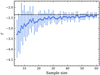 |
Fig. 10. Best-fitting power-law slope of the CD of the progenitor masses for a range of sample sizes. The error bars correspond to the 68% confidence limit. The larger the sample, the higher the probability that the best-fitting power-law slope is that of a Salpeter IMF. The solid black line indicates the Salpeter IMF slope for massive stars. |
From Fig. 10, we also note the best-fitting Γ differs significantly from that of a Salpeter IMF for samples smaller than 20 objects. This restricts future studies to work with larger samples for a reliable estimate of the power-law slope.
7.2.2. Pre-SN models
The IMF incompatibility is produced by the large relative number of low- to high-MZAMS progenitors. In Sect. 5 we found a large number of explosions with progenitor structures compatible with Mej in the range of 8−10 M⊙ and R between 450 and 650 R⊙ (Fig. 2, middle and bottom panels). In the context of standard single-star evolution adopted in the current study, these pre-SN structures are consistent with low-MZAMS progenitors. However, if the standard assumptions in stellar evolution change (which is possible given the uncertainties in massive-star modelling), different pre-SN configurations could be obtained for the same MZAMS value. Below we discuss how different factors such as the envelope stripping processes, metallicity, mixing length, and overshooting can affect the pre-SN structure, and therefore our results.
Mass-loss rate. Similar Mej (for higher MZAMS) can be achieved by increasing the mass-loss rate via stellar winds, eruptive mass-loss events, rotation, binary interaction, or a combination of these phenomena. If more mass were lost by progenitors, then the estimated Mej could be reduced for more massive MZAMS, and thus this would reduce the inconsistency of our results with a standard IMF. While higher mass loss may change the MZAMS distribution derived from hydrodynamical modelling, additional mass stripping does not change the progenitor MZAMS estimations from pre-SN imaging. This is because the progenitor final luminosity is closely related to its helium core mass and it is almost independent of the final envelope mass (direct progenitor observations do not provide ejecta mass estimates). The sensitivity of the initial mass–final luminosity relationship on the adopted mass-loss rate is small (Straniero et al. 2019; Farrell et al. 2020).
Recent studies infer that most massive stars have rotational velocities in the range of 0−300 km s−1 (Ramírez-Agudelo et al. 2013; Dufton et al. 2013). Since rotation increases mass loss, the final mass of rotating stars is smaller than that of non-rotating stars (Hirschi et al. 2004). Following this, if we consider pre-SN models of rotating massive stars we could find lower-Mej for higher-MZAMS progenitors, that is, in the direction to explain the IMF incompatibility.
Beasor et al. (2020) and Humphreys et al. (2020) derived new mass-loss prescriptions based on direct measurements and did not find larger mass-loss rates in the RSG phase than previous estimations. In addition, Beasor et al. (2020) conclude that quiescent mass-loss during the RSG phase (when most of the mass loss occurs) has little effect in stripping the envelope. In principle, this excludes the RSG winds as a mechanism to strip a larger part of the hydrogen-rich envelope (see also Beasor et al. 2021). However, Ekström et al. (2012) proposed new mass-loss prescriptions for RSGs considering that they may undergo episodic mass-loss events (i.e. more mass is lost). Neugent et al. (2020) compared the observed luminosity function of RSGs in M31 to that predicted by the stellar models from Ekström et al. (2012) and concluded that the new prescription for RSG mass-loss rate reproduces the observations. Given the inconsistencies in previous estimations, it is not clear whether mass-loss processes on isolated RSGs are responsible for stripping a significant part of the envelope.
Very early spectra have shown the presence of CSM around SN II progenitors (e.g. Khazov et al. 2016; Yaron et al. 2017; Bruch et al. 2021) indicating that enhanced mass loss might occur prior to core collapse. This is also inferred from early-time LC modelling (e.g. Morozova et al. 2018; Förster et al. 2018). Such high mass-loss rates are not consistent with direct measurements of RSG winds possibly implying another mechanism to induce mass loss. Fuller (2017) suggests that pre-SN outbursts via waves driven by convection during the late stages of evolution may reproduce the CSM properties. However, despite early-time observations of many SNe II indicate very high mass-loss rates shortly before the explosion, the amount of mass involved is small, which means that this process cannot explain the low pre-SN masses.
An efficient way to remove a large fraction of (if not all) the outer envelope of massive stars is through mass transfer to a companion star in a binary system (e.g. Podsiadlowski et al. 1992; Benvenuto et al. 2013). Therefore, this mechanism can produce SN II events with lower ejecta masses than predicted by single-star evolution. According to recent studies, most massive stars belong to binary systems (or higher-order multiples; Moe & Di Stefano 2017). Moreover, it has been shown that a large fraction of massive stars will exchange mass with a companion prior to the RSG phase (Sana et al. 2012, 2013). Recently, from analytical estimations and population synthesis simulations, Zapartas et al. (2019) showed that a large fraction (from one-third to half) of SN II progenitors will interact with a companion star during its evolution. Additionally, Eldridge et al. (2018) showed that the diversity of CCSN LCs can be interpreted as the result of binary interaction. Previously, it has generally been assumed that SN II arise from progenitors that explode with most of their hydrogen envelopes intact. SN II modelling assuming such progenitors has generally been consistent with observations and thus it has not been necessary to invoke binarity. However, this does not mean that the effects of binary evolution are unimportant in explaining SN II observations and diversity. Our results and the above mentioned studies support the hypothesis that many SN II progenitors may experience larger mass loss than expected assuming standard single-star evolution. In addition, a different treatment of mass loss is required in the cases of SN 2006Y and SN 2008bu (see Sect. 6.7 and Paper III). Thus, it may well be that binarity plays a larger role in shaping SN II behaviour than previously assumed. We now discuss whether other stellar parameters can explain the discrepancy.
Metallicity. The influence of metallicity on the winds of hot-massive stars is well known (Vink et al. 2001). However, for single-massive stars, most of the mass lost happens in the RSG phase, where the rate of mass loss is assumed to be nearly independent of metallicity (van Loon 2006; Goldman et al. 2017) at least within the metallicity range of the CSP-I SN II sample (see below). The influence of metallicity on the winds can change the pre-SN structure at the time of collapse. Lower metallicities produce more compact and more massive progenitors (Dessart et al. 2013). However, we do not expect large variations in the metallicity of the CSP-I sample. Anderson et al. (2016) inferred environment metallicities for the CSP-I SN II sample and found a narrow range in metallicities, which is not expected to significantly alter the stellar evolution. In addition, Anderson et al. (2016) found that there is no relationship between progenitor metallicity and SN II LC and spectral properties (except for the metal line equivalent widths). Gutiérrez et al. (2018) also concluded that the hydrogen-rich envelope mass and the explosion energy are not correlated with the metallicity. Therefore, we do not expect that metallicity significantly modifies our results obtained from solar-metallicity stellar models.
Mixing-length parameter. Pre-SN models with different mixing-length parameters differ primarily in the final radius (larger mixing-length parameters produce smaller radii). In our study, we find that most SN II progenitors are consistent with RSG radii between 450 and 600 R⊙ (Fig. 2, bottom panel). The minimum progenitor radius in our grid of pre-SN models is 450 R⊙ (using a mixing-length parameter of two). Smaller radii can be obtained with a mixing-length parameter of three, as previously suggested by Dessart et al. (2013) based on the analysis on SN 1999em. Adopting a larger mixing-length parameter, we would obtain pre-SN structures with similar pre-SN masses but smaller radii. A smaller pre-SN radius for the same initial mass might help to solve the IMF incompatibility as more massive progenitors are needed to derive our radius distribution. However, a direct comparison is not possible given that larger MZAMS progenitors also imply larger ejecta masses and the LC models will dramatically change. Therefore, it would be necessary to carry out a series of simulations before being able to conclude whether or not changes in this parameter could be a determining factor in the IMF incompatibility.
Overshooting. A more extended convective zone produces a more massive helium core, and therefore, higher luminosities. Because of the higher luminosity, the mass-loss rate is larger producing smaller final hydrogen-rich envelope masses. In principle, this can help to solve the discrepancy, but larger overshooting parameters produce much more extended RSGs with dense envelopes (Wagle et al. 2020), acting in the opposite direction to our results. A detailed future analysis should be carried out to fully understand these effects.
7.2.3. Failed SNe II
In the previous sections, we give possible explanations for the IMF incompatibility, but always assuming that the mass function of SN II progenitors should be consistent with a Salpeter massive-star IMF. However, these two distributions may be intrinsically different. Here, we test whether the lack of massive progenitors might be caused by high-MZAMS progenitors failing to produce a SN explosion, where their collapse leads to an implosion into a black hole. If the shock produced by the core collapse fails to explode the RSG star, it may produce a low-luminosity red transient lasting for about a year (Lovegrove & Woosley 2013). Such weak explosions would be difficult to detect and may contribute to the lack of high-MZAMS progenitors.
We constructed a SN II progenitor IMF using the results from Sukhbold et al. (2016), where the authors calculated explosion models for a large and fine grid of pre-SN models and distinguish between exploding and non-exploding cases. The procedure is similar to that presented in Sect. 6.1, but with one exception. Here, at each MC simulation, we randomly sampled a certain number of stars in the range from 9 to 25 M⊙ (the lower and upper MZAMS of our pre-SN models) assuming a Salpeter massive-star IMF with the condition that the sample has 24 objects (i.e. the number of SNe II in the gold sample) after removing the non-exploding stars. We determined the probability distribution of the CD of the MZAMS for the SN II progenitors. We fitted this CD in the same manner as in Sect. 6.1 and found the following parameters: Mlow = 9.1 M⊙, Mhigh = 20.8
 M⊙, and Γ = −3.32
 . These results imply that if failed SNe II are taken into account, the upper MZAMS limit and the slope of the SN II progenitor IMF are modified. A steeper power-law than that of a Salpeter IMF is found, although not as steep as the slope inferred for the gold sample. In addition, for the case of Mhigh, a lower value than that assumed for the Salpeter IMF is obtained.
7.2.4. Modelling
Here we briefly discuss if the differences found in the IMF can be attributed to the simplifications in our hydrodynamical simulations, or to a bias in our fitting procedure.
Hydrodynamical simulations. While the details of the explosion mechanism are still under debate (see Burrows et al. 2020, for a recent review), observations (polarisation, SN remnants, and nebular spectroscopy) show that the explosion is asymmetric in the inner regions (e.g. Hoflich 1991; DeLaney et al. 2010; Taubenberger et al. 2009; Tanaka et al. 2012). However, our hydrodynamic code assumes spherically symmetric explosions, which might produce systematic effects (that would be inherent to all 1D codes).
In our explosion models, the explosion energy is deposited at the inner layers by artificially adding internal energy in form of a thermal bomb. The explosion energy is used to overcome gravity and lifts the envelope out of its potential. The high initial explosion energy produces a strong shock front and pushes the material above resulting in the ejection of the envelope. Inner low-velocity and low-density regions expanding with a certain minimum velocity appear. However, such regions are artefacts of the 1D nature of the modelling. In a spherical explosion, a hot low-density and fast region below a cold and denser stellar structure is formed. Thus, this region is highly RT unstable, with instabilities growing on timescales of seconds to minutes (Janka & Müller 1993). In multi-dimensional calculations, RT instabilities mix material filling the inner low-density region. The inner low-density and low-velocity region present in 1D codes might produce systematic errors in the physical parameter estimations, although a detailed analysis of this effect in our results is beyond the scope of this work.
In addition, RT instabilities cause a large-scale mixing of heavy elements into the hydrogen-rich envelope when the shock wave reaches the composition interfaces between the carbon-oxygen core and the helium core, and the helium core and the hydrogen-rich envelope (Mueller et al. 1991; Herant & Benz 1991; Kifonidis et al. 2003), and also the mixing of hydrogen inside the helium core (see Utrobin & Chugai 2008, and references therein). Such mixing of hydrogen inwards is not taken into account in our simulations. However, as shown in previous studies, this causes a minor effect on the LC morphology (Utrobin & Chugai 2008). Additionally, it has been proposed that RT instabilities could also modify the pre-SN density profile (Utrobin & Chugai 2008), leading to a smoother transition between zones of different chemical abundances. As this process happens before the arrival of the shock wave to the surface, it could be taken into account simply by modifying the pre-SN model assumed in the 1D hydrodynamic simulation. The above discussion is the reason why some authors have decided not to use stellar evolution models as initial configurations in 1D simulations. However, it is difficult to conclude whether this effect could be the reason for the IMF incompatibility.
Another important factor that can impact our results is found in the opacity calculation. Our hydrodynamical code adopts a minimum value of the opacity sometimes referred to as the ‘opacity floor’ to account for the actual contribution of the line opacity and the non-thermal excitation or ionisation of electrons that are not included in our opacity calculation (see more details in Bersten et al. 2011). Different values of the opacity floor produce differences in our LC and photospheric velocity models that could modify our results. This could be a systematic source of error that needs to be studied. However, the adopted value for the opacity floor was selected based on several tests (see Bersten et al. 2011; Bersten 2013) with the STELLA code (Blinnikov et al. 1998) that uses multi-group radiative transfer and includes the effect of line opacities (Sorokina & Blinnikov 2002).
Fitting technique. Another possibility is that our fitting procedure could bias our results to low-MZAMS progenitors because of the degeneracy between physical parameters, meaning that explosions with different physical properties can produce similar photometric and spectroscopic properties (Dessart & Hillier 2019; Goldberg et al. 2019; Martinez & Bersten 2019). However, in M20, we derived the progenitor and explosion parameters for eight SNe II using the same fitting method and found very good agreement with the progenitor initial mass estimations from pre-SN imaging and nebular spectral modelling. Furthermore, in M20, we compared SNe II observations with several high-mass models, finding that no such model could reproduce the observations (see M20, their Fig. 11). We note that the eight SNe II from M20 have progenitor and observed properties within the ranges derived in this study and Paper I, respectively. We also propose several high-mass models as observations to test our procedure, recovering the high-mass models in each case (see Appendix C). We conclude that our fitting procedure is not biased against high-mass solutions.
In this section we have discussed several possible explanations for the IMF incompatibility. It is clear that the uncertainties in stellar evolution can have a significant impact on the final structure of progenitors, and therefore, on LCs and spectra (see e.g. Dessart et al. 2013). From the present discussion, we conclude that higher mass-loss rates have a clear effect going in the direction needed to explain the IMF incompatibility, although we cannot rule out other possible factors. Additional mass stripping during evolution may be required to obtain similar ejecta masses as those from this study, but for higher-MZAMS progenitors. Lower masses at the time of explosion can be reached by a higher wind efficiency (although see Beasor et al. 2020), unstable and episodic mass-loss events, stellar rotation, and/or mass transfer in binary systems. Such mass transfer may be the main mechanism for stripping larger amounts of envelope masses since most massive stars are found in interacting binary systems (Sana et al. 2012). Higher MZAMS also imply larger progenitor radii, which modifies the pre-SN structure. Therefore, a larger mixing-length parameter may be more appropriate to use, as suggested by Dessart et al. (2013) and González-Gaitán et al. (2015). To test this conclusion, we carried out a smaller number of additional simulations of high-MZAMS progenitors evolved with a larger mixing-length parameter that experienced an increased mass loss. The analysis of these models is presented in Appendix D, and suggests that indeed such models may also provide reasonable fits to some of our SNe II. A detailed study in this direction is clearly warranted in the future.
8. Summary and conclusions
In this, the second paper of a series, we have derived the physical properties (MZAMS, Mej, R, E, MNi, and 56Ni mixing) from the hydrodynamical modelling of bolometric LCs and expansion velocities for a sample of 53 SNe II. This is the largest sample of SNe II analysed so far that comes from the same follow-up programme where the SNe were all observed and processed in the same manner. We used a grid of explosion models applied to stellar evolution progenitors and compared them to SN observations using a quantified fitting technique based on MCMC methods. The pre-SN models were constructed assuming non-rotating solar-metallicity single-star evolution with standard values for various evolutionary parameters (efficiency of mass loss through winds, mixing length, overshooting, and semiconvection). Therefore, our conclusions are valid for standard pre-SN models, and variations in stellar modelling may provide different results.
Using progenitors produced by standard stellar evolution, we were able to model the majority of the objects in the sample, with the exception of a few SNe II that will be analysed in Paper III. The following ranges of physical parameters were estimated, Mej = 7.9−14.8 M⊙, R = 450−1077 R⊙, E = 0.15−1.40 foe, and MNi = 0.006−0.069 M⊙, with different degrees of 56Ni mixing within the ejecta, from a more centrally concentrated 56Ni to a more extended spatial distribution (with a median value of ∼0.5 in mass fraction). An extreme mixing of 56Ni was only found for one SN in the gold sample: SN 2008ag. Values of MZAMS are found between 9.2 and 20.9 M⊙. In summary, we find ranges of progenitor and explosion properties of SNe II that qualitatively agree with previous observational and theoretical estimates. Five SNe II in the CSP-I sample with well-sampled bolometric LCs (and sometimes well-sampled velocity curves) could not be fully reproduced with our grid of hydrodynamical simulations applied to standard single-star models, implying that non-standard stellar evolution and/or binary evolution models are required11.
We analysed the distributions for all the physical parameters and found that most SNe II in our sample are consistent with ejecta masses in the range of 8−10 M⊙ and RSG radii between 450 and 600 R⊙, which are the result of the evolution of low-MZAMS progenitors between 9 and 12 M⊙. The study of the MZAMS distribution for both the gold and full samples, assuming a Salpeter massive-star IMF or a free power-law slope, suggests a lack of SN II progenitors more massive than 21.5 M⊙, consistent with the RSG problem at different levels of significance. This is the first time that the RSG problem is recovered from LC and photospheric velocity modelling. The gold sample gives an upper mass boundary of Mhigh = 21.3 M⊙ and a power-law slope of Γ = −6.35
 . This power law is not consistent with previous IMF estimations for massive stars. The steeper IMF found for the SN II progenitors is caused by the large relative number of low- to high-ejecta mass that biases the MZAMS distribution to lower masses. We discussed several possible explanations for this discrepancy, suggesting that the bias in our results towards low MZAMS may be caused by the pre-SN structures utilised. Our analysis indicates that similar pre-SN structures, for higher MZAMS, may be obtained by considering a higher rate of mass loss during massive-star evolution, probably as a result of binary interaction prior to the RSG phase, and larger mixing-length parameters. However, a systematic analysis of the different factors needs to be carried out to properly identify the reason for the IMF incompatibility.
The progenitor and explosion properties inferred in this work are used in Paper III to search for correlations between physical parameters and observed bolometric and spectroscopic properties for the same sample of SNe II. This provides an extensive analysis of SN II diversity dependence on the physics of the progenitors and their explosions.
The 9, 10, and 11 M⊙ progenitor models were calculated up to the end of core carbon burning since the evolution to core collapse for these stars is computationally expensive. However, we note that these massive stars develop an iron core that eventually collapses (e.g. Sukhbold et al. 2016).
We note that the validity of different methods to estimate the host-galaxy extinction has been questioned (Poznanski et al. 2011; Phillips et al. 2013).
Extinction affects the bolometric luminosity differently as a function of time. When the SN is intrinsically blue, the effect on the bolometric luminosity is larger. On the contrary, when the SN in intrinsically red, the effect of extinction on the bolometric luminosity is smaller.
Sometimes none of the models in our grid can reproduce the LC phases or the evolution of the photospheric velocity.
We note that five SNe II are not a negligible fraction of the sample (∼10% of the full sample). However, if our models had reproduced these five SNe, only one would be part of the gold sample (SN 2006Y), which would not alter significantly the results. The other SNe do not show enough observations to belong to the gold sample. At the same time, this relatively high percentage shows that there is significant diversity within the SNe II population beyond that which can be produced by the explosion of ‘standard’ progenitors.
optd corresponds to the time between explosion and the mid-point of the transition from plateau to the radioactive tail.
A direct comparison with previous works is difficult for several reasons. Firstly, most of them present hydrodynamical modelling of small sample sizes, except for Morozova et al. (2018). However, these authors do not consider the expansion velocities in their fitting procedure. In addition, previous studies used different techniques to create pre-SN models (polytropic models or stellar evolution calculations) and different fitting methods (choosing the best-fitting models by eye or through statistical techniques).
With the exception of SN 2005hd and SN 2005kh, since they do not have any estimate for the explosion epoch.
The minimum MNi in Pejcha & Prieto (2015) is 0.0015 M⊙ for SN 2006bp. However, the authors note that this 56Ni mass estimate is uncertain given that there is only photometry in one band during the transition and the tail phase, which poorly constrained the temperature term in their modelling. For this reason, we exclude SN 2006bp from the comparison.
Two of these objects (SN 2006Y and SN 2008bu) are modelled in Paper III assuming higher mass loss.
We note that the first 30 days of evolution are not considered.
Acknowledgments
We thank the referee for the useful comments that improved the manuscript. The work of the Carnegie Supernova Project was supported by the National Science Foundation under grants AST-0306969, AST-0607438, AST-1008343, AST-1613426, AST-1613472, and AST-1613455. L.M. acknowledges support from a CONICET fellowship. L.M. and M.O. acknowledge support from UNRN PI2018 40B885 grant. M.H. acknowledges support from the Hagler Institute of Advanced Study at Texas A&M University. S.G.G. acknowledges support by FCT under Project CRISP PTDC/FIS-AST-31546/2017 and Project No. UIDB/00099/2020. M.S. is supported by grants from the VILLUM FONDEN (grant number 28021) and the Independent Research Fund Denmark (IRFD; 8021-00170B). F.F. acknowledges support from the National Agency for Research and Development (ANID) grants: BASAL Center of Mathematical Modelling AFB-170001, Ministry of Economy, Development, and Tourism’s Millennium Science Initiative through grant IC12009, awarded to the Millennium Institute of Astrophysics, and FONDECYT Regular #1200710. L.G. acknowledges financial support from the Spanish Ministry of Science, Innovation and Universities (MICIU) under the 2019 Ramón y Cajal program RYC2019-027683 and from the Spanish MICIU project PID2020-115253GA-I00. P.H. acknowledges the support by National Science Foundation (NSF) grant AST-1715133. Software: corner.py (Foreman-Mackey 2016), emcee (Foreman-Mackey et al. 2013), NumPy (Oliphant 2006; Van Der Walt et al. 2011), matplotlib (Hunter 2007), MESA (Paxton et al. 2011, 2013, 2015, 2018, 2019), SciPy (Virtanen et al. 2020), Pandas (McKinney 2010), ipython/jupyter (Perez & Granger 2007).
References
- Adams, S. M., Kochanek, C. S., Gerke, J. R., Stanek, K. Z., & Dai, X. 2017, MNRAS, 468, 4968 [NASA ADS] [CrossRef] [Google Scholar]
- Allan, A. P., Groh, J. H., Mehner, A., et al. 2020, MNRAS, 496, 1902 [NASA ADS] [CrossRef] [Google Scholar]
- Anderson, J. P. 2019, A&A, 628, A7 [NASA ADS] [CrossRef] [EDP Sciences] [Google Scholar]
- Anderson, J. P., González-Gaitán, S., Hamuy, M., et al. 2014a, ApJ, 786, 67 [Google Scholar]
- Anderson, J. P., Dessart, L., Gutierrez, C. P., et al. 2014b, MNRAS, 441, 671 [NASA ADS] [CrossRef] [Google Scholar]
- Anderson, J. P., Gutiérrez, C. P., Dessart, L., et al. 2016, A&A, 589, A110 [NASA ADS] [CrossRef] [EDP Sciences] [Google Scholar]
- Anderson, J. P., Dessart, L., Gutiérrez, C. P., et al. 2018, Nat. Astron., 2, 574 [NASA ADS] [CrossRef] [Google Scholar]
- Arcavi, I., Gal-Yam, A., Cenko, S. B., et al. 2012, ApJ, 756, L30 [NASA ADS] [CrossRef] [Google Scholar]
- Arnett, W. D. 1980, ApJ, 237, 541 [Google Scholar]
- Arnett, D. 1996, Supernovae and Nucleosynthesis: An Investigation of the History of Matter from the Big Bang to the Present (Princeton: Princeton University Press) [Google Scholar]
- Barbon, R., Ciatti, F., & Rosino, L. 1979, A&A, 72, 287 [Google Scholar]
- Barker, B. L., Harris, C. E., Warren, M. L., O’Connor, E. P., & Couch, S. M. 2021, ApJ, submitted [arXiv:2102.01118] [Google Scholar]
- Bastian, N., Covey, K. R., & Meyer, M. R. 2010, ARA&A, 48, 339 [Google Scholar]
- Beasor, E. R., Davies, B., Smith, N., et al. 2020, MNRAS, 492, 5994 [Google Scholar]
- Beasor, E. R., Davies, B., & Smith, N. 2021, ApJ, 922, 55 [NASA ADS] [CrossRef] [Google Scholar]
- Benvenuto, O. G., Bersten, M. C., & Nomoto, K. 2013, ApJ, 762, 74 [NASA ADS] [CrossRef] [Google Scholar]
- Bersten, M. C. 2013, ArXiv e-prints [arXiv:1303.0639] [Google Scholar]
- Bersten, M. C., & Hamuy, M. 2009, ApJ, 701, 200 [NASA ADS] [CrossRef] [Google Scholar]
- Bersten, M. C., Benvenuto, O., & Hamuy, M. 2011, ApJ, 729, 61 [NASA ADS] [CrossRef] [Google Scholar]
- Blinnikov, S. I., Eastman, R., Bartunov, O. S., Popolitov, V. A., & Woosley, S. E. 1998, ApJ, 496, 454 [Google Scholar]
- Bruch, R. J., Gal-Yam, A., Schulze, S., et al. 2021, ApJ, 912, 46 [NASA ADS] [CrossRef] [Google Scholar]
- Burrows, A., & Vartanyan, D. 2021, Nature, 589, 29 [CrossRef] [PubMed] [Google Scholar]
- Burrows, A., Radice, D., Vartanyan, D., et al. 2020, MNRAS, 491, 2715 [NASA ADS] [CrossRef] [Google Scholar]
- Chandrasekhar, S. 1939, An Introduction to the Study of Stellar Structure (Chicago: University of Chicago Press) [Google Scholar]
- Chevalier, R. A. 1976, ApJ, 207, 872 [NASA ADS] [CrossRef] [Google Scholar]
- Clocchiatti, A., Benetti, S., Wheeler, J. C., et al. 1996, AJ, 111, 1286 [NASA ADS] [CrossRef] [Google Scholar]
- Contreras, C., Hamuy, M., Phillips, M. M., et al. 2010, AJ, 139, 519 [Google Scholar]
- Curtis, S., Wolfe, N., Fröhlich, C., et al. 2021, ApJ, 921, 143 [NASA ADS] [CrossRef] [Google Scholar]
- Davies, B., & Beasor, E. R. 2018, MNRAS, 474, 2116 [NASA ADS] [CrossRef] [Google Scholar]
- Davies, B., & Beasor, E. R. 2020, MNRAS, 493, 468 [NASA ADS] [CrossRef] [Google Scholar]
- Davis, S., Hsiao, E. Y., Ashall, C., et al. 2019, ApJ, 887, 4 [NASA ADS] [CrossRef] [Google Scholar]
- de Jaeger, T., Anderson, J. P., Galbany, L., et al. 2018, MNRAS, 476, 4592 [NASA ADS] [CrossRef] [Google Scholar]
- de Jaeger, T., Zheng, W., Stahl, B. E., et al. 2019, MNRAS, 490, 2799 [NASA ADS] [CrossRef] [Google Scholar]
- DeLaney, T., Rudnick, L., Stage, M. D., et al. 2010, ApJ, 725, 2038 [Google Scholar]
- Dessart, L., & Hillier, D. J. 2005, A&A, 439, 671 [NASA ADS] [CrossRef] [EDP Sciences] [Google Scholar]
- Dessart, L., & Hillier, D. J. 2019, A&A, 625, A9 [NASA ADS] [CrossRef] [EDP Sciences] [Google Scholar]
- Dessart, L., & Hillier, D. J. 2020, A&A, 642, A33 [NASA ADS] [CrossRef] [EDP Sciences] [Google Scholar]
- Dessart, L., Hillier, D. J., Waldman, R., & Livne, E. 2013, MNRAS, 433, 1745 [NASA ADS] [CrossRef] [Google Scholar]
- Dufton, P. L., Langer, N., Dunstall, P. R., et al. 2013, A&A, 550, A109 [NASA ADS] [CrossRef] [EDP Sciences] [Google Scholar]
- Ekström, S., Georgy, C., Eggenberger, P., et al. 2012, A&A, 537, A146 [Google Scholar]
- Eldridge, J. J., Xiao, L., Stanway, E. R., Rodrigues, N., & Guo, N. Y. 2018, PASA, 35, 49 [NASA ADS] [CrossRef] [Google Scholar]
- Eldridge, J. J., Guo, N. Y., Rodrigues, N., Stanway, E. R., & Xiao, L. 2019, PASA, 36, e041 [NASA ADS] [CrossRef] [Google Scholar]
- Englert Urrutia, B. N., Bersten, M. C., & Cidale, L. S. 2020, Boletin de la Asociacion Argentina de Astronomia La Plata Argentina, 61B, 51 [Google Scholar]
- Ertl, T., Janka, H. T., Woosley, S. E., Sukhbold, T., & Ugliano, M. 2016, ApJ, 818, 124 [NASA ADS] [CrossRef] [Google Scholar]
- Faran, T., Poznanski, D., Filippenko, A. V., et al. 2014a, MNRAS, 442, 844 [NASA ADS] [CrossRef] [Google Scholar]
- Faran, T., Poznanski, D., Filippenko, A. V., et al. 2014b, MNRAS, 445, 554 [NASA ADS] [CrossRef] [Google Scholar]
- Farmer, R., Fields, C. E., Petermann, I., et al. 2016, ApJS, 227, 22 [NASA ADS] [CrossRef] [Google Scholar]
- Farrell, E. J., Groh, J. H., Meynet, G., & Eldridge, J. J. 2020, MNRAS, 494, L53 [NASA ADS] [CrossRef] [Google Scholar]
- Folatelli, G., Morrell, N., Phillips, M. M., et al. 2013, ApJ, 773, 53 [Google Scholar]
- Foreman-Mackey, D. 2016, J. Open Sour. Softw., 1, 24 [NASA ADS] [CrossRef] [Google Scholar]
- Foreman-Mackey, D., Hogg, D. W., Lang, D., & Goodman, J. 2013, PASP, 125, 306 [Google Scholar]
- Förster, F., Moriya, T. J., Maureira, J. C., et al. 2018, Nat. Astron., 2, 808 [CrossRef] [Google Scholar]
- Fryer, C. L. 1999, ApJ, 522, 413 [NASA ADS] [CrossRef] [Google Scholar]
- Fuller, J. 2017, MNRAS, 470, 1642 [NASA ADS] [CrossRef] [Google Scholar]
- Galbany, L., Hamuy, M., Phillips, M. M., et al. 2016, AJ, 151, 33 [NASA ADS] [CrossRef] [Google Scholar]
- Goldberg, J. A., Bildsten, L., & Paxton, B. 2019, ApJ, 879, 3 [Google Scholar]
- Goldman, S. R., van Loon, J. T., Zijlstra, A. A., et al. 2017, MNRAS, 465, 403 [Google Scholar]
- González-Gaitán, S., Tominaga, N., Molina, J., et al. 2015, MNRAS, 451, 2212 [CrossRef] [Google Scholar]
- Grassberg, E. K., Imshennik, V. S., & Nadyozhin, D. K. 1971, Ap&SS, 10, 28 [Google Scholar]
- Gutiérrez, C. P., Anderson, J. P., Hamuy, M., et al. 2014, ApJ, 786, L15 [CrossRef] [Google Scholar]
- Gutiérrez, C. P., Anderson, J. P., Hamuy, M., et al. 2017a, ApJ, 850, 90 [CrossRef] [Google Scholar]
- Gutiérrez, C. P., Anderson, J. P., Hamuy, M., et al. 2017b, ApJ, 850, 89 [CrossRef] [Google Scholar]
- Gutiérrez, C. P., Anderson, J. P., Sullivan, M., et al. 2018, MNRAS, 479, 3232 [CrossRef] [Google Scholar]
- Haas, M. R., Colgan, S. W. J., Erickson, E. F., et al. 1990, ApJ, 360, 257 [NASA ADS] [CrossRef] [Google Scholar]
- Hamuy, M. 2003, ApJ, 582, 905 [NASA ADS] [CrossRef] [Google Scholar]
- Hamuy, M., Folatelli, G., Morrell, N. I., et al. 2006, PASP, 118, 2 [NASA ADS] [CrossRef] [Google Scholar]
- Heger, A., Fryer, C. L., Woosley, S. E., Langer, N., & Hartmann, D. H. 2003, ApJ, 591, 288 [CrossRef] [Google Scholar]
- Herant, M., & Benz, W. 1991, ApJ, 370, L81 [NASA ADS] [CrossRef] [Google Scholar]
- Hillier, D. J., & Dessart, L. 2019, A&A, 631, A8 [NASA ADS] [CrossRef] [EDP Sciences] [Google Scholar]
- Hiramatsu, D., Howell, D. A., Moriya, T. J., et al. 2021, ApJ, 913, 55 [CrossRef] [Google Scholar]
- Hirschi, R., Meynet, G., & Maeder, A. 2004, A&A, 425, 649 [NASA ADS] [CrossRef] [EDP Sciences] [Google Scholar]
- Hoflich, P. 1991, A&A, 246, 481 [NASA ADS] [Google Scholar]
- Humphreys, R. M., Helmel, G., Jones, T. J., & Gordon, M. S. 2020, AJ, 160, 145 [NASA ADS] [CrossRef] [Google Scholar]
- Hunter, J. D. 2007, Comput. Sci. Eng., 9, 90 [NASA ADS] [CrossRef] [Google Scholar]
- Janka, H. T., & Müller, E. 1993, Frontiers of Neutrino Astrophysics, 203 [Google Scholar]
- Jerkstrand, A., Fransson, C., Maguire, K., et al. 2012, A&A, 546, A28 [NASA ADS] [CrossRef] [EDP Sciences] [Google Scholar]
- Jerkstrand, A., Smartt, S. J., Fraser, M., et al. 2014, MNRAS, 439, 3694 [Google Scholar]
- Kasen, D., & Woosley, S. E. 2009, ApJ, 703, 2205 [NASA ADS] [CrossRef] [Google Scholar]
- Kasen, D., Thomas, R. C., & Nugent, P. 2006, ApJ, 651, 366 [NASA ADS] [CrossRef] [Google Scholar]
- Khazov, D., Yaron, O., Gal-Yam, A., et al. 2016, ApJ, 818, 3 [CrossRef] [Google Scholar]
- Kifonidis, K., Plewa, T., Janka, H. T., & Müller, E. 2003, A&A, 408, 621 [NASA ADS] [CrossRef] [EDP Sciences] [Google Scholar]
- Koplitz, B., Johnson, J., Williams, B. F., et al. 2021, ApJ, 916, 58 [NASA ADS] [CrossRef] [Google Scholar]
- Kozyreva, A., Nakar, E., & Waldman, R. 2019, MNRAS, 483, 1211 [NASA ADS] [CrossRef] [Google Scholar]
- Krisciunas, K., Contreras, C., Burns, C. R., et al. 2017, AJ, 154, 211 [NASA ADS] [CrossRef] [Google Scholar]
- Kumagai, S., Shigeyama, T., Nomoto, K., et al. 1989, ApJ, 345, 412 [NASA ADS] [CrossRef] [Google Scholar]
- Leonard, D. C., Filippenko, A. V., Gates, E. L., et al. 2002, PASP, 114, 35 [Google Scholar]
- Levesque, E. M., Massey, P., Olsen, K. A. G., et al. 2005, ApJ, 628, 973 [Google Scholar]
- Levesque, E. M., Massey, P., Olsen, K. A. G., et al. 2006, ApJ, 645, 1102 [NASA ADS] [CrossRef] [Google Scholar]
- Li, W., Leaman, J., Chornock, R., et al. 2011, MNRAS, 412, 1441 [NASA ADS] [CrossRef] [Google Scholar]
- Litvinova, I. I., & Nadezhin, D. K. 1983, Ap&SS, 89, 89 [NASA ADS] [CrossRef] [Google Scholar]
- Litvinova, I. Y., & Nadezhin, D. K. 1985, Sov. Astron. Lett., 11, 145 [NASA ADS] [Google Scholar]
- Lovegrove, E., & Woosley, S. E. 2013, ApJ, 769, 109 [NASA ADS] [CrossRef] [Google Scholar]
- Martinez, L., & Bersten, M. C. 2019, A&A, 629, A124 [NASA ADS] [CrossRef] [EDP Sciences] [Google Scholar]
- Martinez, L., Bersten, M. C., Anderson, J. P., et al. 2020, A&A, 642, A143 [NASA ADS] [CrossRef] [EDP Sciences] [Google Scholar]
- Martinez, L., Bersten, M. C., Anderson, J. P., et al. 2022a, A&A, 660, A40 (Paper I) [NASA ADS] [CrossRef] [EDP Sciences] [Google Scholar]
- Martinez, L., Anderson, J. P., Bersten, M. C., et al. 2022b, A&A, 660, A42 (Paper III) [NASA ADS] [CrossRef] [EDP Sciences] [Google Scholar]
- Maund, J. R. 2017, MNRAS, 469, 2202 [NASA ADS] [CrossRef] [Google Scholar]
- McKinney, W. 2010, in Proceedings of the 9th Python in Science Conference, eds. S. van der Walt, & J. Millman, 56 [Google Scholar]
- Minkowski, R. 1941, PASP, 53, 224 [NASA ADS] [CrossRef] [Google Scholar]
- Moe, M., & Di Stefano, R. 2017, ApJS, 230, 15 [Google Scholar]
- Moriya, T. J., Förster, F., Yoon, S.-C., Gräfener, G., & Blinnikov, S. I. 2018, MNRAS, 476, 2840 [Google Scholar]
- Morozova, V., Piro, A. L., Renzo, M., et al. 2015, ApJ, 814, 63 [Google Scholar]
- Morozova, V., Piro, A. L., & Valenti, S. 2018, ApJ, 858, 15 [Google Scholar]
- Mueller, E., Fryxell, B., & Arnett, D. 1991, A&A, 251, 505 [NASA ADS] [Google Scholar]
- Müller, T., Prieto, J. L., Pejcha, O., & Clocchiatti, A. 2017, ApJ, 841, 127 [Google Scholar]
- Nadyozhin, D. K. 2003, MNRAS, 346, 97 [NASA ADS] [CrossRef] [Google Scholar]
- Neugent, K. F., Massey, P., Georgy, C., et al. 2020, ApJ, 889, 44 [NASA ADS] [CrossRef] [Google Scholar]
- Neustadt, J. M., Kochanek, C. S., Stanek, K. Z., et al. 2021, Am. Astron. Soc. Meet. Abstr., 53, 409.03 [NASA ADS] [Google Scholar]
- O’Connor, E., & Ott, C. D. 2011, ApJ, 730, 70 [Google Scholar]
- Oliphant, T. E. 2006, A Guide to NumPy (USA: Trelgol Publishing), 1 [Google Scholar]
- Pastorello, A., Zampieri, L., Turatto, M., et al. 2004, MNRAS, 347, 74 [Google Scholar]
- Patat, F., Barbon, R., Cappellaro, E., & Turatto, M. 1994, A&A, 282, 731 [NASA ADS] [Google Scholar]
- Paxton, B., Bildsten, L., Dotter, A., et al. 2011, ApJS, 192, 3 [Google Scholar]
- Paxton, B., Cantiello, M., Arras, P., et al. 2013, ApJS, 208, 4 [Google Scholar]
- Paxton, B., Marchant, P., Schwab, J., et al. 2015, ApJS, 220, 15 [Google Scholar]
- Paxton, B., Schwab, J., Bauer, E. B., et al. 2018, ApJS, 234, 34 [NASA ADS] [CrossRef] [Google Scholar]
- Paxton, B., Smolec, R., Schwab, J., et al. 2019, ApJS, 243, 10 [Google Scholar]
- Pejcha, O., & Prieto, J. L. 2015, ApJ, 799, 215 [NASA ADS] [CrossRef] [Google Scholar]
- Perez, F., & Granger, B. E. 2007, Comput. Sci. Eng., 9, 21 [Google Scholar]
- Phillips, M. M., Simon, J. D., Morrell, N., et al. 2013, ApJ, 779, 38 [NASA ADS] [CrossRef] [Google Scholar]
- Podsiadlowski, P., Joss, P. C., & Hsu, J. J. L. 1992, ApJ, 391, 246 [Google Scholar]
- Popov, D. V. 1993, ApJ, 414, 712 [NASA ADS] [CrossRef] [Google Scholar]
- Poznanski, D., Ganeshalingam, M., Silverman, J. M., & Filippenko, A. V. 2011, MNRAS, 415, L81 [NASA ADS] [CrossRef] [Google Scholar]
- Pumo, M. L., & Zampieri, L. 2011, ApJ, 741, 41 [NASA ADS] [CrossRef] [Google Scholar]
- Pumo, M. L., Zampieri, L., Spiro, S., et al. 2017, MNRAS, 464, 3013 [NASA ADS] [CrossRef] [Google Scholar]
- Ramírez-Agudelo, O. H., Simón-Díaz, S., Sana, H., et al. 2013, A&A, 560, A29 [NASA ADS] [CrossRef] [EDP Sciences] [Google Scholar]
- Ricks, W., & Dwarkadas, V. V. 2019, ApJ, 880, 59 [NASA ADS] [CrossRef] [Google Scholar]
- Rodríguez, Ó., Pignata, G., Anderson, J. P., et al. 2020, MNRAS, 494, 5882 [CrossRef] [Google Scholar]
- Rubin, A., & Gal-Yam, A. 2016, ApJ, 828, 111 [NASA ADS] [CrossRef] [Google Scholar]
- Salpeter, E. E. 1955, ApJ, 121, 161 [Google Scholar]
- Sana, H., de Mink, S. E., de Koter, A., et al. 2012, Science, 337, 444 [Google Scholar]
- Sana, H., de Koter, A., de Mink, S. E., et al. 2013, A&A, 550, A107 [NASA ADS] [CrossRef] [EDP Sciences] [Google Scholar]
- Sanders, N. E., Soderberg, A. M., Gezari, S., et al. 2015, ApJ, 799, 208 [NASA ADS] [CrossRef] [Google Scholar]
- Schmidt, B. P., Kirshner, R. P., Eastman, R. G., et al. 1994, ApJ, 432, 42 [NASA ADS] [CrossRef] [Google Scholar]
- Shigeyama, T., & Nomoto, K. 1990, ApJ, 360, 242 [CrossRef] [Google Scholar]
- Shigeyama, T., Nomoto, K., & Hashimoto, M. 1988, A&A, 196, 141 [NASA ADS] [Google Scholar]
- Shivvers, I., Modjaz, M., Zheng, W., et al. 2017, PASP, 129, 054201 [NASA ADS] [CrossRef] [Google Scholar]
- Smartt, S. J. 2009, ARA&A, 47, 63 [NASA ADS] [CrossRef] [Google Scholar]
- Smartt, S. J. 2015, PASA, 32, e016 [NASA ADS] [CrossRef] [Google Scholar]
- Smartt, S. J., Eldridge, J. J., Crockett, R. M., & Maund, J. R. 2009, MNRAS, 395, 1409 [CrossRef] [Google Scholar]
- Sorokina, E. I., & Blinnikov, S. I. 2002, in Nuclear Astrophysics, eds. W. Hillebrandt, & E. Müller, 57 [Google Scholar]
- Spiro, S., Pastorello, A., Pumo, M. L., et al. 2014, MNRAS, 439, 2873 [Google Scholar]
- Straniero, O., Dominguez, I., Piersanti, L., Giannotti, M., & Mirizzi, A. 2019, ApJ, 881, 158 [NASA ADS] [CrossRef] [Google Scholar]
- Stritzinger, M. D., Phillips, M. M., Boldt, L. N., et al. 2011, AJ, 142, 156 [Google Scholar]
- Sukhbold, T., & Adams, S. 2020, MNRAS, 492, 2578 [Google Scholar]
- Sukhbold, T., Ertl, T., Woosley, S. E., Brown, J. M., & Janka, H. T. 2016, ApJ, 821, 38 [NASA ADS] [CrossRef] [Google Scholar]
- Tanaka, M., Kawabata, K. S., Hattori, T., et al. 2012, ApJ, 754, 63 [NASA ADS] [CrossRef] [Google Scholar]
- Taubenberger, S., Valenti, S., Benetti, S., et al. 2009, MNRAS, 397, 677 [NASA ADS] [CrossRef] [Google Scholar]
- Thielemann, F.-K., Nomoto, K., & Hashimoto, M.-A. 1996, ApJ, 460, 408 [NASA ADS] [CrossRef] [Google Scholar]
- Ugliano, M., Janka, H.-T., Marek, A., & Arcones, A. 2012, ApJ, 757, 69 [NASA ADS] [CrossRef] [Google Scholar]
- Umeda, H., & Nomoto, K. 2002, ApJ, 565, 385 [Google Scholar]
- Utrobin, V. P. 2007, A&A, 461, 233 [NASA ADS] [CrossRef] [EDP Sciences] [Google Scholar]
- Utrobin, V. P., & Chugai, N. N. 2008, A&A, 491, 507 [NASA ADS] [CrossRef] [EDP Sciences] [Google Scholar]
- Utrobin, V. P., & Chugai, N. N. 2019, MNRAS, 490, 2042 [NASA ADS] [CrossRef] [Google Scholar]
- Van Der Walt, S., Colbert, S. C., & Varoquaux, G. 2011, Comput. Sci. Eng., 13, 22 [Google Scholar]
- Van Dyk, S. D., Peng, C. Y., Barth, A. J., & Filippenko, A. V. 1999, AJ, 118, 2331 [NASA ADS] [CrossRef] [Google Scholar]
- Van Dyk, S. D., Li, W., & Filippenko, A. V. 2003, PASP, 115, 1289 [NASA ADS] [CrossRef] [Google Scholar]
- Van Dyk, S. D., Davidge, T. J., Elias-Rosa, N., et al. 2012, AJ, 143, 19 [NASA ADS] [CrossRef] [Google Scholar]
- Valenti, S., Howell, D. A., Stritzinger, M. D., et al. 2016, MNRAS, 459, 3939 [NASA ADS] [CrossRef] [Google Scholar]
- van Loon, J. T. 2006, in Stellar Evolution at Low Metallicity: Mass Loss, Explosions, Cosmology, eds. H. J. G. L. M. Lamers, N. Langer, T. Nugis, & K. Annuk, ASP Conf. Ser., 353, 211 [NASA ADS] [Google Scholar]
- Vink, J. S., de Koter, A., & Lamers, H. J. G. L. M. 2001, A&A, 369, 574 [NASA ADS] [CrossRef] [EDP Sciences] [Google Scholar]
- Virtanen, P., Gommers, R., Oliphant, T. E., et al. 2020, Nat. Meth., 17, 261 [Google Scholar]
- Wagle, G. A., Ray, A., & Raghu, A. 2020, ApJ, 894, 118 [NASA ADS] [CrossRef] [Google Scholar]
- Williams, B. F., Peterson, S., Murphy, J., et al. 2014, ApJ, 791, 105 [NASA ADS] [CrossRef] [Google Scholar]
- Wongwathanarat, A., Müller, E., & Janka, H. T. 2015, A&A, 577, A48 [NASA ADS] [CrossRef] [EDP Sciences] [Google Scholar]
- Woosley, S. E., & Weaver, T. A. 1995, ApJS, 101, 181 [Google Scholar]
- Woosley, S. E., Heger, A., & Weaver, T. A. 2002, Rev. Mod. Phys., 74, 1015 [NASA ADS] [CrossRef] [Google Scholar]
- Yaron, O., Perley, D. A., Gal-Yam, A., et al. 2017, Nat. Phys., 13, 510 [NASA ADS] [CrossRef] [Google Scholar]
- Yoon, S.-C., & Cantiello, M. 2010, ApJ, 717, L62 [NASA ADS] [CrossRef] [Google Scholar]
- Zampieri, L. 2017, in Light Curves of Type II Supernovae, eds. A. W. Alsabti, & P. Murdin, 737 [Google Scholar]
- Zampieri, L., Pastorello, A., Turatto, M., et al. 2003, MNRAS, 338, 711 [NASA ADS] [CrossRef] [Google Scholar]
- Zapartas, E., de Mink, S. E., Justham, S., et al. 2019, A&A, 631, A5 [NASA ADS] [CrossRef] [EDP Sciences] [Google Scholar]
Appendix A: Influence of the gold sample selection on the results
As described in detail in Sect. 5, a gold SN II requires both good data coverage and good fits to our models. The classification of the gold sample was achieved visually by the first three authors of this paper. In most cases those authors agreed in the classification, but a small number of events were controversial. In this section, we analyse whether the inclusion or exclusion of some debatable cases affect our results on the IMF parameters.
We started by including three additional SNe II to the gold sample reaching a total of 27 events. These SNe II were not initially included in the gold sample for the following reasons: SN 2005dw presents two Fe II line velocity measurements but very close in time; SN 2007hm does not show a clear end of the plateau phase; and SN 2008K shows offsets in the fits to both bolometric LC and photospheric velocities. The inclusion of these SNe II in the gold sample leads to the following IMF parameters: Mlow = 9.3 M⊙, Mhigh = 24.5
 M⊙ (
M⊙ ( = 21.0
 M⊙), and Γ = −6.48
 . We next excluded three events from the authentic gold sample defined in Sect 5. SN 2006be and SN 2007W have observations at the beginning of the transition from the plateau to the tail phase, although it might not be clear. In addition, we excluded SN 2008bk, which does not fulfil the conditions to be considered a gold event since there is no CSP-I photometry during the transition from the plateau to the radioactive tail phase (published data are used to restrict the end of the plateau). With the exclusion of these three SNe II from the gold sample, the results are: Mlow = 9.3
 M⊙, Mhigh = 25.1
 M⊙ (
M⊙ ( = 22.7
 M⊙), and Γ = −6.39
 . In conclusion, this analysis suggests that even if those limiting cases are included/excluded from the gold sample, the parameters derived for the IMF are not statistical different with the results presented in Sect. 6.1.
Appendix B: Physical parameters of SNe II
Figures B.1, B.2, B.3, and B.4 present bolometric LCs and Fe II velocities for the 53 SNe II included in this study in comparison with the models drawn from the posterior distribution of the parameters. Fe II velocities are not available for SNe 2005af, 2005lw, and 2007it. Table B.1 presents the physical parameters derived from the hydrodynamical modelling of SN II bolometric LCs and expansion velocities. In Table B.1, we also include the estimates of Mej, MH, env, MH, and R. We note that these progenitor properties are not model parameters and, therefore, they are not fitted. These values are linearly interpolated from the MZAMS derived from the fitting. Additionally, an example corner plot with the posterior probability distribution of the parameters is presented in Fig. B.5.
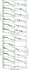 |
Fig. B.1. Comparison between models and observations. The open circles show the observed bolometric LCs (left) and Fe II velocities (right). Solid lines represent 30 models randomly chosen from the probability distribution. The panels present SNe in order of their discovery dates, from SN 2004ej to SN 2005dt. Grey shaded regions show the early data we removed from the fitting. The errors in the observed bolometric LCs are not plotted, for better visualisation. |
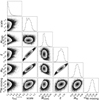 |
Fig. B.5. Corner plot of the joint posterior probability distribution of the parameters for SN 2006ai. |
SN II physical parameters.
Appendix C: High-mass progenitor fits
We mapped LCs and expansion velocities from high-mass models as observations to test our fitting technique. Figure C.1 shows a corner plot of the joint posterior probability distribution of the parameters for a model of MZAMS = 24 M⊙, E = 1.4 foe, MNi = 0.03 M⊙, and 56Ni mixing = 0.5. The blue squares represent the input physical parameters of the model.
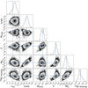 |
Fig. C.1. Corner plot of the joint posterior probability distribution of the parameters when a high-mass progenitor model is considered as observations for our fitting technique. Blue squares represent the input physical parameters of the model. |
Appendix D: High-mass progenitor models evolved with enhanced mass loss
In Sect. 7.2 we proposed that one possible solution for the IMF incompatibility could be to consider a higher rate of mass loss, in addition to a larger mixing-length parameter. A detailed investigation is beyond the scope of this work; however, we give an example to show that our suggestion allows high-MZAMS progenitors to fit some SNe II in the CSP-I sample.
We used MESA (Paxton et al. 2011, 2013, 2015, 2018, 2019) to obtain pre-SN models employing the same configurations detailed in Sect. 4, with two exceptions. We adopted a wind scaling factor of η = 1.5 (i.e. 50% higher than standard) and a mixing-length parameter of three. Then, we used the code presented in Bersten et al. (2011) to obtain bolometric LC and photospheric velocity models. We generated a small grid of models for MZAMS = 20 and 22 M⊙, E = 0.8, 1.0, and 1.2 foe, MNi = 0.03 M⊙, and 56Ni mixing = 0.8 (given in fraction of the pre-SN mass). Thus, we obtained a total of six hydrodynamical models.
We used these six models to compare with all CSP-I SNe II with bolometric luminosities during the photospheric phase and – at least – the transition to the radioactive tail and velocity measurements. The observations of a small number of SNe II in the CSP-I sample can be reasonably reproduced by some of these models. We discuss the case of SN 2006ai as an example. The 20 M⊙ models reproduce the plateau phase and the transition to the radioactive phase. The models display lower luminosities during the radioactive tail phase, indicative of a higher 56Ni mass in the ejecta of SN 2006ai than that assumed in the models. For this reason, we carried out new models with higher 56Ni masses until the observed radioactive tail phase is reproduced by our models. Figure D.1 shows the models that reproduce the observations of SN 2006ai12. Both models assume MZAMS = 20 M⊙, MNi = 0.049 M⊙, and 56Ni mixing = 0.8. Model 1 and Model 2 were exploded with E = 1.0 and 1.2 foe, respectively. We stress that this test seeks reasonable agreement between models and observations and not detailed fits to observations. A fine tuning of the model parameters is required to find the best-fitted model.
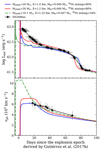 |
Fig. D.1. Observed bolometric LC (top panel) and Fe IIλ5169 line velocities of SN 2006ai (black markers). Solid lines represent the high-MZAMS models with increased mass loss that best reproduce the observations. Dashed lines represent the maximum a posteriori model using our standard grid of models. This model is corrected by the scale factor and the explosion epoch found in Sect. 5. Since our estimation suggests an earlier explosion epoch, the model shown as dashed lines starts before zero on the x axis (where zero corresponds to the explosion epoch derived by Gutiérrez et al. 2017b). |
This test shows that a high-MZAMS progenitor evolved with enhanced mass loss and larger mixing-length parameter can reproduce the observations of a SN II (i.e. in the direction to solve the IMF incompatibility). However, a deeper analysis is necessary for stronger conclusions.
All Tables
All Figures
|
Fig. 1. Observed bolometric LC (top panel) and Fe IIλ5169 line velocities (bottom panel) of SN 2006ai (filled markers) with models randomly sampled from the posterior distribution of the parameters (solid lines). The median value and 68% confidence range for every physical parameter are also shown. The grey shaded region shows the early data removed from the fitting (first 30 days after explosion). |
| In the text | |
|
Fig. 2. Histograms of three progenitor parameters: MZAMS (top panel), Mej (middle panel), and R (bottom panel). The gold sample is represented by yellow bars, and the red bars are the histograms for the full sample. In each panel, the number of SNe II is listed, together with the median and the 16th and 84th percentiles. Probability density functions of the physical parameters for the gold and full samples are represented by solid and dashed lines, respectively. |
| In the text | |
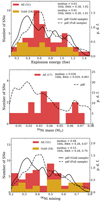 |
Fig. 3. Same as in Fig. 2 but for E (top panel), MNi (middle panel), and 56Ni mixing (bottom panel). |
| In the text | |
|
Fig. 4. Cumulative distribution of MZAMS for the SN II progenitors in the gold sample. The derived masses are shown in yellow squares. The shaded contours show the confidence regions of the CD. |
| In the text | |
|
Fig. 5. Same as in Fig. 4 but for the SN II progenitors in the full sample. Yellow squares represent the SNe II in the gold sample. |
| In the text | |
|
Fig. 6. Fits to the CD of MZAMS of SN II progenitors in the gold sample. Left panel: CD of MZAMS derived in our work for the gold sample (yellow triangles and error bars), corresponding to the median and the 68% confidence limit of the distribution presented in Fig. 4 as shaded contours, in comparison with the model CD constructed with the median values of the marginal distributions of the parameters (shaded contours). Right panel: corner plot of the joint posterior probability distribution of the parameters. Dashed lines indicate the 16th, 50th, and 84th percentiles of the distributions. |
| In the text | |
|
Fig. 7. Same as in Fig. 6 but when the power-law slope is fixed to Γ = −2.35, that is, the slope of a Salpeter massive-star IMF. |
| In the text | |
|
Fig. 8. Fits to the CD of MZAMS of SN II progenitors in the full sample. Top left: CD of MZAMS derived in our work for the full sample (red triangles and the error bars), corresponding to the median and the 68% confidence limit of the distribution presented in Fig. 5 as shaded contours, in comparison with the model CD constructed with the median values of the marginal distributions of the parameters (shaded contours). Bottom left: corner plot of the joint posterior probability distribution of the parameters. Dashed lines indicate the 16th, 50th, and 84th percentiles of the distributions. The right panels show the same as the left panels but when the power-law slope is fixed to Γ = −2.35. |
| In the text | |
|
Fig. 9. Comparison of ejecta masses (top panel) and explosion energies (bottom panel) derived in the current work to those from previous studies containing large samples of SNe II. |
| In the text | |
|
Fig. 10. Best-fitting power-law slope of the CD of the progenitor masses for a range of sample sizes. The error bars correspond to the 68% confidence limit. The larger the sample, the higher the probability that the best-fitting power-law slope is that of a Salpeter IMF. The solid black line indicates the Salpeter IMF slope for massive stars. |
| In the text | |
|
Fig. B.1. Comparison between models and observations. The open circles show the observed bolometric LCs (left) and Fe II velocities (right). Solid lines represent 30 models randomly chosen from the probability distribution. The panels present SNe in order of their discovery dates, from SN 2004ej to SN 2005dt. Grey shaded regions show the early data we removed from the fitting. The errors in the observed bolometric LCs are not plotted, for better visualisation. |
| In the text | |
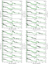 |
Fig. B.2. Same as in Fig. B.1, but from SN 2005dw to SN 2008K. |
| In the text | |
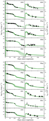 |
Fig. B.3. Same as in Fig. B.1, but from SN 2008M to SN 2009N. |
| In the text | |
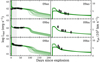 |
Fig. B.4. Same as in Fig. B.1, but from SN 2009ao to SN 2009bz. |
| In the text | |
|
Fig. B.5. Corner plot of the joint posterior probability distribution of the parameters for SN 2006ai. |
| In the text | |
|
Fig. C.1. Corner plot of the joint posterior probability distribution of the parameters when a high-mass progenitor model is considered as observations for our fitting technique. Blue squares represent the input physical parameters of the model. |
| In the text | |
|
Fig. D.1. Observed bolometric LC (top panel) and Fe IIλ5169 line velocities of SN 2006ai (black markers). Solid lines represent the high-MZAMS models with increased mass loss that best reproduce the observations. Dashed lines represent the maximum a posteriori model using our standard grid of models. This model is corrected by the scale factor and the explosion epoch found in Sect. 5. Since our estimation suggests an earlier explosion epoch, the model shown as dashed lines starts before zero on the x axis (where zero corresponds to the explosion epoch derived by Gutiérrez et al. 2017b). |
| In the text | |
Current usage metrics show cumulative count of Article Views (full-text article views including HTML views, PDF and ePub downloads, according to the available data) and Abstracts Views on Vision4Press platform.
Data correspond to usage on the plateform after 2015. The current usage metrics is available 48-96 hours after online publication and is updated daily on week days.
Initial download of the metrics may take a while.