| Issue |
A&A
Volume 660, April 2022
|
|
|---|---|---|
| Article Number | A46 | |
| Number of page(s) | 17 | |
| Section | Stellar atmospheres | |
| DOI | https://doi.org/10.1051/0004-6361/202141970 | |
| Published online | 12 April 2022 | |
Abundance of zirconium in the globular cluster 47 Tucanae: a possible Zr–Na correlation?*,**
1
Institute of Theoretical Physics and Astronomy, Vilnius University,
Saulėtekio al. 3,
Vilnius,
10257,
Lithuania
e-mail: This email address is being protected from spambots. You need JavaScript enabled to view it.
2
GEPI, Observatoire de Paris, Université PSL,
CNRS, 5 place Jules Janssen,
92190
Meudon,
France
3
Crimean Astrophysical Observatory,
Nauchny
298409,
Crimea
Received:
5
August
2021
Accepted:
9
November
2021
Abstract
We determined abundances of Na and Zr in the atmospheres of 237 RGB stars in Galactic globular cluster (GGC) 47 Tuc (NGC 104), with a primary objective of investigating possible differences between the abundances of Zr in the first generation (1P) and second generation (2P) stars. For the abundance analysis, we used archival UVES/GIRAFFE spectra obtained during three different observing programmes. Abundances were determined from two Na I and three Zr I lines, using 1D hydrostatic ATLAS9 model atmospheres. The target stars for the abundance analysis were limited to those with 4200 ≤ Teff ≤ 4800 K. This is the largest sample of GGC stars in which Na and Zr abundances have been studied so far. While our mean [Na/Fe] and [Zr/Fe] ratios agree well with those determined in the earlier studies, we find a weak but statistically significant correlation in the [Zr/Fe] – [Na/Fe] plane. A comparison of the mean [Zr/Fe] abundance ratios in the 1P and 2P stars suggests a small but statistically significant Zr over-abundance in the 2P stars, ∆[Zr/Fe]2P−1P ≈ +0.06 dex. Also, our analysis shows that stars enriched in both Zr and Na are more centrally concentrated. However, we find no correlation between their distance from the cluster centre and their full spatial velocity, as indicated by the velocity dispersions at different mean values of [Zr/Fe] and [Na/Fe]. While there may be some influence of CN line blends on the determined Zr abundances, it seems very unlikely that the detected Zr–Na correlation, for the slightly higher Zr abundances in the 2P stars, would be caused by the CN blending alone. The obtained results indicate that, in 47 Tuc, some amount of Zr should have been synthesised by the same polluters that enriched 2P stars with the light elements. While sizeable amounts of Zr may be synthesised by both AGB stars (M ~ 1.5–5 M⊙) and massive rotating stars (M ~ 12–25 M⊙, υrot > 150 km s−1), our data alone do not allow us to distinguish which of the two scenarios, or whether or not a combination of both, could have operated in this GGC.
Key words: techniques: spectroscopic / stars: abundances / stars: late-type / globular clusters: individual: 47 Tuc
Table D.1 is only available at the CDS via anonymous ftp to cdsarc.u-strasbg.fr (130.79.128.5) or via http://cdsarc.u-strasbg.fr/viz-bin/cat/J/A+A/660/A46
Based on observations obtained at the European Southern Observatory (ESO) Very Large Telescope (VLT) at Paranal Observatory, Chile.
© ESO 2022
1 Introduction
Nearly all Galactic globular clusters (GGCs) studied until now exhibit spreads and correlations (or anti-correlations) between the abundances of light chemical elements; for example the O–Na, Mg–Al (Carretta et al. 2009), and Li–O (Pasquini et al. 2005; Shen et al. 2010) anti-correlations, and the Na–Li (Bonifacio et al. 2007) correlation. Evolutionary scenarios proposed to explain these trends typically assume that stars in the GGCs formed during several star formation episodes and that the second-generation (2P) stars were polluted with light chemical elements synthesised in the first-generation (1P) stars. Various candidate polluters have been proposed, including fast-rotating massive stars (FRMS; e.g. Decressin et al. 2007), asymptotic giant branch (AGB) stars (e.g. D’Antona et al. 2016), and super-massive stars (~104 M⊙, SMS; e.g. Denisenkov & Hartwick 2014;Gieles etal. 2018).
In contrast to the light elements, variations in the abundances of neutron-capture elements (s-process and r-process elements) are less commonly reported and have been observed only in a few GGCs which belong to a class of so-called anomalous or Type-II clusters (Marino et al. 2015, Marino et al. 2019). Type-II clusters are amongst the most massive ones (> 106 M⊙) and are characterised by significant spreads in the abundance of Fe and Fe-group elements (e.g. Marino et al. 2019). Although the remaining GGCs, namely Type-I, are generally homogeneous in the s-process abundances, there have been claims that relations between the abundances of s-process and light elements may exist in some Type I GGCs as well (see e.g. Gratton et al. 2013; Yong et al. 2013). For example, Gratton et al. (2013) suggested the existence of a Na-Ba correlation in the red horizontal branch (RHB) stars of one of the closest GGCs, 47 Tuc. However, this finding was not corroborated by further investigation of this cluster (e.g. Cordero et al. 2014; Thygesen et al. 2014). Unfortunately, studies of the s-process elements in 47 Tuc (and in the majority of the other GGCs) have mostly been based on relatively small stellar samples. This makes it difficult to make a robust statistical assessment of the abundance spreads and correlations.
To partly fill this gap, we determined abundances of Na and Zr in 237 red giant branch (RGB) stars in 47 Tuc. This is the largest stellar sample used to study s-process elements in any GGC so far. As discussed in Prantzos et al. (2018), evolution of Zr in the Galaxy is well reproduced by nucleosynthesis in massive rotating stars. Theoretical models predict that light s-process elements (Sr, Y, Zr) are produced in AGB stars (1.5–5 M⊙) or massive stars (>9 M⊙) during weak s-process nucleosynthesis, while the heavier s-process elements (Ba, La, etc.) are synthe-sised mostly in lower-mass AGB stars, via the main s-process (e.g. Cristallo 2018). Thus, the detection of correlations between the abundances of light and s-process elements may allow more stringent constraints to be placed on the nature of possible polluters.
Spectroscopic data used in this work.
2 Observational data and atmospheric parameters
2.1 Spectroscopic data and determination of atmospheric parameters
Abundances of Fe, Na, and Zr were determined using VLT/GIRAFFE spectra that were obtained during three observing programmes (Table 1) and downloaded for the analysis from the ESO Advanced Data Products archive1. The data were taken during three observing programmes: 072.D-0777(A) (PI: P. François); 073.D-0211(A) (PI: E. Carretta); 088.D-0026(A) (PI: I. McDonald). The median sky spectrum was subtracted from each individual stellar spectrum, and the remaining spectra were then continuum normalised using the IRAF splot task (Tody 1986). Each object in the programme 088.D-0026(A) was observed multiple times, therefore the sky-subtracted spectra from the individual exposures were co-added together. The typical signal-to-noise ratios in the spectra were S/N ~ 70–150 at 620 nm.
The effective temperatures of the target RGB stars were determined using photometric observations from Bergbusch & Stetson (2009) and the Teff − (V − I) calibration of Ramírez & Meléndez (2005). Although Gaia EDR3 photometry for the target stars was also available, we decided to use photometric data from Bergbusch & Stetson (2009) in order to retain homogeneity and consistency with our previous studies of 47 Tuc (see e.g. Dobrovolskas et al. 2014; Černiauskas et al. 2017). The average difference between the effective temperatures determined using (V − I) colour indices and those obtained from the Gaia EDR3 photometry and colour-effective temperature calibration from Mucciarelli et al. (2021) is ~−59 K and does not affect the results obtained in this study. To check the reliability of our Teff estimates, we determined Fe abundances in 111 RGB stars in the 073.D-0211(A) sample using a set of Fe I lines (see Appendix B.2.1) and effective temperatures from photometry. On average, the residual slopes of the iron abundance versus the line excitation potential were smaller than 0.03 dex eV−1 with a typical 1σ slope uncertainty of 0.04 dex eV−1, suggesting good agreement between the photometric and spectroscopic effective temperatures.
Surface gravities of the target stars were determined using the classical relation between stellar mass, luminosity, effective temperature, and surface gravity. We assumed an identical mass of 0.89 M⊙ for all target RGB stars, as determined from the Yonsei-Yale isochrone2 (12 Gyr, [M/H] = −0.68; Kim et al. 2002). We did not use spectroscopic gravities: although there were four Fe II lines available in the wavelength range of GIRAFFE spectra, accurate equivalent width (W) measurements were possible for only two or three lines per target star spectrum which was insufficient for reliable gravity determination. Nevertheless, the mean iron abundance obtained for the entire sample of stars using Fe I and Fe II lines agrees to within 0.01 dex. For any particular star, the largest difference between the two Fe abundance estimates never exceeded 0.1 dex. This suggests good agreement between the surface gravities determined from photometry and those obtained via the ionisation balance condition.
After visual inspection of the target star positions in the Teff − log g diagram, we discarded 36 horizontal branch (HB) and AGB stars in the sample of 072.D-0777(A). We also discarded four HB stars from the 088.D-0026(A) sample and one HB star from the sample of 073.D-0211(A). The determined effective temperatures and gravities of the target stars are shown in Fig. 1 and are listed in Table D.1.
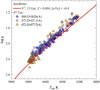 |
Fig. 1 Atmospheric parameters of the target RGB stars. Stars observed in different programmes are shown in different symbols and colours: orange triangles – 072.D-0777(A), grey circles – 073.D-0211(A), blue diamonds – 088.D-0026(A). The Yonsei-Yale isochrone of 12 Gyr and [M/H] = -0.68, and [a/Fe] = +0.4 is shown for comparison as a red solid line (Kim et al. 2002). |
2.2 Radial velocities, proper motions, and cluster membership
Radial velocities of the target stars were measured from the VLT/GIRAFFE spectra using the cross-correlation method with the IRAF task fxcor. For cross-correlation, we used the ATLAS9 model with Teff = 4500 K, log g = 1.90, [Fe/H] = −0.7 to compute a synthetic spectrum with R = 22000 in the wavelength range of 612–640 nm using SYNTHE. We obtained a mean value for radial velocity of −17.4 km s−1 (σ = 7.9 km s−1) with a typical measurement error of ±0.1 km s−1 for individual stars. Stars with radial velocities falling within ±3σ of the mean cluster radial velocity were assigned as cluster members.
Full spatial velocities of our target stars were obtained by combining their radial velocities (determined by us) with their proper motions from the Gaia EDR3 catalogue (Gaia Collaboration 2021). We matched the coordinates of the target stars (taken from Bergbusch & Stetson 2009) with those of stars in the Gaia EDR3 catalogue using a 1″ matching radius. The average proper motion of 47 Tuc, µRA = 5.25 mas yr−1 and µDec = −2.53 mas yr−1, was taken from Baumgardt et al. (2019) and the proper motions of individual stars were computed relative to the average proper motion of the cluster. Following Milone et al. (2018), targets were selected as cluster members if their proper motions did not deviate by more than 1.5 mas yr−1 from the mean cluster proper motion. Based on this consideration, 13 stars were rejected from further analysis (Fig. 2).
Finally, we converted the proper motions from angular units to tangential velocities in km s−1 assuming the distance of 4.5 kpc to 47 Tuc. The obtained radial and tangential velocities were used to compute full spatial velocities. After rejecting the likely non-members based on kinematical considerations, we further restricted our target sample to stars with 4200 ≤ Teff ≤ 4800 K. This was done in order to limit the influence of uncertainties on the abundances determined at the lower and higher ends of Teff range (see Sect. 3).
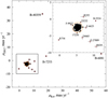 |
Fig. 2 Proper motions of the target RGB stars from the Gaia EDR3 catalogue (Gaia Collaboration 2021). Identifications of non-member stars are shown next to the symbols. The region that encloses motions falling within 1.5 mas yr-1 from the mean cluster proper motion is marked by a orange circle. Stars falling outside this region were rejected from the abundance analysis. Zoomed-in region marked by a square is shown in the top right corner. |
3 Determination of abundances
Elemental abundances were determined using the 1D hydrostatic ATLAS9 model atmospheres (Kurucz 1993; Sbordone et al. 2005) enhanced in the α-element abundances (O, Ne, Mg, Si, S, Ar, Ca, Ti) by [α/Fe] = +0.4. In cases where target star spectra were available from several observing programmes, abundances of Fe, Na, and Zr were determined from each individual spectrum and average abundances were used for further analysis. The equivalent width method was used for obtaining abundances of Fe and Zr (but also see Sect. 3.3 below) while the Na abundances were measured by performing spectral line synthesis.
The stars used in the abundance analysis were limited to those with effective temperatures in the range 4200 ≤ Teff ≤ 4800 K. This choice was made because: (a) uncertainties in the continuum determination and a possible influence of molecular blends become higher at lower temperatures and lead to larger errors in Zr abundances; (b) uncertainties in the Zr abundances increase significantly due to weaker Zr I lines at higher temperatures; and (c) at higher Teff, Zr I lines become increasingly too weak to be detected in stars with the lowest Zr abundance. The final sample thus consists of 237 RGB stars (Appendix A).
Examples of the Na I and Zr I line fits are shown in Fig. 3 where we also provide a synthetic spectrum computed with Zr abundance set to zero to indicate a possible influence of CN lines on the determined Zr abundances (this effect is discussed in Sect. 4.3). Abundances of Fe, Na, and Zr determined in the individual stars are provided in Table D.1. Details of the abundance determination process are provided in Sects. 3.1–3.3 below.
3.1 Abundance of Fe
Local thermodynamic equilibrium (LTE) was assumed in the analysis of Fe abundances which were determined using the equivalent width method. Abundances were obtained using a set of 17–28 Fe I lines (612.79–691.67 nm), where the lower level excitation potentials of the lines are in the range of 2.18–4.61 eV (Table B.1).
Microturbulence velocities, ξmicro, were determined alongside Fe abundances by enforcing a zero trend of Fe I abundances with the line equivalent width. We discarded strong lines (W > 15 pm) because of their lower sensitivity to ξmicro. The obtained ξmitro are plotted versus Teff in Fig. 4. The typical accuracy of the determined ξmicro values was ±0.2 km s−1 and was constrained by the number of Fe I lines (17–28) available.
Iron abundances determined in the individual RGB stars are provided in Table D.1. The obtained abundances show no strong dependence on either ξmicro or Teff. In addition, no significant discrepancies are seen in abundances determined using data from different observing programmes (Appendix B.2.1).
3.2 Abundance of Na
In the case of Na, abundances were measured assuming nonlocal thermodynamic equilibrium (NLTE) in the spectral line synthesis computations that were performed using the MULTI code (Carlsson 1986; Korotin et al. 1999). The Na model atom used in the analysis consisted of 20 levels of Na I and the ground state of Na II, with 46 radiative transitions between the different atomic levels. Collision rates with electrons and hydrogen were taken from Igenbergs et al. (2008) and Barklem et al. (2010) respectively (see Dobrovolskas et al. 2014, for details). Two Na I lines located at 615.4225 and 616.0747 nm were used in the analysis. Synthetic line profiles were computed with the MULTI code and were broadened with a Voigt profile to account for the instrumental and macroturbulence broadening. We used microturbulence velocities that were determined individually for each target star. The abundance of Na and macroturbulence velocity were then determined iteratively to achieve the best fit of the synthetic line profiles to the observed spectra (Fig. 3).
No significant systematic differences are seen in Na abundances obtained from the two Na I lines or those determined using data from different observing programmes. There is a hint of a weak dependence of Na abundance on Teff but it does not exceed 0.1 dex (see Appendix B.2.2). The Na abundances determined in the target RGB stars are provided in Table D.1.
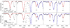 |
Fig. 3 Observed (dots) and best-fitted synthetic profiles of the Na I (NLTE) and Zr I (LTE) lines (red solid lines) in the GIRAFFE spectra of two RGB stars in 47 Tuc: Na-rich (23175, 2P, top row) and Na-poor (R266, 1P, bottom row). Identification numbers of each star, their atmospheric parameters, and the determined Na and Zr abundances are provided in the leftmost panels of each row. The blue lines show synthetic spectrum computed with A(Zr) = 0 to show the possible influence of CN and other blends (further discussed in Sect. 4.3.). |
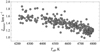 |
Fig. 4 Microturbulence velocity in the target RGB stars, ?micro, versus the effective temperature of individual stars. |
3.3 Abundance of Zr
3.3.1 Zr abundance from Zr I lines
Abundances of Zr were determined with the WIDTH9 code (Sbordone et al. 2005; Kurucz 2005a) using three Zr I lines located at 612.7475, 613.4585, and 614.3252 nm (Table B.2). Line equivalent widths were measured by fitting Gaussian profiles with the splot task in IRAF. Because the 612.7475 nm Zr I line is blended with the Fe I 612.7906 nm line, the equivalent width of the former was determined using the IRAF task deblend. In addition, all Zr I lines used in our study were affected by weak CN blends. We did not take this effect into account when measuring line equivalent widths but we did investigate its possible influence on the determined Zr abundances and did not find it to be critical (see Sect. 4.3 for details). The final Zr abundances were obtained by averaging the measurements of all three Zr I lines.
For the abundance determination, we used an updated Zr I ionisation energy of 6.634 eV from Hackett et al. (1986) instead of the default value of 6.840 eV implemented in the original versions of the Kurucz ATLAS9, WIDTH9, and SYNTHE packages (Sbordone et al. 2005). This led to a systematic change in zirconium abundance of +0.29 dex at Teff = 4200 K and +0.25 dex at Teff = 4800 K.
There is good agreement between Zr abundances obtained from the three Zr I lines and those determined using data from different observing programmes. The obtained abundances do not show trends with the microturbulence velocity or Teff (see Appendix B.2.3). Abundances of Zr obtained for the individual target RGB stars are provided in Table D.1.
It is important to stress that in our analysis, the hyperfine structure splitting (HFS) of Zr I lines was not taken into account. To assess its influence, we synthesised all three Zr I lines with and without taking HFS into account. For this, we used the ATLAS9 model atmosphere with Teff = 4320 K, log g = 1.52, ξmicro = 1.56 km s−1, [Fe/H] = −0.78, and [α/Fe] = +0.4. The effective temperature of the model atmosphere is similar to those of the ‘coolest’ stars in our sample (Teff ≈ 4200 K). Because at a given Zr abundance Zr I lines are stronger in stars with lower Teff, one may anticipate larger HFS-related effects at the lower end of the Teff scale. Spectral line synthesis was done with the SYNTHE package. Line oscillator strengths for the individual HFS components were taken from Thygesen et al. (2014) while for the computation of line profiles without HFS these components were added up for each Zr I line (Table 2). We used A(Zr) = 2.16 for both HFS and non-HFS lines. The equivalent widths of synthetic lines were measured by fitting the Gaussian profile, and abundances of Zr were determined from the obtained equivalent widths using the WIDTH9 code. As seen from Table 2, the largest abundance difference of +0.02 dex is seen in the case of the 612.7475 nm line, while the difference for lines at 613.4585 and 614.3252 nm is smaller than 0.01 dex. At higher Teff values, the differences are even smaller because the Zr I lines are weaker. We therefore conclude that HFS of the Zr I lines does not have a significant impact on Zr abundances determined in our study.
The 088.D-0026(A) sample contains one star – ‘R265’ or ‘Lee 4710’ – which is strongly enriched in s-process elements (Cordero et al. 2015). For this star, we determined a zirconium abundance of [Zr/Fe] = 0.79 ± 0.15 (error is standard deviation due to line-to-line abundance scatter), which is in very good agreement with the value of 0.83 ± 0.17 obtained by Cordero et al. (2015). The atmospheric parameters of the star determined in both studies also agree very well: we obtained Teff = 4452 K, log g = 1.82, ξmicro = 1.55 km s−1, and [Fe/H] = −0.79 while Cordero et al. (2015) derived Teff = 4475 K, log g = 1.60, ξmicro = 1.65 km s−1, and [Fe/H] = −0.78. Due to its anomalous abundance patterns, Lee 4710 was excluded from further analysis.
Impact of HFS on the determination of Zr abundance from the Zr I lines used in this study.
3.3.2 Zr abundance from Zr II lines
To some extent, the robustness and reliability of Zr abundances obtained from Zr I lines may be assessed by comparing them with those determined using Zr II lines. Unfortunately, no existing VLT/GIRAFFE observations of 47 Tuc extend over the wavelengths of Zr II lines. We therefore used VLT/UVES spectra of 13 RGB stars in 47 Tuc obtained by Thygesen et al. (2014) whose wavelength range covers several Zr II lines. Although the authors focused on the coolest RGB stars in 47 Tuc, there are three stars with 4200 ≤ Teff ≤ 4800 K (our Teff scale) that have been observed both in their UVES and our GIRAFFE samples. To the best of our knowledge, these are the only archival UVES spectra of our GIRAFFE targets which cover the wavelength range of Zr II lines.
The results of our analysis of the three stars suggest good agreement between Zr abundances obtained using Zr I and Zr II lines (see Appendix B.2.4 for details). Even in the extreme cases, the differences do not exceed 0.10 dex. For each star, the corresponding averages obtained from Zr I and Zr II lines show even better agreement, with the differences being smaller than 0.03 dex. We therefore conclude that, despite the small number of stars used in this test, the consistency of Zr abundances obtained from individual Zr I and Zr II lines nevertheless suggests that the influence of various effects (NLTE, line blends, line data, systematic errors in the analysis procedures, etc.) on the determined Zr abundances is likely minor (the case of CN blends is discussed separately in Sect. 4.3).
3.4 Abundance determination errors
To estimate the errors in the determined abundances of Fe, Na, and Zr, we followed the prescription provided in Černiauskas et al. (2017). Briefly, we account for the uncertainties in stellar parameters, continuum determination, and line profile fitting, with the final abundance errors determined by adding error components in quadrature. Detailed descriptions of the methodology, error determination procedure, and the determined abundance errors are provided in Appendix B.2.5, with typical values being in the range of 0.09–0.16 dex (Tables B.5–B.7).
Minimum, maximum, and mean Fe, Na, and Zr abundance ratios determined in the sample of 237 RGB stars in 47 Tuc.
4 Results and discussion
4.1 Mean abundances of Fe, Na, and Zr in the target RGB stars in 47 Tuc
For the sample of 237 stars (4200 ≤ Teff ≤ 4800 K, Sect. 3), we obtained a mean 〈[Fe/H]〉 = −0.75 ± 0.05 (Table 3; the error denotes standard deviation due to the star-to-star abundance scatter). This agrees well with the values determined in earlier studies (e.g. 〈[Fe/H]〉 = −0.74 ± 0.05 by Carretta et al. 2009, for 114 RGB stars; 〈[Fe/H]〉 = −0.77 ± 0.08 by Wang et al. 2017, for 44 RGB stars), as well as with the mean iron abundance measured by us for the same target stars using Fe II lines (〈[Fe/H]Fe II〉 = −0.73 ± 0.093). For reference, we used the solar iron abundance of A(Fe)⊙ = 7.55 ± 0.06 that was determined in Appendix B.1 utilizing the same set of Fe I lines as in the analysis of target RGB stars in 47 Tuc.
As expected, the obtained [Na/Fe] ratios show a considerable range of scatter, 0.05 ≤ [Na/Fe] ≤ 0.78, with a mean value of 〈[Na/Fe]〉 = 0.41 ± 0.16 (Table 3; we remind that abundances of Na were determined assuming NLTE and those of Fe using LTE). The scatter range, as well as the mean [Na/Fe] value, agree well with those obtained in other studies; for example ∆[Na/Fe] = 0.76 and 〈[Na/Fe]〉 = 0.47 ± 0.15 (Carretta et al. 2009, 147 RGB stars), ∆[Na/Fe] = 0.56 and 〈[Na/Fe]〉 = 0.36 ± 0.18 (Wang et al. 2017, 27 RGB stars).
For Zr, the range of star-to-star scatter is similar to that obtained for Na, 0.11 ≤ [Zr/Fe] ≤ 0.68, with a mean value of 〈[Zr/Fe]〉 = 0.35 ± 0.09 (Table 3). Again, the mean value and abundance dispersion due star-to-star scatter agree well with those obtained in earlier studies; for example 〈[Zr/Fe]〉 = 0.52 ± 0.03 (Worley et al. 2010, 5 AGB stars), and 〈[Zr/Fe]〉 = 0.41 ± 0.19 (Thygesen et al. 2014, 13 RGB stars). A larger difference is seen when comparing with the results of Wylie et al. (2006, average in seven rGb/AGB stars) who obtain 〈[Zr/Fe]〉 = 0.69 ± 0.15.
4.2 A possible Zr–Na correlation?
The obtained Zr and Na abundances suggest the existence of a weak correlation in the [Zr/Fe] – [Na/Fe] plane (Fig. 5, top). To estimate its statistical significance, we assumed a null hypothesis that the Pearson’s and the non-parametric Spearman’s and Kendall’s correlation coefficients (r, ρ, and τ, respectively) are zero in this plane, that is, that the two abundance ratios are uncor-related. Although the determined correlation coefficients suggest of 47 Tuc (rh = 174″, Trager et al. 1993). This is in line with the findings of previous studies of this and other GGCs (see e.g. Bastian & Lardo 2018). The p-values computed for all correlation coefficients are extremely small (Table 4).
A qualitatively similar picture is seen also in the [Zr/Fe]. [Na/Fe] plots constructed using stars divided into bins of μTeff = 100 K. Here, we obtained p < 0.05 in all but one of the temperature bins, namely 4400 < Teff < 4500 K; Fig. 6.
Our data also indicate that stars with the highest [Na/Fe] and [Zr/Fe] ratios tend to concentrate towards the cluster centre, as suggested by trends seen in the [Zr/Fe]-r/rh and [Na/Fe]-r/rh planes (Fig. 5), where r is the projected distance from the cluster centre of the given target star and rh is the half-light radius of 47 Tuc (rh = 174′, Trager et al. 1993). This is in line with the findings of previous studies of this and other GGCs (see e.g. Bastian & Lardo 2018). The p-values computed for all correlation coefficients are extremely small (Table 4).
We find no correlation between the [Zr/Fe] and [Na/Fe] ratios and the full spatial velocities of the target stars (Fig. 7). Similarly, there is no statistically significant correlation between the two abundance ratios and velocity dispersions computed in the non-overlapping 0.1 dex-wide abundance bins, as indicated by the results of the t-test and the Levene’s test (Fig. 8; see also Appendix C; we note that this result is not affected by the size of the binning step and/or whether the bins are overlapping or not). This is in contrast to the findings of Kučinskas et al. (2014) who, based on the analysis of 101 TO stars in 47 Tuc, detected a weak but statistically significant correlation between the radial velocity dispersion and [Na/O] and [Li/Na] abundance ratios. One possible explanation for this discrepancy is that [Na/O] shows a significantly larger 1P–2P variation range (>1 dex) than the [Na/Fe] or [Zr/Fe] ratios which may make the detection of a possible correlation more difficult in the latter two cases. Nevertheless, while our stellar sample is more than two times larger, we find no differences in the kinematical properties of 1P and 2P stars as traced by the [Na/Fe] and/or [Zr/Fe] abundance ratios.
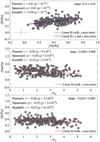 |
Fig. 5 [Zr/Fe] ratios in the sample of 237 RGB stars in 47 Tuc. Top panel: [Zr/Fe] versus [Na/Fe] ratios. Middle and bottom panels, respectively: [Zr/Fe] and [Na/Fe] ratios versus projected distance from the cluster centre, r/rh. Linear least-square best fits are shown as solid lines, fit parameters, correlation coefficients, and the p-values are provided in each individual panel. Typical errors of the individual abundance measurements are indicated in the top panel. |
Pearson, Spearman and Kendall correlation coefficients and the corresponding p-values in the [Zr/Fe]–[Na/Fe] and abundance–distance planes.
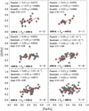 |
Fig. 6 [Zr/Fe] – [Na/Fe] plots for stars divided into bins of ?Teff = 100 K (N is the number of stars in each bin). Values of different correlation coefficients and the corresponding p-values are provided for each temperature bin. |
4.3 Influence of CN blends on the determined Zr abundances
One issue of concern is that all three Zr I lines used in this study are blended with CN lines (see Figs. 3, 9). Because abundances of C and N differ significantly in the 1P and 2P stars (e.g. Carretta et al. 2005; Mészáros et al. 2020), the strengths of CN blends will differ as well. This may lead to systematically stronger blended lines (i.e. Zr+CN) and higher Zr abundances in the 2P stars when measured from the line equivalent widths without taking the influence of CN lines into account (i.e. as was done in our study because abundances of C and N are not known for all target stars; see Sect. 4.3.2). Because the 2P stars have higher Na abundances, the CN blends may therefore lead to systematically overestimated Zr abundances in these stars, which in turn may produce a spurious correlation between Zr and Na abundances. We carried out two tests to assess the possible influence of CN blends, the results of which are described below.
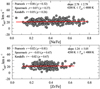 |
Fig. 7 Full spatial velocities of 237 RGB stars in 47 Tuc versus their [Na/Fe] and [Zr/Fe] ratios (top and bottom, respectively). |
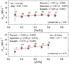 |
Fig. 8 Dispersions of full spatial velocities of the target RGB stars computed in non-overlapping [Zr/Fe] (top panel) and [Na/Fe] (bottom panel) abundance bins of 0.1 dex. Solid lines are linear least-square fits and the number of stars in each abundance bin is indicated next to each data point. Indicated are the p-values that were obtained using different methods (including the Levene’s test, see Appendix C), and error bars were computed using the bootstrapping technique. |
4.3.1 Influence of CN blends estimated using extreme C and N abundances
For the first test, we computed synthetic profiles of the three Zr I lines at 612.7475, 613.4585, and 614.3252 nm, with the CN line profiles calculated using CNO abundances determined in the 1P and 2P stars of this GGC from the APOGEE-2 data by Mészáros et al. (2020, 82 RGB stars in total). For this, we selected three sets of CNO abundances corresponding to the CN-weak, CN-intermediate, and CN-strong lines:
![Mathematical equation: $\matrix{ - \hfill & {\left[ {{\rm{C/Fe}}} \right] = + 0.20,\,\left[ {{\rm{N/Fe}}} \right] = + 0.20,\,\left[ {{\rm{O/Fe}}} \right] = + 0.80\,\left( {{\rm{case - A}},} \right.} \hfill \cr {} \hfill & {\left. {\quote {\rm{CN - weak}}\quote ,\,{\rm{1P}};} \right)} \hfill \cr - \hfill & {\left[ {{\rm{C/Fe}}} \right] = - 0.20,\,\left[ {{\rm{N/Fe}}} \right] = + 1.10,\,\left[ {{\rm{O/Fe}}} \right] = + 0.60\,\left( {{\rm{case - B}},} \right.} \hfill \cr {} \hfill & {\left. {\quote {\rm{CN - intermediate}}\quote } \right);} \hfill \cr - \hfill & {\left[ {{\rm{C/Fe}}} \right] = - 0.80,\,\left[ {{\rm{N/Fe}}} \right] = + 1.70,\,\left[ {{\rm{O/Fe}}} \right] = + 0.10\,\left( {{\rm{case - C}},} \right.} \hfill \cr {} \hfill & {\left. {\quote {\rm{CN - strong}}\quote ,\,{\rm{2P}}} \right).} \hfill \cr } $](/articles/aa/full_html/2022/04/aa41970-21/aa41970-21-eq1.png)
In all three cases, the same Zr abundance was used, namely A(Zr) = 2.16. The Zr I line profiles were computed using two ATLAS9 models with Teff = 4320 K, log g = 1.52, [Fe/H] = −0.78, and 4675 K, log g = 2.13, and [Fe/H] = −0.67 (both with [α/Fe] = +0.4), representing stars at the ‘cooler’ and ‘hotter’ ends of the effective temperature range in our target sample. We used CN line data from Brooke et al. (2014) which were taken from the Kurucz’s website4. The equivalent widths of synthetic Zr I lines were determined by fitting the Gaussian profiles, that is, in the same way as in the measurements of Zr abundances in the target stars (Sect. 3.3.1). The measured equivalent widths were then used with the Kurucz WIDTH9 code to derive Zr abundances.
The obtained results show that while the influence of CN blends is non-negligible, even in the extreme cases it does not exceed 0.08 dex for the individual Zr I lines (Table 5). The average C–A (2P–1P) corrections obtained for the three Zr I lines are 0.04 dex and 0.07 dex at Teff = 4320 K and 4675 K, respectively. We stress that CNO abundances selected for cases A and C represent the extreme values observed in this GGC. However, the CNO abundance variation will be smaller for the majority of stars, and therefore the actual mean corrections will also be somewhat smaller. For further tests, we assumed a conservative change in the slope of the [Zr/Fe]–[Na/Fe] plane due to CN blends of ≈+0.11.
To eliminate the influence of CN line blends, we corrected Zr abundances determined from the three Zr I lines in Sect. 3.3.1 by removing a contribution to the slope in the [Zr/Fe] – [Na/Fe] plane that may be caused by CN blends alone. To this end, we added a correction that changed linearly from +0.04 dex at [Na/Fe] = 0.10 to −0.04 dex at [Na/Fe] = 0.75 which corresponds to the change in slope of ≈−0.11. This left us with a residual slope in the [Zr/Fe] – [Na/Fe] equal to ≈+0.12 which still gives a change of +0.07 dex in Zr abundance over the range of 0.10 ≤ [Na/Fe] ≤ 0.75.
Using this modified data set, we computed Pearson, Spearman, and Kendall-τ correlation coefficients in the [Zr/Fe] – [Na/Fe] plane. The Student’s t-test shows that the probability of obtaining such t-values by chance is lower than p = 0.002 (Fig. 10). The results of this test therefore support the notion that the Zr–Na correlation seen in our data is in fact real, despite a small possible influence of CN blends.
We did not search for a possible Zr–Na correlation using Zr abundances determined from Zr II lines because these abundances were determined for only three stars in our sample (Sect 3.3.2). Nevertheless, we estimated the influence of CN blends on these lines using the same methodology as described above. The obtained results (Table 6) show that the influence of CN blends on the 511.2270 nm line is significant and may lead to overestimation of Zr abundances by up to ≈0.19 dex. The remaining two lines, 535.0089 nm and 535.0350 nm, are weakly affected and therefore may be used as good Zr abundance indicators regardless of CNO abundance variations (we note that the 535.0350 nm is also influenced by weak V II and Ti I blends but the effect is minor; see Appendix B.2.4).
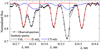 |
Fig. 9 Zr I lines in GIRAFFE spectrum of the target RGB star 23821 (dots) overlaid with the synthetic spectrum (grey solid line) computed using Teff = 4404 K, log g = 1.46, [Fe/H] = -0.76, ?micro = 1.38 km s-1, and ?macro = 4.80 km s-1. Different panels show the environment of Zr I lines located at 612.7475 nm (left), 613.4585 nm (middle), and 614.3252 nm (right). Red and blue solid lines are synthetic profiles of the individual Zr I and CN lines, respectively. |
Impact of CN line blends on the determination of Zr abundances from Zr I lines at different CNO abundances (see Sect. 4.3.1 for details).
Impact of CN line blends on the determination of Zr abundances from Zr II lines at different CNO abundances (see Sect. 4.3.1 for details).
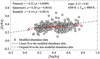 |
Fig. 10 Influence of CN lines on the Zr–Na correlation. To account for the influence of CN blends, the original Zr abundances obtained from Zr I lines in Sect. 3.3.1 were modified by adding a correction which changed linearly from +0.04 dex at [Na/Fe] = 0.10 to −0.04 dex at [Na/Fe] = 0.75. A linear fit to the modified data (filled grey circles) is shown as a red solid line. The black dashed line is linear fit to the non-modified abundances in the [Zr/Fe] – [Na/Fe] plane shown in Fig. 5 (top panel) shifted to match the mean [Zr/Fe] value in the modified data at [Na/Fe] = 0.42. |
4.3.2 Influence of CN blends in the subsample of RGB targets with known C and N abundances
For the second test, we selected a subsample of our target RGB stars for which C and N abundances were determined by Mészáros et al. (2020) using APOGEE-2 spectra. This resulted in a subset of 54 stars. We then determined Zr abundances from the same three Zr I lines as was done in Sect. 3.3.1 but this time using the spectral synthesis methodology to eliminate the influence of CN blends on the determined abundances. For this, we used the SYNTHE package together with the model atmospheres used in the analysis of these stars in Sect. 3, and the CN line list taken from Brooke et al. (2014). The obtained Zr abundances are shown in Fig. 11.
Indeed, the slope in the [Zr/Fe] – [Na/Fe] plane becomes smaller when using Zr abundances obtained by taking the influence of CN lines into account and is equal to ≈+0.12 (Fig. 11). This value is about two times smaller than that obtained using Zr abundances determined with the equivalent width method, of namely ≈0.23 (Sect. 4.2). Part of the difference stems from the fact that for the subsample of 54 RGB stars, the slope in the [Zr/Fe] – [Na/Fe] plane is lower than that obtained for 237 stars, ≈+0.17 vs. ≈+0.23. The rest of the change in the slope, ∆ = +0.05, is caused by CN lines alone, as is seen in Fig. 11.
Thus, the Zr–Na correlation remains prominent when Zr abundances are determined with the line synthesis methodology, that is, by eliminating the influence of CN lines. We obtain p = 0.08 when using this approach on our subsample of 54 RGB stars. If adjusted for the smaller subsample size, this value would become smaller, p = 0.04, and would suggest that the Zr–Na correlation may in fact be real.
4.4 Mean values of Na and Zr abundances in the 1P and 2P stars in 47 Tuc
As the detected Zr–Na correlation is relatively weak, we can also compare mean abundances in the 1P and 2P stars in order to check whether they are indeed statistically different. For this, following Carretta et al. (2009) we classified stars with [Na/Fe] = [[Na/Fe]min, [Na/Fe]min + 0.3] as 1P stars, and those with the higher [Na/Fe] abundance ratios as 2P. In each population, we then computed the mean abundance ratios and the errors of the mean. The obtained results are provided in Table 7.
Using the mean 1P and 2P abundances, we ran the two-sample t-test to verify whether the possible 2P-1P differences are indeed statistically significant. We also did the same test using the modified [Zr/Fe] ratios obtained in Sect. 4.3.1. We did not perform such a test for the subsample of 54 target RGB stars with Zr abundances determined using the line synthesis approach (Sect. 4.3.2) because in this case the sample size was too small for a meaningful comparison of the 2P−1P difference in mean Zr abundance.
When comparing the mean [Na/Fe] abundance ratios in the 1P (N = 93) and 2P (N = 144) stars, the probability of obtaining the t-values by chance is p< 10−15, which supports the notion that the difference that we see between the mean Na abundances in the 1P and 2P stars is real. A similar situation is also seen for the differences in the mean [Zr/Fe] abundance ratios where the p-values obtained using original Zr abundances (Sect. 3.3.1) and abundances adjusted to account for CN blends (Sect. 4.3.1) do not exceed p = 0.07.
Mean [Na/Fe] and [Zr/Fe] abundance ratios in the 1P and 2P stars in 47 Tuc and the corresponding p-values.
4.5 Implications for nucleosynthesis in the GGCs
Taken together, the evidence we find suggests that there may indeed be a statistically significant correlation between [Zr/Fe] and [Na/Fe]. No earlier studies hinted towards the existence of a Zr–Na correlation, either in 47 Tuc or in other GGCs. On the one hand, this is unsurprising given the small number of stars per GGC studied in these papers (N < 14). On the other hand, an analysis of the data obtained by Thygesen et al. (2014) suggests a weak correlation in the [Zr/Fe] – [Na/Fe] plane although the authors did not find it to be statistically significant (see their Fig. A.2). Importantly, abundances from Thygesen et al. (2014) follow the same trend as seen in our data in the [Zr/Fe] – [Na/Fe] plane, even if the mean [Na/Fe] and [Zr/Fe] ratios obtained in the two studies differ slightly (Appendix B.2.4).
Theoretical modelling of s-process element yields shows that Zr may be synthesised both in AGB stars(M ~ 1.5−5 M⊙; Cristallo et al.2015) and massive rotating stars (M ~ 12−25 M⊙, υrot> 150 kms−1; Limongi&Chieffi2018). It is therefore impossible to provide reliable constraints on the possible polluters based on the abundances of Zr alone.
Interestingly, analysis of 106 red horizontal branch (RHB) stars in 47 Tuc by Gratton et al. (2013) revealed a weak but statistically significant correlation in the [Ba/Fe] – [Na/O] plane. In contrast, our recent study of Ba abundance in the same sample of RGB stars as that used in our Zr analysis does not corroborate this finding, as we detect no statistically significant correlation in the [Ba/Fe] – [Na/Fe] plane (Dobrovolskas et al.2021), despite the fact that our target sample was twice as large as that used in Gratton et al. (2013). To the best of our knowledge, there are no other s-process elements with similar correlations detected in 47 Tuc (although there may be hints to such correlations in other Type I GGCs, e.g. Sr-Na and Y–Na relations in M 4, Spite et al. 2016; Villanova & Geisler 2011; but see also D’Orazi et al. 2013).
This evidence is therefore not sufficient to identify the possible enrichment scenario that has operated in this GGC. It is important to stress that existing abundance determinations of other s-process elements are not very helpful here because they show no evidence for correlations with the abundances of light elements, as seen in the case of Zr. Thus, they may reflect abundances of the primordial gas cloud that was enriched prior to the formation of 2P stars. Future investigations of differences between the heavy s-process elements in the 1P and 2P stars of this and other GGCs would therefore be very desirable, especially for large samples of GGC stars as this is critical for a reliable detection of weak correlations between the elemental abundances. In particular, it would be very interesting to check whether such differences also exist for Sr, Y, and other elements of the so-called ‘first s-process peak’ which are synthesised under similar conditions to Zr. In addition, detection of 1P-2P differences for heavier s-process elements in the Ba and Pb peaks may allow more stringent constraints to be placed on the possible polluters, because s-process elements in the different peaks are synthesised under different conditions and in different polluters.
5 Conclusions and outlook
Our analysis of Na and Zr abundances in 237 RGB stars in 47 Tuc suggests the existence of a weak Na–Zr correlation. The data also reveal a small but statistically significant difference between the mean Zr abundances in the 1P and 2P stars, of namely A[Zr/Fe]2P−1P≈ 0.06 dex. Correlation is seen in the [Zr/Fe] – r/rh plane as well, where r is the projected distance from the cluster centre. Although there may be some influence on Zr abundance from blending with CN lines (≤0.08 dex), the residual correlations remain statistically significant when the estimated trends due to CN blends are removed.
If the detected Zr–Na correlation is indeed real, it would indicate that at least some fraction of Zr in 47 Tuc should have been synthesised by the same polluters that enriched 2P stars with light elements. Amongst the potential candidate polluters are AGB stars (M ~ 1.5−5 M⊙Cristallo et al.2015) and/or massive rotating stars (M ~ 12−25 M⊙, υrot>150 kms−1Limongi&Chieffi2018), both of which may synthesise Zr in sizeable amounts. Unfortunately, our Zr data alone do not allow us to distinguish between the pollution scenarios, or to confirm that a combination of them has operated in this GGC. It would therefore be very desirable to investigate whether such 1P-2P differences exist for other s-process elements in this or other GGCs in order to put tighter constraints on the possible polluters and evolutionary scenarios of the GGCs.
Note added in proof
A new study of the s-process element Ce in several GGCs performed by Fernández-Trincado et al.(2021, 2022) seems to suggest the existence of Ce-N and Ce-Al correlations in NGC 6380, Tonantzintla 2 (Ton 2), and perhaps also in 47 Tuc. Together with the Zr-Na correlation in 47 Tuc discussed in our paper, may imply that at least in some GGCs abundances of s-process elements in the 2P stars may be different from those in 1P stars. This, in turn, may indicate that sizeable amounts of s-process elements must have been produced by the potential polluters of the 2P stars.
Acknowledgements
We are very grateful to Tamara Mishenina and Sergey Andrievsky for useful comments during the preparation of the manuscript. Our study has benefited from the activities of the “ChETEC” COST Action (CA16117), supported by COST (European Cooperation in Science and Technology) and from the European Union’s Horizon 2020 research and innovation programme under grant agreement no. 101008324 (ChETEC-INFRA). This work has made use of the VALD database, operated at Uppsala University, the Institute of Astronomy RAS in Moscow, and the University of Vienna.
Appendix A Target RGB stars common to different observing programmes
The list of targets common to the three observing programmes is provided in Table A.1. Amongst them, there are five stars that were observed in all three datasets. This sample of overlapping stars was used to investigate possible systematic shifts in the abundances determined using different datasets (Sect. B.2.1-B.2.3). Abundances obtained using different datasets were averaged. The final sample for the abundance analysis consisted of 237 individual RGB stars.
List of stars common to different observing programmes.
Appendix B Abundance analysis
Abundances of Fe and Zr in the sample of 237 RGB stars were determined using the equivalent width method, assuming LTE in spectral synthesis calculations. In the case of Na, we fitted synthetic line profiles that were computed under the assumption of NLTE. In what follows, we describe some technical aspects of the abundance determination of all three elements, including the line lists, diagnostics of obtained abundances, and a comparison of abundances determined in stars common to several observing programmes.
The list of Fe I and Fe II lines used in the abundance analysis.
Parameters of NaI and Zr I lines used in the abundance analysis.
B.1 Reference abundances in the Sun and Arcturus
To obtain the element-to-iron abundance ratios, [X/Fe], in the sample of RGB stars in 47 Tuc, we determined the reference abundances of Fe, Na, and Zr in the Sun. For this, we used the Kitt Peak Solar Flux atlas (Kurucz et al. 1984) and spectral lines of Fe I, Na I, and Zr I that are identical to those that were used in the analysed RGB targets. Abundances were determined with the 1D hydrostatic ATLAS9 solar model atmosphere that was computed by F. Castelli5 using the solar abundance table from Asplund et al. (2005).
Solar iron abundances were obtained using the equivalent width method. The Fe I line list used for the abundance determination is provided in Table B.1. Atomic line data were taken from the VALD3 database (Ryabchikova et al. 2015). We determined the microturbulence velocity iteratively to obtain zero trend of Fe abundance with the line equivalent width. The obtained solar value, ξmicro= 0.93 km s–1, is in good agreement with the typical values of 0.9–1.0 km s–1 found in other studies (e.g. Doyle et al. 2014). The average solar Fe abundance, A(Fe)⊙ = 7.55 ± 0.01 (σ = 0.06; here ±0.01 is the error of the mean, σ denotes the standard deviation due to line-to-line abundance variation), which was obtained from 29 Fel lines with W <10.5 pm, agrees well with the value of A(Fe)⊙ = 7.52 (σ = 0.06) from Caffau et al. (2011a).
To obtain the reference solar Na abundance, we used the same set of Na I lines and analysis methodology as we used in the analysis of target RGB stars (Sect. B.2.2). Atomic parameters of the Na I lines are listed in Table B.2. We obtained an identical abundance from both Na I lines, A(Na)⊙ = 6.17, which agrees well with A(Na)⊙ = 6.21 ± 0.04 determined by Scott et al. (2015a).
The Zr I lines that were used in the analysis of target RGB stars in 47 Tuc were too weak in the solar spectrum for reliable reference abundance determination. We therefore used solar Zr abundance of A(Zr)⊙ = 2.62 from Caffau et al. (2011b).
We also determined abundances of Fe, Na, and Zr in the atmosphere of Arcturus in order to check whether the abundances obtained from the Fe I, Na I, and Zr I lines used in our study agree with those determined in the earlier studies of Arcturus. As in the case of the Sun, we used the same line lists as those used in the analysis of target RGB stars in 47 Tuc6. The abundances were obtained using the ‘Visible and Near Infrared Atlas of the Arcturus Spectrum 3727-9300 Å’ by Hinkle et al. (2000). We calculated the model atmosphere of Arcturus using the ATLAS9 model atmosphere package and Teff= 4286 K and log g= 1.66 from Ramírez & Allende Prieto (2011), with the solar-scaled chemical composition from Asplund et al. (2005) and α-element enhancement of +0.4 dex.
In case of Arcturus, we determined the microturbulence velocity of ξmicro = 1.78 kms−1 and iron abundance of A(Fe) = 7.03 ± 0.02 (σ = 0.09) or [Fe/H] = -0.52, with both the micro-turbulence velocity and abundance obtained using Fe I lines with W <16 pm. As in the case of the Sun, the mean Fe abundance and microturbulence velocity agrees well with the results obtained in the earlier studies (cf. Ramirez & Allende Prieto 2011; Sheminova 2015).
Abundance of Na in Arcturus was determined in NLTE using the same line list and methodology as utilised in the analysis of RGB stars in 47 Tuc (Sect. B.2.2). We obtained identical Na abundance from both Na I lines, A(Na) = 5.71 or [Na/Fe] = 0.06. This agrees reasonably well with the NLTE estimate of A(Na) = 5.80 derived using a set of 14 NaI lines by Osorio et al. (2020). In LTE, we obtained A(Na) = 5.85 which agrees very well with A(Na) = 5.83 ± 0.03 determined by Ramirez & Allende Prieto (2011) using the two NaI lines utilised in our study (we note that the LTE value obtained by Osorio et al. 2020, A(Na) = 5.91, is noticeably higher than that determined either by us or Ramirez & Allende Prieto 2011).
A Gaussian fit to the observed profiles of Zr I lines in the Arcturus spectrum resulted in the equivalent widths of 5.42 pm, 4.97 pm, and 5.39 pm for the lines located at 612.7475 nm, 613.4585nm, and 614.3252nm, respectively, with the corresponding A(Zr) = 2.05, 1.98, and 1.97. The obtained mean Zr abundance is [Zr/Fe] = -0.10 (r = 0.04). This agrees reasonably well with [Zr/Fe] = 0.01 (r = 0.07) obtained by Worley et al. (2009) from seven Zr I lines.
It is important to note that in the original Kurucz software package (ATLAS9, WIDTH9, SYNTHE) the value of Zr I ionisation potential is set to 6.840 eV (Sbordone et al. 2005). Throughout this study, we used a revised value of 6.634eV from Hackett et al. (1986) which is set as default in the F. Castelli version of the Kurucz’s package7. For Arcturus, this lead to an increase in Zr abundance of +0.29 dex. In case of target RGB stars of 47 Tuc, the corresponding upward change was +0.25 to +0.29 dex at Teff= 4800 K and 4200 K respectively.
B.2 Determination of Fe, Na, and Zr abundance in RGB stars of 47 Tuc: additional tests
B.2.1 Abundance of Fe
As it was described in Sect. 3, for each target RGB star in 47 Tuc, iron abundances were determined using a set of 17 − 28 Fe I lines located at 612.79 − 691.67 nm, with the line lower level excitation potentials spanning the range of 2.18 − 4.61 eV. Atomic data of Fe I and Fe II lines used in the analysis are provided in Table B.1.
There is a very weak dependence of the obtained abundances on ξmicroand Teff (Fig. B.1). However, even between the extreme ends of the effective temperature scale the average difference in Fe abundance is less than 0.05 dex. There are no statistically significant differences between the Fe abundances determined using spectra obtained in different observing programmes (Fig. B.2).
B.2.2 Abundance of Na
As indicated in Sect. 3, an NLTE approach was used to determine Na abundance in 47 Tuc. For this purpose, we used spectral synthesis code MULTI (Carlsson 1986; Korotin et al. 1999) and ATLAS9 model atmospheres, together with the model atom of Na that was exploited in our earlier studies (e.g. Dobrovolskas et al. 2014). Two NaI lines located at 615.4225 and 616.0747nm were used in the abundance analysis (Table B.2).
There is reasonably good agreement between abundances obtained from the two Na I lines, with the differences typically below 0.05 dex (Fig. B.3). While there may be a very weak dependence of the Na abundance on Teff, the differences in Na abundance at the extreme ends of Teff scale do not exceed 0.10dex (Fig. B.4). Furthermore, we find no statistically significant differences between Na abundances determined using spectra obtained in the different observing programmes (Fig. B.5).
B.2.3 Abundance of Zr
As described in Sect. 3.3.1 above, Zr abundance was determined for the target RGB stars using three Zr I lines located at 612.7475, 613.4585, and 614.3252nm (Table B.2) under the assumption of LTE. Examples of the observed and best-fitted Zr I line profiles are shown in Fig. 3.
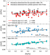 |
Fig. B.1 Abundance of Fe in the target RGB stars, plotted against the microturbulence velocity (top) and effective temperature (bottom). |
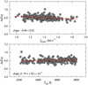 |
Fig. B.2 Differences in the Fe abundances obtained in the target RGB stars that are common to different observing programmes used in this study. In each panel, symbol denotes the mean difference between the A(Fe) values obtained using spectra from the different programmes, s is standard deviation from. |
Abundances obtained from the three Zr I lines agree well, with mean differences in A(Zr) obtained from the individual lines of ≤0.03 dex (Fig. B.6). Also, there are no significant trends of Zr abundance with microturbulence velocity or effective temperature (Fig. B.7). Finally, there are no significant differences between Zr abundances determined using spectra obtained in the different observing programmes (Fig. B.8).
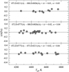 |
Fig. B.3 Differences in the Na abundances obtained from the two NaI lines used in this study. The symbol denotes the mean difference between the A(Na) values obtained using different Na I lines, and c is the standard deviation from. |
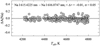 |
Fig. B.4 Abundance of Na in the target RGB stars versus the microtur-bulence velocity (top) and effective temperature (bottom). |
B.2.4 Determination of zirconium abundance using Zr II lines
As discussed in Sect. 3.3.1, Zr abundances in our target RGB stars were determined using three Zr I lines. Unfortunately, all three lines are contaminated with weak CN blends (see Sect. 4.3 which were not taken into account when determining Zr abundances in Sect. 3.3.1.
As discussed in Sect. 3.3.2, several Zr II lines are available for abundance analysis and some of them are free from CN blends (Sect. 4.3). Unfortunately, none of the spectral ranges covering Zr II lines have been observed with GIRAFFE for our target RGB stars. We therefore used the UVES spectra of three stars in our sample obtained by Thygesen et al. (2014) to compare abundances determined from the Zr I and Zr II lines.
The UVES spectra from Thygesen et al. (2014) were obtained in the 580 nm setting, with a resolving power of R=110000. The spectra of the three common stars were taken from the ESO Advanced Data Products archive8. We determined Zr abundances using the same Zr I lines as in the analysis of GIRAFFE spectra (Sect. 3.3.1), as well as Zr I 614.0460nm line (which becomes too weak to be measured reliably in the GIRAFFE spectra for stars with Teff> 4450 K) and three Zr II lines located at 511.2270, 535.0089, and 535.0350nm. Abundances from all lines were obtained by fitting synthetic spectra to the observed line profiles. The main reason for this was that all Zr I and Zr II lines are blended with CN lines (Sect. 4.3). In addition, the 535.0350nm Zr II line is influenced by the weak VII 535.0358 nm and Tl I 535.0456nm lines, while the 511.2270nm Zr II line is affected by the nearby MgH511.2080 nm and CrI 511.2484 nm lines (Fig. B.9); and the Zr I 612.7475nm line is blended with the Fe I 612.7906 nm line (Sect. 3.3.1). Furthermore, Mg abundance influences the opacity of stellar model atmosphere which leads to a slight change in the electron densities and thus in determined Zr abundances. To account for the latter, we used Mg abundances obtained in the three stars by Thygesen et al. (2014). Solar-scaled CN abundances, A(C) = 7.82 and A(N) = 7.22, were used to account for the influence of CN blends, with the CN line data taken from Brooke et al. (2014); see also Sect. 4.3 for more details about the influence of CN blends on the determined Zr abundances.
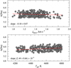 |
Fig. B.5 Differences in the Na abundances obtained in the target RGB stars that are common to different observing programmes. In each panel, the symbol denotes the mean difference between the A(Na) values obtained using spectra from the different programmes, and s is the standard deviation from. |
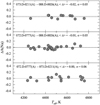 |
Fig. B.6 Differences in the Zr abundances obtained from different Zr I lines used in this study. The symbol denotes the mean difference between the A(Zr) values obtained using different Zr I lines, and c is the standard deviation from. |
 |
Fig. B.7 Abundance of Zr in the target RGB stars versus the microturbulence velocity (top) and effective temperature (bottom). |
For abundance analysis with the UVES spectra we had to modify oscillator strength of the 535.0089 nm line because the VALD3 oscillator strength led to solar Zr abundance that was ~0.28 dex higher than the reference value of A(Zr) = 2.62 from Caffau et al. (2011b, cf. Fig. B.10, left panel); the solar model atmosphere used in the analysis was the same as that used in Sect. B.1. We therefore modified the oscillator strength of this line so that we would obtain A(Zr) = 2.62 from this line in the Kurucz solar spectrum (Fig. B.10, left panel). With the new value of log gf = -0.964, the Zr II 535.0089 nm line gave A(Zr) = 2.17 in Arcturus (Fig. B.10, right panel; the model atmosphere of Arcturus was identical to that used in Sect. B.1). Using A(Fe) = −0.52 determined in Sect. B.1, this gives [Zr/Fe] = +0.07. The latter value agrees well with [Zr/Fe] = +0.01 ± 0.07 determined by Worley et al. (2009) but it is slightly higher than the average Zr abundance in Arcturus that we determined using Zr I lines, [Zr/Fe] = −0.10 (Sect. B.1).
Abundances of Zr in the three stars common to the GIRAFFE (used in this work) and UVES samples (Thygesen et al. 2014), determined from Zr I and Zr II lines in the UVES spectra.
Mean abundances of Fe, Na, and Zr in the three common stars obtained by us from the GIRAFFE and UVES spectra, and those determined by Thygesen et al. (2014) from the same UVES spectra.
 |
Fig. B.8 Differences in the Zr abundances obtained in the target RGB stars that are common to different observing programmes. In each panel, the symbol denotes the mean difference between the A(Zr) values obtained using spectra from the different programmes, s is standard deviation from. |
 |
Fig. B.9 Zr II lines in the UVES spectrum of the target star 20885 (dots) overlaid with the synthetic spectrum (grey solid line) computed using the ATLAS9 model with Teff = 4359 K, log g = 1.41, [Fe/H] = -0.74, [Zr/Fe] = 0.30 dex, ?micro = 1.82 km s-1, ?macro = 3.00 km s-1 and solar-scaled elemental abundances (Grevesse & Sauval 1998). The left panel shows the vicinity of Zr II 511.2270nm line, the right panel that of 535.0089 nm and of 535.0350 nm Zr II lines. Other solid lines are synthetic profiles of individual lines, left panel: Zr II 511.2270nm (red line), MgH 511.2080 nm (green line), CN 511.2360 nm (blue line); right panel: Zr II 535.0089 nm and 535.0350 nm (red line), V II 535.0358 nm (orange line), Tl I 535.0456 nm (cyan line), CN 535.0215 nm (blue line). |
For the three target RGB stars in 47 Tuc that have been observed both in the GIRAFFE and UVES samples, abundances determined from individual Zr I and Zr II lines in the UVES spectra agree to ≤0.06 ex (Table B.3; Fig. B.11). The mean abundances obtained from Zr I lines in the GIRAFFE and UVES spectra agree even better, with the differences being less than 0.03 dex (Table B.4, Fig. B.11).
On average, abundances that we obtained using Zr I lines in the UVES spectra are ~0.10 dex higher than those determined by Thygesen et al. (2014, cf. Table B.4, Fig. B.12). Although there are small differences in the effective temperatures and gravities used in the two studies, they alone cannot account for more than ~0.02 dex of this discrepancy. On average, the microturbulence velocities obtained by Thygesen et al. (2014) are ~0.04 km s−1 lower than those used in our study (Table B.4). This would lead to Zr abundances that are by ~0.1 dex higher than those that would be obtained with our ξmicro values. However, the main difference between the two analyses is that we used an updated ionisation potential for Zr I,6.634 eV from Hackett et al. (1986) instead of the default value of 6.840 eV that is implemented with the older version of Kurucz package (Sect. 3). This alone would lead to our Zr abundances being ~0.29 dex higher. Thus, the latter two effects (working in different directions) would be fully able to account for the difference in Zr abundances obtained by us and Thygesen et al. (2014).
 |
Fig. B.10 Left: Fit of the synthetic Zr II 535.0089 nm line to that observed in the solar spectrum from Kurucz (2005b). The red solid line shows the best fit obtained using the VALD3 oscillator strength, and the blue dashed line is the fit obtained using A(Zr) = 2.62 from Caffau etal. (2011b) and a modified oscillator strength (oscillator strengths and Zr abundances used/determined are indicated in the figure). For the line synthesis we used ?micro = 1.00 km s–1 and ?macro = 3.80 km s–1 from Doyle et al. (2014). Right: Best fit of the synthetic Zr II 535.0089 nm line to that observed in the spectrum of Arcturus from Hinkle et al. (2000). Spectral line synthesis was done using ?micro = 1.70 km s–1 and ftnacro = 5.20 km s–1 from Sheminova (2015). |
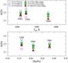 |
Fig. B.11 Abundances of Zr in the three RGB stars common to the GIRAFFE (this study) and UVES samples (Thygesen et al. 2014) determined by us using Zr I and Zr II lines in the GIRAFFE and UVES spectra (Table B.3 and B.4, Sect. B.2.4) and plotted against the effective temperature (top) and [Na/Fe] ratio (bottom). The mean abundances obtained using Zr I lines in the GIRAFFE and UVES spectra are shown by solid red and green triangles, respectively, while the mean abundances obtained from Zr II lines are plotted as green circles; and abundances determined from individual Zr II lines in the UVES spectra are shown as hollow circles. |
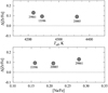 |
Fig. B.12 Differences between Zr abundances determined in this study and those obtained by Thygesen et al. (2014) from Zr I lines in the UVES spectra, plotted against the effective temperature (top) and [Na/Fe] values (bottom). |
B.2.5 Errors in the determined Fe, Na, and Zr abundances
For estimating typical uncertainties in the determined abundances of Fe, Na, and Zr, we followed the procedure described in Černiauskas et al. (2017). With this, we accounted for the following error sources:
The error in abundance due to uncertainty in the determined effective temperature was estimated by computing Teffvalues that were increased and decreased by the amount which corresponded to the uncertainty in determined photometric magnitudes. A conservative estimate of = σ(I) = 0.03 was used, which translated to an uncertainty of ±60 K in the effective temperature. This value was used to estimate abundance uncertainty caused by errors in the determination of Teff.
An abundance error due to uncertainty in the determination of surface gravity, σ(log g) = ±0.2, was obtained by taking into account individual uncertainties in the estimates of Teff, luminosity, and stellar mass.
We used the RMS variation of microturbulence velocity, ±0.2 km s−1, as a representative uncertainty in ξmicro. This value was used to estimate the abundance error due to variationin ξmicro.
-
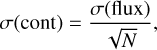
An abundance error due to uncertainties in the continuum determination, σ(cont), was obtained by measuring the continuum flux dispersion, σ(flux), in the wavelength intervals that are located close to the investigated spectral lines and that are line-free:
 (B.1)
(B.1)where N is the number of wavelength points. The resulting error was used to increase and decrease the continuum level, after which the line fitting was done again and the resulting difference in the abundance was taken as the abundance error due to uncertainty in the continuum determination.
To estimate errors in the line profile fitting, we computed RMS variation between the observed and best-fitted line profiles. The line equivalent width was then increased and decreased by this value to obtain the difference in the corresponding abundances of the given element. The latter were used as abundance uncertainties due to errors in the line profile fitting.
Typical Fe abundance measurement errors.
Typical Na abundance measurement errors.
Typical Zr abundance measurement errors.
The final abundance errors were obtained by adding individual error components in quadratures. To obtain abundance errors for our target stars, we selected a subsample of 8 stars for Zr, Na and Fe abundance error estimation, with their effective temperatures distributed evenly over the entire Teff range of 237 RGB targets. Using the prescription above, we determined typical abundance errors of Zr, Na, and Fe for these stars. In this procedure, we assumed median equivalent widths of these lines at the given Teff, i.e. no variation of the line strength was taken into account. The determined abundance errors are provided in Tables B.5-B.7.
Appendix C Statistical significance of possible correlations between the full spatial velocity dispersions and [Na/Fe] and [Zr/Fe] abundance ratios
As in the case of testing the statistical significance of the possible correlations in the abundance–abundance and abundance-radial distance planes, we computed the p-values using Pearson’s, Spearman’s, and Kendall’s correlation coefficients in the </ieq> and </ieq> planes. In the former case, the we obtain p>0.2 which indicates that there is no correlation between the full spatial velocity dispersion and [Na/Fe] ratio. The values obtained for the Spearman’s and Kendall’s coefficients are sufficiently small (p<0.04) to claim the possible existence of a weak correlation in the </ieq> plane, though the p-value obtained for the Pearson’s correlation coefficient is somewhat higher, at p= 0.059.
To further verify the possible existence of the correlation in the </ieq> plane, we tested the statistical significance of differences between the variances of full spatial velocities of individual stars in the 0.1 dex wide [Zr/Fe] and [Na/Fe] abundance bins (Sect. 4 and Fig. 8). This was done using the Levene’s test (Levene 1960; Brown & Forsythe 1974) which was applied to verify the assumption of the null hypothesis that the full spatial velocities in the different [Zr/Fe] and [Na/Fe] abundance bins have equal variances. The obtained p-values were > 0.37 both in the σ(υfull) − [Na/Fe] and σ(υfull) − [Zr/Fe] planes thereby indicating that in both cases the null hypothesis could not be rejected. Based on these results we therefore conclude that there are no statistically significant correlations between the dispersions of full spatial velocities and [Na/Fe] and [Zr/Fe] abundance ratios in the target RGB stars of 47 Tuc.
Appendix D Abundances of Fe, Na, and Zr determined in the target RGB stars in 47 Tuc
Abundances of Fe, Na, and Zr determined in the individual target RGB stars in 47 Tuc (Sect. 3.1, 3.2, and 3.3.1, respectively) are listed in Table D.1, together with the atmospheric parameters of individual targets determined in Sect. 2.1.
References
- Asplund, M., Grevesse, N., & Sauvai, A. J. 2005, ASPC, 336, 25 [NASA ADS] [Google Scholar]
- Asplund, M., Grevesse, N., Sauval A. J., & Scott, P. 2009, ARA&A, 47, 481 [NASA ADS] [CrossRef] [Google Scholar]
- Barklem, P. S., Belyaev, A. K., Dickinson, A. S., et al. 2010, A&A, 519, A20 [NASA ADS] [CrossRef] [EDP Sciences] [Google Scholar]
- Bastian, N., & Lardo, C. 2018, ARA&A, 56, 83 [Google Scholar]
- Baumgardt, H., Hilker, M., Sollima, A., & Bellini, A. 2019, MNRAS, 482, 5138 [Google Scholar]
- Bergbusch, P. A., & Stetson, P. B. 2009, AJ, 138, 1455 [NASA ADS] [CrossRef] [Google Scholar]
- Biemont, E., Grevesse, N., Hannaford, P., & Lowe, R. M. 1981, ApJ, 248, 867 [Google Scholar]
- Bonifacio, P., Pasquini, L., Molaro, P., et al. 2007, A&A, 470, 153 [NASA ADS] [CrossRef] [EDP Sciences] [Google Scholar]
- Brooke, J. S. A., Ram, R. S., Western, C. M., et al. 2014, ApJS, 210, 23 [NASA ADS] [CrossRef] [Google Scholar]
- Brown, M. B., & Forsythe, A. B. 1974, J. Am. Stat. Assoc., 69, 364 [CrossRef] [Google Scholar]
- Caffau, E., Ludwig, H.-G., Steffen, M., Freytag, B., & Bonifacio, P. 2011, Sol. Phys., 268, 255 [Google Scholar]
- Caffau, E., Faraggiana, R., Ludwig, H.-G., Bonifacio, P., & Steffen, M. 2011, Astron. Nachr., 332, 128 [NASA ADS] [CrossRef] [Google Scholar]
- Carlsson, M. 1986, Upps. Astron. Obs. Rep., 33, 33 [Google Scholar]
- Carretta, E., Gratton, R. G., Lucatello, S., Bragaglia, A., & Bonifacio, P. 2005, A&A, 433, 597 [NASA ADS] [CrossRef] [EDP Sciences] [Google Scholar]
- Carretta, E., Bragaglia, A., Gratton, R. G., et al. 2009, A&A, 505, 117 [NASA ADS] [CrossRef] [EDP Sciences] [Google Scholar]
- Cerniauskas, A., Kucinskas, A., Klevas, J., et al. 2017, A&A, 604, A35 [NASA ADS] [CrossRef] [EDP Sciences] [Google Scholar]
- Cordero, M. J., Pilachowski, C. A., Johnson, C. I., et al. 2014, ApJ, 780, 94 [Google Scholar]
- Cordero, M. J., Hansen, C. J., Johnson, C. I., & Pilachowski, C. A. 2015, ApJ, 808, L10 [NASA ADS] [CrossRef] [Google Scholar]
- Cristallo, S. 2018, EPJ Web Conf., 184, 01004 [NASA ADS] [CrossRef] [EDP Sciences] [Google Scholar]
- Cristallo, S., Straniero, O., Piersanti, L., & Gobrecht, D. 2015, ApJS, 219, 40 [Google Scholar]
- D’Antona, F., Vesperini, E., D’Ercole, A., et al. 2016, MNRAS, 458, 2122 [Google Scholar]
- Decressin, T., Charbonnel, C., Siess, L., et al. 2007, A&A, 505, 727 [Google Scholar]
- Denisenkov, P. A., & Hartwick, F. D. A. 2014, MNRAS, 437, L21 [NASA ADS] [CrossRef] [Google Scholar]
- Dobrovolskas, V., Kucinskas, A., Bonifacio, P., et al. 2014, A&A, 565, A121 [NASA ADS] [CrossRef] [EDP Sciences] [Google Scholar]
- Dobrovolskas, V., Kolomiecas, E., Kucinskas, A., & Korotin, S. 2021, A&A, 656, A67 [NASA ADS] [CrossRef] [EDP Sciences] [Google Scholar]
- Doyle, A. P., Davies, G. R., Smalley, B., Chaplin, W. J., & Elsworth, Y. 2014, MNRAS, 444, 3592 [Google Scholar]
- D’Orazi, V. D., Campbell, S. W., Lugaro, M., et al. 2013, MNRAS, 433, 366 [CrossRef] [Google Scholar]
- Fernández-Trincado, J. G., Beers, T. C., Barbuy, B., et al. 2021, ApJ, 918, L9 [CrossRef] [Google Scholar]
- Fernández-Trincado, J. G., Villanova, S., Geisler, D., et al. 2022, A&A, 658, A116 [NASA ADS] [CrossRef] [EDP Sciences] [Google Scholar]
- Gaia Collaboration (Brown A. G. A., et al.) 2021, A&A, 649, A1 [NASA ADS] [CrossRef] [EDP Sciences] [Google Scholar]
- Gieles, M., Charbonnel, C., Krause, M. G. H., et al. 2018, MNRAS, 478, 2461 [Google Scholar]
- Gratton, R. G., Lucatello, S., Sollima, A., et al. 2013, A&A, 549, A41 [NASA ADS] [CrossRef] [EDP Sciences] [Google Scholar]
- Grevesse, N., & Sauval, A. J. 1998, Space Sci. Rev., 85, 161 [Google Scholar]
- Grevesse, N., Scott, P., Asplund, M., & Sauval, A. J. 2015, A&A, 573, A27 [CrossRef] [EDP Sciences] [Google Scholar]
- Hackett, P. A., Humphries, M. R., Mitchell, S. A., & Rayner, D. M. 1986, J. Chem. Phys., 85, 3194 [NASA ADS] [CrossRef] [Google Scholar]
- Hinkle, K., Wallace, L., Valenti, J., & Harmer, D. 2000, Visible and Near Infrared Atlas of the Arcturus Spectrum 3727-9300 Å, eds. K. Hinkle, L. Wallace, J. Valenti, & D. Harmer (San Francisco: ASP), 200 [Google Scholar]
- Igenbergs, K., Schweinzer, J., Bray, I., Bridi, D., & Aumayr, F. 2008, Atomic Data Nuclear Data Tables, 94, 981 [NASA ADS] [CrossRef] [Google Scholar]
- Kim, Y.-C., Demarque, P., Yi, S. K., & Alexander, D. R. 2002, ApJS, 143, 499 [Google Scholar]
- Korotin, S. A., Andrievsky, S. M., & Luck, R. E. 1999, A&A, 351, 168 [NASA ADS] [Google Scholar]
- Kucinskas, A., Dobrovolskas, V., & Bonifacio, P. 2014, A&A, 568, L4 [NASA ADS] [CrossRef] [EDP Sciences] [Google Scholar]
- Kurucz, R. L. 1993, ATLAS9 Stellar Atmosphere Programs and 2 km/s Grid, CD-ROM No.13, Cambridge, Mass. [Google Scholar]
- Kurucz, R. L. 2005, Mem. S. A. It. Suppl., 8, 14 [NASA ADS] [Google Scholar]
- Kurucz, R. L. 2005, Mem. S. A. It. Suppl., 8, 189 [Google Scholar]
- Kurucz, R. L., Furenlid, I., Brault, J., & Testerman, L. 1984, Solar Flux Atlas from 296 to 1300 nm (Sunspot, New Mexico: National Solar Observatory) [Google Scholar]
- Levene, H. 1960, Robust tests for equality of variances, in ed. I. Olkin, Contributions to Probability and Statistics (Palo Alto: Stanford University Press), 278 [Google Scholar]
- Limongi, M., & Chieffi, A. 2018, ApJS, 237, 13 [NASA ADS] [CrossRef] [Google Scholar]
- Marino, A. F., Milone, A. P., Karakas, A. I., et al. 2015, MNRAS, 450, 815 [NASA ADS] [CrossRef] [Google Scholar]
- Marino, A. F., Milone, A. P., Renzini, A., et al. 2019, MNRAS, 487, 3815 [CrossRef] [Google Scholar]
- Mészáros, S., Masseron, T., García-Hernández, D. A., et al. 2020, MNRAS, 492, 1641 [Google Scholar]
- Milone, A. P., Marino, A. F., Mastrobuono-Battisti, A., & Lagioia, E. P. 2018, MNRAS, 479, 5005 [NASA ADS] [CrossRef] [Google Scholar]
- Mucciarelli, A., Bellazzini, M., & Massari, D. 2021, A&A, 653, A90 [NASA ADS] [CrossRef] [EDP Sciences] [Google Scholar]
- Osorio, Y., Allende Prieto, C., Hubeny, I., Mészáros, Sz., & Shetrone, M. 2020, A&A, 637, A80 [NASA ADS] [CrossRef] [EDP Sciences] [Google Scholar]
- Pasquini, L., Bonifacio, P., Molaro, P., et al. 2005, A&A, 441, 549 [NASA ADS] [CrossRef] [EDP Sciences] [Google Scholar]
- Prantzos, N., Abia, C., Limongi, M., Chieffi, A., & Cristallo, S. 2018, MNRAS, 476, 3432 [Google Scholar]
- Ramírez, I., & Meléndez, J. 2005, ApJ, 626, 465 [Google Scholar]
- Ramírez, I., & Allende Prieto, C. 2011, ApJ, 743, 135 [Google Scholar]
- Ryabchikova, T., Piskunov, N., Kurucz, R. L., et al. 2015, Phys. Scr., 90, 054005 [Google Scholar]
- Sbordone, L. 2005, Mem. Soc. Astron. It., 8, 61 [Google Scholar]
- Scott, P., Asplund, M., Grevesse, N., Bergemann, M., & Sauval, A. J. 2015a, A&A, 573, A25 [NASA ADS] [CrossRef] [EDP Sciences] [Google Scholar]
- Scott, P., Asplund, M., Grevesse, N., Bergemann, M., & Sauval, A. J. 2015b, A&A, 573, A26 [NASA ADS] [CrossRef] [EDP Sciences] [Google Scholar]
- Sheminova, V. A. 2015, Kinemat. Phys. Celest. Bodies, 31, 172 [NASA ADS] [CrossRef] [Google Scholar]
- Shen, Z.-X., Bonifacio, P., Pasquini, L., et al. 2010, A&A, 524, L2 [NASA ADS] [CrossRef] [EDP Sciences] [Google Scholar]
- Spite, M., Spite, F., Gallagher, A. J., et al. 2016, A&A, 594, A79 [NASA ADS] [CrossRef] [EDP Sciences] [Google Scholar]
- Thygesen, A. O., Sbordone, L., Andrievsky, S., et al. 2014, A&A, 572, A108 [NASA ADS] [CrossRef] [EDP Sciences] [Google Scholar]
- Tody, D. 1986, Proc. SPIE, 627, 733 [NASA ADS] [CrossRef] [Google Scholar]
- Trager, S. C., Djorgovski, S., & King, I. R. 1993, ASPC, 50, 347T [NASA ADS] [Google Scholar]
- Villanova, S., & Geisler, D. 2011, A&A, 535, A31 [NASA ADS] [CrossRef] [EDP Sciences] [Google Scholar]
- Wang, Y., Primas, E., Charbonnel, C., et al. 2017, A&A, 607, A135 [NASA ADS] [CrossRef] [EDP Sciences] [Google Scholar]
- Worley, C. C., Cottrell, P. L., Freeman, K. C., & Wylie-de Boer, E. C. 2009, MNRAS, 400, 1039 [NASA ADS] [CrossRef] [Google Scholar]
- Worley, C. C., Cottrell, I., McDonald, K. C., & van Loon, J. Th. 2010, MNRAS, 402, 2060 [NASA ADS] [CrossRef] [Google Scholar]
- Wylie, E. C., Cottrell, P. L., Sneden, C. A., & Lattanzio, J. C. 2006, ApJ, 649, 248 [NASA ADS] [CrossRef] [Google Scholar]
- Yong, D., Meléndez, J., Grundahl, F., et al. 2013, MNRAS, 434, 3542 [NASA ADS] [CrossRef] [Google Scholar]
Version 2 from http://www.astro.yale.edu/demarque/yyiso.html
As was already mentioned in Sect. 2.1, typically, only 2-3 Fe II lines could be measured reliably in the target star spectra. For this reason, we did not determine stellar gravities using the assumption of ionization equilibrium.
Note that the Fe I line sets used to determine Fe abundances in the Sun, Arcturus, and RGB stars in 47 Tuc were not identical but individual lines were always selected from the list in Table B.1.
All Tables
Impact of HFS on the determination of Zr abundance from the Zr I lines used in this study.
Minimum, maximum, and mean Fe, Na, and Zr abundance ratios determined in the sample of 237 RGB stars in 47 Tuc.
Pearson, Spearman and Kendall correlation coefficients and the corresponding p-values in the [Zr/Fe]–[Na/Fe] and abundance–distance planes.
Impact of CN line blends on the determination of Zr abundances from Zr I lines at different CNO abundances (see Sect. 4.3.1 for details).
Impact of CN line blends on the determination of Zr abundances from Zr II lines at different CNO abundances (see Sect. 4.3.1 for details).
Mean [Na/Fe] and [Zr/Fe] abundance ratios in the 1P and 2P stars in 47 Tuc and the corresponding p-values.
Abundances of Zr in the three stars common to the GIRAFFE (used in this work) and UVES samples (Thygesen et al. 2014), determined from Zr I and Zr II lines in the UVES spectra.
Mean abundances of Fe, Na, and Zr in the three common stars obtained by us from the GIRAFFE and UVES spectra, and those determined by Thygesen et al. (2014) from the same UVES spectra.
All Figures
|
Fig. 1 Atmospheric parameters of the target RGB stars. Stars observed in different programmes are shown in different symbols and colours: orange triangles – 072.D-0777(A), grey circles – 073.D-0211(A), blue diamonds – 088.D-0026(A). The Yonsei-Yale isochrone of 12 Gyr and [M/H] = -0.68, and [a/Fe] = +0.4 is shown for comparison as a red solid line (Kim et al. 2002). |
| In the text | |
|
Fig. 2 Proper motions of the target RGB stars from the Gaia EDR3 catalogue (Gaia Collaboration 2021). Identifications of non-member stars are shown next to the symbols. The region that encloses motions falling within 1.5 mas yr-1 from the mean cluster proper motion is marked by a orange circle. Stars falling outside this region were rejected from the abundance analysis. Zoomed-in region marked by a square is shown in the top right corner. |
| In the text | |
|
Fig. 3 Observed (dots) and best-fitted synthetic profiles of the Na I (NLTE) and Zr I (LTE) lines (red solid lines) in the GIRAFFE spectra of two RGB stars in 47 Tuc: Na-rich (23175, 2P, top row) and Na-poor (R266, 1P, bottom row). Identification numbers of each star, their atmospheric parameters, and the determined Na and Zr abundances are provided in the leftmost panels of each row. The blue lines show synthetic spectrum computed with A(Zr) = 0 to show the possible influence of CN and other blends (further discussed in Sect. 4.3.). |
| In the text | |
|
Fig. 4 Microturbulence velocity in the target RGB stars, ?micro, versus the effective temperature of individual stars. |
| In the text | |
|
Fig. 5 [Zr/Fe] ratios in the sample of 237 RGB stars in 47 Tuc. Top panel: [Zr/Fe] versus [Na/Fe] ratios. Middle and bottom panels, respectively: [Zr/Fe] and [Na/Fe] ratios versus projected distance from the cluster centre, r/rh. Linear least-square best fits are shown as solid lines, fit parameters, correlation coefficients, and the p-values are provided in each individual panel. Typical errors of the individual abundance measurements are indicated in the top panel. |
| In the text | |
|
Fig. 6 [Zr/Fe] – [Na/Fe] plots for stars divided into bins of ?Teff = 100 K (N is the number of stars in each bin). Values of different correlation coefficients and the corresponding p-values are provided for each temperature bin. |
| In the text | |
|
Fig. 7 Full spatial velocities of 237 RGB stars in 47 Tuc versus their [Na/Fe] and [Zr/Fe] ratios (top and bottom, respectively). |
| In the text | |
|
Fig. 8 Dispersions of full spatial velocities of the target RGB stars computed in non-overlapping [Zr/Fe] (top panel) and [Na/Fe] (bottom panel) abundance bins of 0.1 dex. Solid lines are linear least-square fits and the number of stars in each abundance bin is indicated next to each data point. Indicated are the p-values that were obtained using different methods (including the Levene’s test, see Appendix C), and error bars were computed using the bootstrapping technique. |
| In the text | |
|
Fig. 9 Zr I lines in GIRAFFE spectrum of the target RGB star 23821 (dots) overlaid with the synthetic spectrum (grey solid line) computed using Teff = 4404 K, log g = 1.46, [Fe/H] = -0.76, ?micro = 1.38 km s-1, and ?macro = 4.80 km s-1. Different panels show the environment of Zr I lines located at 612.7475 nm (left), 613.4585 nm (middle), and 614.3252 nm (right). Red and blue solid lines are synthetic profiles of the individual Zr I and CN lines, respectively. |
| In the text | |
|
Fig. 10 Influence of CN lines on the Zr–Na correlation. To account for the influence of CN blends, the original Zr abundances obtained from Zr I lines in Sect. 3.3.1 were modified by adding a correction which changed linearly from +0.04 dex at [Na/Fe] = 0.10 to −0.04 dex at [Na/Fe] = 0.75. A linear fit to the modified data (filled grey circles) is shown as a red solid line. The black dashed line is linear fit to the non-modified abundances in the [Zr/Fe] – [Na/Fe] plane shown in Fig. 5 (top panel) shifted to match the mean [Zr/Fe] value in the modified data at [Na/Fe] = 0.42. |
| In the text | |
|
Fig. B.1 Abundance of Fe in the target RGB stars, plotted against the microturbulence velocity (top) and effective temperature (bottom). |
| In the text | |
|
Fig. B.2 Differences in the Fe abundances obtained in the target RGB stars that are common to different observing programmes used in this study. In each panel, symbol denotes the mean difference between the A(Fe) values obtained using spectra from the different programmes, s is standard deviation from. |
| In the text | |
|
Fig. B.3 Differences in the Na abundances obtained from the two NaI lines used in this study. The symbol denotes the mean difference between the A(Na) values obtained using different Na I lines, and c is the standard deviation from. |
| In the text | |
|
Fig. B.4 Abundance of Na in the target RGB stars versus the microtur-bulence velocity (top) and effective temperature (bottom). |
| In the text | |
|
Fig. B.5 Differences in the Na abundances obtained in the target RGB stars that are common to different observing programmes. In each panel, the symbol denotes the mean difference between the A(Na) values obtained using spectra from the different programmes, and s is the standard deviation from. |
| In the text | |
|
Fig. B.6 Differences in the Zr abundances obtained from different Zr I lines used in this study. The symbol denotes the mean difference between the A(Zr) values obtained using different Zr I lines, and c is the standard deviation from. |
| In the text | |
|
Fig. B.7 Abundance of Zr in the target RGB stars versus the microturbulence velocity (top) and effective temperature (bottom). |
| In the text | |
|
Fig. B.8 Differences in the Zr abundances obtained in the target RGB stars that are common to different observing programmes. In each panel, the symbol denotes the mean difference between the A(Zr) values obtained using spectra from the different programmes, s is standard deviation from. |
| In the text | |
|
Fig. B.9 Zr II lines in the UVES spectrum of the target star 20885 (dots) overlaid with the synthetic spectrum (grey solid line) computed using the ATLAS9 model with Teff = 4359 K, log g = 1.41, [Fe/H] = -0.74, [Zr/Fe] = 0.30 dex, ?micro = 1.82 km s-1, ?macro = 3.00 km s-1 and solar-scaled elemental abundances (Grevesse & Sauval 1998). The left panel shows the vicinity of Zr II 511.2270nm line, the right panel that of 535.0089 nm and of 535.0350 nm Zr II lines. Other solid lines are synthetic profiles of individual lines, left panel: Zr II 511.2270nm (red line), MgH 511.2080 nm (green line), CN 511.2360 nm (blue line); right panel: Zr II 535.0089 nm and 535.0350 nm (red line), V II 535.0358 nm (orange line), Tl I 535.0456 nm (cyan line), CN 535.0215 nm (blue line). |
| In the text | |
|
Fig. B.10 Left: Fit of the synthetic Zr II 535.0089 nm line to that observed in the solar spectrum from Kurucz (2005b). The red solid line shows the best fit obtained using the VALD3 oscillator strength, and the blue dashed line is the fit obtained using A(Zr) = 2.62 from Caffau etal. (2011b) and a modified oscillator strength (oscillator strengths and Zr abundances used/determined are indicated in the figure). For the line synthesis we used ?micro = 1.00 km s–1 and ?macro = 3.80 km s–1 from Doyle et al. (2014). Right: Best fit of the synthetic Zr II 535.0089 nm line to that observed in the spectrum of Arcturus from Hinkle et al. (2000). Spectral line synthesis was done using ?micro = 1.70 km s–1 and ftnacro = 5.20 km s–1 from Sheminova (2015). |
| In the text | |
|
Fig. B.11 Abundances of Zr in the three RGB stars common to the GIRAFFE (this study) and UVES samples (Thygesen et al. 2014) determined by us using Zr I and Zr II lines in the GIRAFFE and UVES spectra (Table B.3 and B.4, Sect. B.2.4) and plotted against the effective temperature (top) and [Na/Fe] ratio (bottom). The mean abundances obtained using Zr I lines in the GIRAFFE and UVES spectra are shown by solid red and green triangles, respectively, while the mean abundances obtained from Zr II lines are plotted as green circles; and abundances determined from individual Zr II lines in the UVES spectra are shown as hollow circles. |
| In the text | |
|
Fig. B.12 Differences between Zr abundances determined in this study and those obtained by Thygesen et al. (2014) from Zr I lines in the UVES spectra, plotted against the effective temperature (top) and [Na/Fe] values (bottom). |
| In the text | |
Current usage metrics show cumulative count of Article Views (full-text article views including HTML views, PDF and ePub downloads, according to the available data) and Abstracts Views on Vision4Press platform.
Data correspond to usage on the plateform after 2015. The current usage metrics is available 48-96 hours after online publication and is updated daily on week days.
Initial download of the metrics may take a while.