| Issue |
A&A
Volume 659, March 2022
|
|
|---|---|---|
| Article Number | A180 | |
| Number of page(s) | 8 | |
| Section | The Sun and the Heliosphere | |
| DOI | https://doi.org/10.1051/0004-6361/202142940 | |
| Published online | 24 March 2022 | |
Scaling properties of magnetic field fluctuations in the quiet Sun
1
Istituto Nazionale di Geofisica e Vulcanologia, Via di Vigna Murata 605, 00143 Roma, Italy
e-mail: This email address is being protected from spambots. You need JavaScript enabled to view it.
2
Institute for Space Astrophysics and Planetology (IAPS), Via del Fosso del Cavaliere 100, 00133 Roma, Italy
3
Department of Physics, University of Rome Tor Vergata, Via della Ricerca Scientifica 1, 00133 Roma, Italy
Received:
17
December
2021
Accepted:
14
January
2022
Abstract
Context. The study of the dynamic properties of small-scale magnetic fields in the quiet photosphere is important for several reasons: (i) it allows us to characterise the dynamic regime of the magnetic field and points out some aspects that play a key role in turbulent convection processes; (ii) it provides details of the processes and the spatial and temporal scales in the solar photosphere at which the magnetic fields emerge, vary, and eventually decay; and (iii) it provides physical constraints on models, improving their ability to reliably represent the physical processes occurring in the quiet Sun.
Aims. We aim to characterise the dynamic properties of small-scale magnetic fields in the quiet Sun through the investigation of the scaling properties of magnetic field fluctuations.
Methods. To this end, we applied the structure functions analysis, which is typically used in the study of complex systems (e.g. in approaching turbulence). In particular, we evaluated the so-called Hölder-Hurst exponent, which points out the persistent nature of magnetic field fluctuations in the field of view targeted at a whole supergranule in the disc centre.
Results. We present the first map of a solar network quiet region as represented by the Hölder-Hurst exponent. The supergranular boundary is characterised by persistent magnetic field fluctuations, which indicate the occurrence of longer-memory processes. On the contrary, the regions inside the supergranule are characterised by antipersistent magnetic field fluctuations, which suggest the occurrence of physical processes with a short memory. Classical Kolmogorov homogeneous and isotropic turbulence, for instance, belongs to this class of processes. The obtained results are discussed in the context of the current literature.
Key words: Sun: photosphere / Sun: magnetic fields
© ESO 2022
1. Introduction
The reasons for studying the dynamic properties of small-scale magnetic fields in the quiet photosphere are manifold. Firstly, magnetic fields provide an opportunity to probe some aspects inherent to turbulent convection (see, e.g. Abramenko et al. 2011; Lepreti et al. 2012; Giannattasio et al. 2013, 2014a,b; Giannattasio et al. 2019; Abramenko 2014, 2017; Del Moro et al. 2015; Caroli et al. 2015; Chian et al. 2019; Giannattasio & Consolini 2021) and energy propagation to the upper atmospheric layers (see, e.g. Viticchié et al. 2006; Jefferies et al. 2006; Tomczyk et al. 2007; De Pontieu et al. 2007; Chae & Sakurai 2008; Stangalini et al. 2014, 2015, 2017; Stangalini 2014; Rouppe van der Voort et al. 2016; Gošić et al. 2018; Bellot Rubio & Orozco Suárez 2019; Rajaguru et al. 2019; Keys et al. 2019, 2020; Guevara Gómez et al. 2021; Jess et al. 2021) that cannot be addressed otherwise from an observational point of view. Secondly, they allow us to constrain the available energy in the quiet Sun and infer some details of the processes that amplify and organise them from subgranular to supergranular scales (see, e.g. November 1980; Roudier et al. 1998; Berrilli et al. 1999, 2002, 2004; Berrilli et al. 2005, 2013, 2014; Consolini et al. 1999; Getling & Brandt 2002; Rast 2002; Del Moro 2004; Del Moro et al. 2004; Getling 2006; Nesis et al. 2006; Centeno et al. 2007; Brandt & Getling 2008; de Wijn et al. 2008; Yelles Chaouche et al. 2011; Orozco Suárez et al. 2012; Giannattasio et al. 2018, 2020; Requerey et al. 2018). Thirdly, their study provides important constraints for theoretical models and/or models implemented in simulations of the photospheric layer (see, e.g. Stein & Nordlund 1998, 2001; Cattaneo et al. 2003; Vögler et al. 2005; Rempel et al. 2009; Shelyag et al. 2011; Beeck et al. 2012; Rempel 2014; Danilovic et al. 2015; Khomenko et al. 2017). All these aspects coalesce, advancing our knowledge of the processes capable of accumulating, transporting, and eventually dissipating the enormous amount of energy available in the photosphere of the quiet Sun.
In the last few decades, the dynamic properties of the quiet Sun have been thoroughly investigated using a range of substantially different techniques, allowing us to elaborate a consistent picture of the photospheric dynamics by approaching the problem from different points of view. Particularly interesting and promising are the studies involving the tracking of small-scale magnetic fields in the quiet photosphere. Such investigations reveal features that still cannot be captured by theoretical models and/or simulations because of the complexity of the system and the simultaneous coupling of a wide range of spatial and temporal scales. These studies are based on the hypothesis that magnetic fields are passively transported by the plasma flow and provide a characterisation of advection and diffusion processes in the quiet photosphere from granular to supergranular scales (see, e.g. Wang 1988; Berger et al. 1998; Cadavid et al. 1998, 1999; Hagenaar et al. 1999; Lawrence et al. 2001; Sánchez Almeida et al. 2010; Abramenko et al. 2011; Manso Sainz et al. 2011; Lepreti et al. 2012; Giannattasio et al. 2013, 2014a,b; Giannattasio et al. 2019; Keys et al. 2014; Caroli et al. 2015; Del Moro et al. 2015; Yang et al. 2015a,b; Roudier et al. 2016; Abramenko 2017; Kutsenko et al. 2018; Agrawal et al. 2018; Giannattasio & Consolini 2021). These studies reveal an anomalous scaling of magnetic field transport with a superdiffusive character consistent with a Levy walk inside supergranules and a more Brownian-like motion in their boundary. This has provided constraints on the magnetic flux emergence and evolution that models have to consider in order to fully explain the dynamics governing these environments. At the same time, the scaling laws affecting magnetic fields in the quiet Sun are crucial to understanding how such fields vary with scale size, despite the small scales at which dissipation occurs still being inaccessible with the currently available observations (see, e.g. Lawrence et al. 1994; Stenflo 2012, and references therein). For example, in the milestone work by Stenflo (2012), the spectrum of magnetic flux density in the quiet Sun was found to be consistent with a Kolmogorov power-law scaling. The scale at which scale invariance is broken lies below the current resolution limit. This latter author argued that the collapse of magnetic fields in Kilogauss flux tubes injects energy that is expected to cascade down because of the flux decay occurring via interchange instability, and to fragment into weaker ‘hidden’ fields at smaller scales (down to ∼10 km). As far as we know, no other studies have focused on the scaling properties characterising the magnetic fields in a quiet Sun region within a range of spatial and temporal scales from (sub)granular to supergranular in the time domain. In this work, for the first time we apply the structure function analysis typical of complex systems (Frisch 1995) to fill this gap. This approach complements the studies based on feature tracking mentioned above. The main difference is that, while in those works statistical properties of the photospheric plasma flows are investigated via the transport of small-scale magnetic fields in a frozen-in condition, here we directly study the magnetic field variations emerging from magnetogram time-series. The paper is organised as follows. Section 2 describes the data set used and the analysis techniques applied. Section 3 describes the obtained results, while Sect. 4 is devoted to their discussion in the light of current literature. Finally, in Sect. 5, we present our conclusions and present future perspectives.
2. Observations and data analysis
2.1. The data set
The data set analysed in this work was acquired by the Solar Optical Telescope on board the Hinode mission (Kosugi et al. 2007; Tsuneta et al. 2008) on 2010 November 2 in the framework of the Hinode Operation Plan 151 entitled ‘Flux replacement in the photospheric network and internetwork’. The data set consists of a time-series of 959 simultaneous line-of-sight (LoS) magnetograms and dopplergrams with 90 s cadence, which corresponds to a time range of ∼24 h without interruption, starting at 08:00:42 UT and targeted at a quiet region in the disc centre. Magnetograms were obtained from the Narrowband Filter Imager using the signal acquired in the wings of the spectral line Na I D, i.e. at 589.6 ± 1.6 nm. Data were then binned to a pixel size of 0.16 arcsec (corresponding to a linear size of ∼116 km in the solar photosphere) and a spatial resolution of ∼0.3 arcsec. The field of view (FoV) covers an area of 443 × 456 pixel2, corresponding to a region of ∼70 arcsec (about 50 Mm) in width. The noise level is ∼4 G for single magnetograms, and was computed as the root mean square value in a sub-FoV free of magnetic signal convolved with a 3 × 3 Gaussian kernel (see Gošić et al. 2014, for further details). Magnetograms were coaligned, trimmed to the same FoV, and filtered out for oscillations at 3.3 mHz in order to remove the effects of acoustic oscillations (Gošić et al. 2014, 2016). The peculiarity of this data set is that the FoV encloses an entire supergranule, which is clearly visible when combining the information from both the mean magnetogram and horizontal velocity averaged over ∼24 h (see, e.g. Giannattasio et al. 2014a, 2018). Such a long and uninterrupted observation of an entire supergranule at high resolution and free from seeing effects makes this data set unique and particularly suitable for studying the dynamic properties of magnetic fields in the quiet Sun.
In the left panel of Fig. 1, we show the first frame of the magnetogram time-series, i.e. that acquired on 2010 November 2 at 08:00:42 UT, saturated between −600 G and 600 G. In this frame, the magnetic strength ranges between ≃−1133 G and ≃927 G. In the right panel of the same figure, we show the mean magnetogram averaged over the entire time-series (∼24 h) saturated between −300 G and 300 G. The arrows point to two pixels belonging to inner (A, green arrow) and boundary (B, red arrow) regions of the supergranule. These are used below to make comparisons between these environments. Figure 2 shows the mean dopplergram averaged over the entire time-series and saturated between −0.10 km s−1 and 0.10 km s−1. The vertical velocity in the FoV ranges between −0.12 km s−1 and 0.19 km s−1. In particular, positive values refer to downflowing plasma revealed via the redshift of the Na absorption line, while negative values refer to upflowing plasma revealed via the blueshift of the Na absorption line.
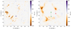 |
Fig. 1. Left panel: first frame of the magnetogram time-series acquired on 2010 November 2 at 08:00:42 UT, saturated between −600 G and 600 G; Right panel: mean magnetogram averaged over the entire magnetogram time-series (∼24 h) saturated between −300 G and 300 G. The green and red arrows point to two pixels belonging to inner (A) and boundary (B) regions of the supergranule, respectively. |
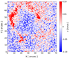 |
Fig. 2. Mean plasma vertical velocity over the entire dopplergram time-series saturated between −0.1 km s−1 and 0.1 km s−1. Positive (red) velocities indicate redshifted downflowing plasma, while negative (blue) velocities indicate blueshifted upflowing plasma. |
2.2. Structure functions and the Hölder-Hurst exponent
A reliable way to characterise the magnetic field variations associated with small-scale magnetic fields is to investigate their scaling properties. This can be done using techniques involving the structure functions, which are commonly used in many fields of research involving complex systems (see, e.g. Frisch 1995, for applications in the study of turbulent phenomena). In the context of solar magnetic fields, structure function analysis in the spatial domain was successfully applied by Abramenko et al. (2002) for example to investigate active regions, and by Abramenko (2014) to investigate quiet Sun areas. Here, we focus on the application of the same technique in the time domain. In particular, we study the persistent character of magnetic field variations, that is, the tendency for positive increments to be followed by positive (persistency) or negative (antipersistency) increments and vice versa. As the region studied is close to the centre of the solar disc, the LoS component of the magnetic field can be equated to the field component normal to the solar surface, namely Bn. Hereafter, we refer to B and Bn interchangeably. Given a one-dimensional signal, such as the pixel-by-pixel time variation of magnetic field as retrieved from the magnetogram time-series, namely B(t), the qth-order generalised structure function, Sq, on the timescale τ, is defined as
 (1)
(1)
where the angular brackets indicate the ensemble average of all the possible pairs of increments separated by the time τ, which identifies the scale of interest. In our case, the lowest accessible scale is τ = 90 s, corresponding to the time cadence of magnetograms. If the signal B(t) is stationary in some sense and its fluctuations are scale invariant, the structure functions satisfy the scaling law
 (2)
(2)
where ξ(q) is the scaling index or scaling exponent associated with Sq. For signals exhibiting a simple (monofractal) scaling, meaning that a single scaling index is capable of describing the variations of B(t) at all scales and everywhere in the FoV, the relation ξ(q)=Cq holds with C ∈ ℝ. However, in general, ξ is non-linear in q and a single scaling index is not sufficient to characterise the scaling properties of the signal. In this case, we are in the presence of a multifractal scaling, which may, for example, be the signature of the occurrence of intermittency in the inertial range of turbulent media (Frisch 1995).
Particularly interesting is the first-order structure function, S1(τ), and the associated scaling index ξ(1). This quantity allows us to describe the pixel-by-pixel temporal structure of the magnetic field variations and their scaling at different scales of observation, τ. In particular, the quantity ξ(1) can be reasonably identified with the Hölder-Hurst exponent (Hurst 1956), H, a real number within the range H ∈ [0, 1] that describes the degree of persistency of a signal and is commonly used in the study and characterisation of stochastic processes. For example, when H = 0, we are in the presence of white noise; when H ∈ (0, 0.5), we are dealing with an antipersistent signal; when H = 0.5, the time-series corresponds to that expected for a Brownian random motion; when H ∈ (0.5, 1), we are dealing with a persistent signal; finally, when H = 1, we have the peculiar case of a linear and fully predictable trend. The persistent character (H > 0.5) of a time-series, B(t) in our case, reflects the tendency of variations to cluster in a direction (i.e. to coherently increase or decrease) and describes long-memory processes; on the contrary, antipersistent signals (H < 0.5) have the tendency to exhibit variations that tend to restore the mean value of the signal. This means that in persistent B(t) signals, positive variations are expected to be followed by positive variations, while negative variations are expected to be followed by negative variations. In the case of antipersistent signals, positive variations are followed by negative variations and vice versa.
2.3. The augmented Dickey-Fuller (ADF) test
The statistical method described in Sect. 2.2 relies on the assumption that the signal B(t) is stationary in some sense. The stationarity of B(t) at each pixel was checked by performing the augmented Dickey-Fuller (ADF; see, e.g. Fuller 1977; Said & Dickey 1984; Elliott et al. 1996; Giannattasio et al. 2019) test. The ADF is based on the hypothesis that the variation of the local LoS magnetic field strength is a stochastic process that can be represented by an autoregressive model Yt of order p with a trend α + βt, namely
 (3)
(3)
where α is a constant, β is a parameter characterising the linear trend, p is the lag of the autoregressive model, (a1, …, ap) is a set of weights, and εt is a variable describing a stochastic process with zero mean and constant variance. For example, the stochastic process corresponds to a random walk when α = β = 0. By introducing the operator Ω(Yt)=Yt − 1 (backshift operator), the model defined in Eq. (3) can be associated with the characteristic polynomial
 (4)
(4)
and the characteristic equation
 (5)
(5)
In addition, the model in Eq. (3) can be expressed in terms of first differences by defining ΔYt = Yt − Yt − 1. For example, for p = 2, we have
 (6)
(6)
from which it follows that
 (7)
(7)
with γ = a1 + a2 − 1. The parameter γ is the negative of the characteristic polynomial evaluated at Ω = 1 (the unit root). It can be demonstrated that if the characteristic equation has a unit root, then the time-series is non-stationary, and the hypothesis that the coefficient of Yt − 1 is zero (the null hypothesis) is satisfied. Thus, non-stationarity corresponds to have one or more unit roots in the characteristic polynomial.
The ADF test checks for the occurrence of the null hypothesis based on the hypothesis that if Yt is stationary, then it tends to return to a certain mean value or behaviour, meaning that large values of Yt are likely to be followed by small values and vice versa. This implies that Yt has a negative coefficient for the term Yt − 1, or, in other words, that γ < 0. Thus, as γ becomes more negative (below a threshold, θ, which depends on the number of samples and the confidence level required), the given time-series becomes more stationary.
3. Results
3.1. Stationarity of the time-series
To verify the stationarity of our signals, we performed the ADF test on the pixel-by-pixel signals B(t) in the FoV by taking advantage of the Python routine adfuller. This routine implements and applies the autoregressive model with the trend described by Eq. (3), and the automatic search for the number of lags according to the Akaike information criterion (Akaike 1974; Burnham & Anderson 2002). For all the pixels in the FoV, we find that the null hypothesis can be rejected with a confidence level > 99% (according to the tabled values computed by MacKinnon 1994), meaning that B(t) can be reasonably considered stationary at least in a weak sense. As an example, for the two pixels of the FoV, A and B, indicated by arrows in the right panel of Fig. 1 and whose magnetic field time variation is represented in Fig. 3, the ADF test provides the following results. For pixel A, we obtain a coefficient γ ≃ −5.8, while for pixel B we obtain γ ≃ −4.1. Within the whole FoV, the threshold, θ, is θ ≃ −3.4 at 99% confidence level. Thus, as γ < θ, we can discard the null hypothesis and claim the stationarity of B(t) with a very high confidence level.
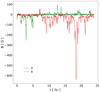 |
Fig. 3. Magnetic field strength time variation, B(t), for the two pixels marked in the right panel of Fig. 1. Specifically, the green line corresponds to pixel A, while the red one to pixel B. The black horizontal line at B = 0 is for reference. |
3.2. The Hölder-Hurst exponent in the quiet Sun
Now that the stationarity of B(t) within the FoV (Sect. 3.1) has been established, we can apply the techniques described in Sect. 2.2 that are designed to reveal the persistent or antipersistent nature of fluctuations in the quiet Sun. The statistical properties of magnetic field fluctuations in a complex environment affected by turbulent convection, such as the photosphere of the quiet Sun, can be studied through the classical approach of scaling analysis of structure functions (see, e.g. Frisch 1995). Structure functions have the ability to capture the scaling features of stationary signals and reveal their characteristics, such as the turbulent nature of fluctuations. The set of scaling exponents, ξ(q), allows us to infer quantities such as the degree of intermittency and identifying the model that best reproduces the observed scaling properties (Frisch 1995). For example, if the model best describing the observed fluctuations is a classical Kolmogorov’s homogeneous and isotropic turbulence, we observe the scaling exponents ξ(1)=1/3 and ξ(q)=q/3 in the inertial range. Conversely, in the presence of more complex dynamics, a non-linear dependence of ξ(q) on q is revealed, and anomalous scaling emerges. Thus, in our case, structure functions are capable of characterising the properties of B(t) fluctuations in the FoV; they can be defined, in an equivalent way, as the moments of order q of the probability density functions (PDFs) of B(t) fluctuations at scale τ (see Eq. (1)). The structure function of order q = 1, namely S1(τ), was computed in the FoV by following Eq. (1). In Fig. 4, we show S1 for τ = 90 s, which is the shortest timescale accessible. S1(τ = 90 s) ranges between ≃4.2 G and ≃26.0 G and is saturated between 4 G and 14 G. The boundary of the supergranular cell is clearly enhanced, meaning that the amplitude of magnetic field fluctuations at the scale τ is appreciably higher in the boundaries than in the inner part of the supergranule. This is also directly visible in Fig. 3 concerning the comparison between the magnetic field strength signals in the two environments, A and B, marked with arrows in Fig. 1. The scaling exponent ξ(1) in the FoV can be computed in those ranges of τ where scale invariance holds, that is, where Eq. (2) is satisfied. This condition corresponds to a linear behaviour of S1 with τ in a log-log plot. Figure 5 shows S1 as a function of τ in a log-log plot for the points A and B of the FoV. Standard errors associated with the values of the structure function at any τ are smaller than the symbols used in the plot. A linear behaviour is well visible at least up to τ ≃ 103 s, indicating a self-similar and scale-invariant behaviour up to that timescale. The slopes of the linear trends correspond to the scaling exponents for both environments, A and B. For each pixel of the FoV, we computed log(S1) versus log τ and fitted with a line with a slope ξ(1). The condition that the interval in τ covers at least a decade is imposed in order to guarantee a sufficient statistical robustness in finding the scaling exponents. The slope of the best-fitting line obtained corresponds to the Hölder-Hurst exponent, H. This procedure allowed us to retrieve the map of the Hölder-Hurst exponent in the FoV shown in Fig. 6. H ranges between ≃0.1 and ≃0.7, with the highest values in correspondence of the boundary of the supergranule, where the network magnetic fields take place, while the lower values are observed both inside and outside the supergranule, that is, reasonably inside supergranules adjacent to that represented in the FoV (Gošić et al. 2014).
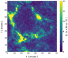 |
Fig. 4. Structure functions S1 for τ = 90 s in the whole FoV, saturated between 4 and 14 G. |
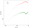 |
Fig. 5. Log–log plot of structure function of order 1 as a function of the timescale τ for the pixels A and B identified in the right panel of Fig. 1. Green stars mark S1, A, while red dots mark S1, B. Standard errors associated with the values of the structure function at any τ are smaller than the symbols used, and are therefore not visible in this representation. |
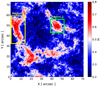 |
Fig. 6. Map of Hölder-Hurst exponent in the FoV saturated between 0.3 and 0.7. The yellow and green boxes identify Region 1 and Region 2, respectively (see the text). |
4. Discussion
In a series of papers beginning in 2013, Giannattasio and collaborators studied the motion tracks and dynamic properties of magnetic elements (MEs) in the same quiet Sun region. They investigated both the mean square displacement and the time-varying probability density function of displacements under the hypothesis that photospheric MEs are passively transported by the underlying plasma flow (Giannattasio et al. 2013, 2014a,b; Giannattasio et al. 2019; Caroli et al. 2015; Giannattasio & Consolini 2021). This revealed properties of the plasma velocity field, which is driven by turbulent convection. In the present study, we investigated the scaling properties of magnetic field fluctuations instead of the velocity field properties in the quiet Sun by analysing a long (∼24 h) time-series of magnetograms targeted at a photospheric region that encloses a whole supergranule. This allowed us to characterise magnetic field fluctuations in an environment representative of the quiet Sun. This task was accomplished by analysing first-order structure functions and the map of H values in the FoV, which link the character of magnetic fluctuations to the local environment probed. This map provided a unique opportunity to identify different features of magnetic field fluctuations originated by different physical processes. This has been possible without any model describing the physical characteristics and dynamic properties of the magnetic fields in the quiet Sun, studying only their time correlation on supergranular spatial and temporal scales. Indeed, large values of H are associated with features that must hold a large spatiotemporal coherence with respect to features characterised by smaller values of H.
A general feature emerging from our analysis is that the character of magnetic field fluctuations crucially depends on the environment inside the FoV, whereby they are persistent (H > 0.5) in the boundary of the supergranule and antipersistent (H < 0.5) inside it. Giannattasio et al. (2018) evaluated the magnetic field decorrelation times in the same FoV, namely tD, defined as the times at which the magnetic field autocorrelation function decreases by a factor 1/e and showed a map of these values in the same FoV. Values were found to range between 30 and 240 min in the supergranular boundary, and between 30 and 50 min inside the supergranule. In particular, the highest values of tD are found in the region between X = 0 arcsec and X = 10 arcsec, and Y = 30 arcsec and Y = 60 arcsec (Region 1 in Fig. 6), in coincidence with H > 0.5. Conversely, low values of tD characterise the regions between X = 40 arcsec and X = 50 arcsec, and Y = 45 arcsec and Y = 55 arcsec (Region 2 in Fig. 6), in coincidence with the highest values of H. Inside the supergranule, both H and tD values are small. This suggests that in environments such as Region 1, magnetic field fluctuations coherently and slowly decrease or increase such to keep long tD. On the other hand, in environments such as Region 2, magnetic field fluctuations are even more persistent than in Region 1 (the values of H reach a maximum in the FoV, namely Hmax ∼ 0.7), despite the low values of tD. This behaviour can be explained by considering that Region 2 hosts a stable vortex-like plasma flow, as reported by Requerey et al. (2018), Chian et al. (2019) and Giannattasio et al. (2020). The intense downflow associated with the vortex may behave like an attractor, constraining the motion of MEs in such a relatively small region. The packing of different MEs moving quickly due to the vortex may result, in those pixels, in reduced values of tD and, at the same time, increasing magnetic field fluctuations, giving rise to high values of H. Finally, within the supergranule, magnetic field fluctuations are antipersistent (H < 0.5) and quickly decorrelate the pixel-by-pixel magnetic field. Coherent magnetic features are certainly present in the form of MEs, but they rapidly evolve, being dragged along the horizontal velocity field, and do not stay at the same location for a sufficiently long time to locally maintain a time-correlated magnetic field (see, e.g. Giannattasio et al. 2013). Thus, the Hölder-Hurst exponent complements the information provided by tD, pointing out that processes generating very different decorrelation times (like those found in Regions 1 and 2) may also affect magnetic field fluctuations in a similar way and, in principle, they can be ascribed to similar processes in both sites. According to this interpretation, while it is possible to consistently explain the cases of (i) high H and long tD, (ii) high H and short tD, and (iii) low H and short tD, it is difficult to justify the simultaneous occurrence of low H and long tD values in the same location, a condition that never occurs in the FoV. This confirms the significant role of H in characterising the dynamic properties of magnetic fields in the quiet Sun.
We also notice that high values of H coincide with high values of occurrence, as shown in Fig. 3 of Giannattasio et al. (2018). In that work, occurrence is defined as the percentage of observational time in which a pixel in the FoV is filled with magnetic field. Here, the maximum occurrence is located in Region 2 of Fig. 6, where it reaches ≃100% and where the maximum H also occurs. In this region, again, the relatively short tD indicates a fast renewal of the magnetic field content with fluctuations clustered in one direction, suggesting that the site is one of long-term increasing fluctuation fields on supergranular timescales. This behaviour is not immediately detectable by looking only at changes in magnetic field strength over time (see the example of the red track in Fig. 3; Pixel B is, in fact, within Region 2). A possible scenario is the presence of different packed MEs occupying a small region, which agrees with the low (horizontal) diffusion of small-scale magnetic fields and their quasi-random trajectories (Giannattasio et al. 2013, 2014a), which is probably due to intense downflows behaving like attractors for MEs. This is consistent with the presence of strong and persistent downflows in all regions characterised by high values of both H and degree of occurrence, as is evident in Fig. 2, which represents the mean plasma vertical velocity detected in the FoV. In that figure, downflows on the boundary of the supergranular cell behave like long-correlated features co-spatial with the loci where magnetic fields in the quiet Sun pile up, exhibiting clustered fluctuations with a high degree of persistency. The presence of an intense downflow associated with the peak of H in Region 2 is also corroborated by the presence, as mentioned above, of a vortex, similarly to what is detected in other works (see, e.g. Bonet et al. 2008, 2010), and predicted by simulations (see, e.g. Shelyag et al. 2011). The presence of vortexes is consistent with the fast variation of magnetic field.
The map of H displayed in Fig. 6 can also be compared with the map of time-averaged magnetic energy variations in the same FoV reported in Fig. 4 by Giannattasio et al. (2020). In that work, the authors applied Poynting’s theorem to investigate the magnetic energy balance of the quiet photosphere on supergranular timescales, ⟨Δu⟩, and found that the timescale, associated with the energy variation of a plasma volume element, τ*, is of the same order of magnitude as tD. In particular, the maximum value of tD is located in the region identified as Region 1 in Fig. 6 and, more in general, where ⟨Δu⟩≥0, that is, where the energy content is stationary or slightly positive in contrast with the field decay (and following decorrelation). The only exception is, again, the region identified as Region 2 in Fig. 6, where ⟨Δu⟩≃0 and tD is relatively short. In this case, the presence of an intense vortex flow, which has been reported in the literature to constrain the dynamics of tightly packed MEs, well explains this feature. The key point is that the energy variation averaged on supergranular scales, ⟨Δu⟩≥0, is consistent with the H map, which is expected, because a statistical and long-correlated increase in magnetic field fluctuations should translate into an increase in the available magnetic energy.
Further insight can be obtained by discussing the map of H in the context of the different turbulent regimes that small-scale magnetic fields in the quiet Sun may follow. For stationary and scale-invariant signals, the power spectral density of fluctuations, S(f), is expected to scale as
 (8)
(8)
where f = τ−1 is the frequency and β the scaling exponent. Under this hypothesis, a relation occurs between H and β, namely
 (9)
(9)
This, of course, implies that different values of H correspond bijectively to different values of β, and maps of H or β provide the same information. Thus, knowledge of H also reveals the energy spectral content of fluctuations and, accordingly, the dynamic properties of the quiet Sun. We note that Eq. (9) holds only in the case where corrections due to intermittency are absent; otherwise this relation should be replaced with β < 2H + 1. Due to Eq. (9), the spectral index lies within the range β ∈ [1, 3]. In particular, antipersistent fluctuations correspond to β ∈ [1, 2), while persistent fluctuations correspond to β ∈ (2, 3]. The different characters of spectral features in the FoV may be the consequence of the different turbulent regimes followed by convection. This agrees with the findings of previous studies, where different dynamic regimes in the FoV were identified using different techniques (see, e.g. Giannattasio et al. 2014a,b, 2018). For example, the value H = 0.33, which corresponds to β = 1.66, is the value expected according the Kolmogorov’s K41 theory for fluid, homogeneous and isotropic turbulent environments in the absence of intermittency effects (Frisch 1995). As we can see in Fig. 6, this dynamic regime is observed in the inner regions of the supergranule. Due to the intermittency effect, there may be some slight variations in the β spectral exponent value expected in the case of K41 theory. Consequently, because of the intermittent effect, the H values may also be subjected to slight variations around the 0.33 value (see, e.g. Ruiz-Chavarria et al. 1996). In the FoV examined in this work, values of H between 0.3 and 0.4 are mainly found in the central regions of the supergranule. Inside the supergranule, different scenarios matching antipersistency are possible: (1) the processes occurring therein and giving rise to the observed magnetic field fluctuations are consistent with turbulent convection obeying the Kolmogorov’s legacy with H = 0.33 and ξ(2)=0.66; (2) we are in the presence of a regime characterised by a strong intermittency (e.g. due to the behaviour of MEs being comparable to that of passive scalars) for which ξ(2)≠2H; (3) we are in the presence of quasi-Brownian processes with ξ(2)∼1 and H ∼ 0.5; or (4) we are in the presence of other regimes characterised by different scaling laws and H and ξ(2) values. At this time, it is not possible to precisely discriminate between those different regimes, as longer time-series are necessary to study the higher orders of the structure functions (Frisch 1995).
In conclusion, the scaling properties of magnetic field in the quiet Sun may help to characterise its evolution driven by turbulent convection and can offer a perspective that is different from that provided by other techniques, such as those applied in previous works inherent to the same FoV. This approach confers an advantage in that it does not require assumptions as to the passivity of MEs. In fact, in this work, we did not use any transport phenomena as diagnostic of the dynamic properties of the quiet Sun.
5. Summary and conclusions
Some aspects inherent to the physics of the quiet Sun remain poorly understood. One of these deals with the physical processes capable of storing energy in the photosphere, making it available for the upper atmospheric layers, where it is eventually dissipated and contributes to local heating. In this framework, approaching the quiet Sun as a complex system may provide dynamic constraints for future models aiming to explain both the origin and variation of the magnetic energy content in the quiet Sun from (sub)granular to (at least) supergranular spatial and temporal scales. The analysis proposed in this work characterises the magnetic field fluctuations, pointing out their link with the local environment. In particular, we take advantage of a diagnostic that exploits the structure function analysis typically used in the field of turbulence, for example. This diagnostic, namely the Hölder-Hurst exponent, is able to detect the persistent or antipersistent character of fluctuations and may help to distinguish between different dynamic regimes in action, which are responsible for the observed magnetic field fluctuations. The physical framework that seems to emerge from our analysis tells us that magnetic patterns and convective structures determine different local dynamic regimes in the solar plasma that lead to different behaviours in the dynamic properties of MEs.
The results obtained in this work can be briefly itemised as follows:
-
We computed first-order structure functions associated with the magnetic field fluctuations in the FoV. Under the verified hypothesis of stationarity, such structure functions scale like a power law.
-
The scaling indices of the power law, which depend on the considered order, were used to compute, for the first time, the Hölder-Hurst exponent in the FoV.
-
We find that magnetic field fluctuations are mainly persistent at the boundary of the supergranule, where intense and persistent downflows are observed, and anti-persistent inside it. This suggests that different environments in the FoV undergo different dynamic regimes. We interpret our results in the context of the current literature.
In conclusion, our findings suggest that the persistence in sign of magnetic field fluctuations as measured by H reveal the existence of different dynamic regimes in action in the quiet Sun capable of generating the observed magnetic field fluctuations, such as three dimensional or two dimensional reduced magnetohydrodynamic turbulence. The robustness of our results is corroborated by their consistency with the previous literature, despite the great diversity of the techniques applied. In the future, it will be important to investigate the scaling properties of other physical quantities playing a fundamental role in the quiet Sun, such as velocity (both horizontal and vertical), vorticity, and electric and current density fields, to mention just a few. This will greatly improve our knowledge of the physical processes responsible for the storage and evolution of the great amount of energy available in the quiet Sun. This energy may be transported to the upper atmospheric layers, dissipated therein, and eventually start a chain of phenomena relevant to space weather.
Acknowledgments
We thank the referee, Prof. V.I. Abramenko, for her report and insightful comments on our work. This work is supported by Italian MIUR-PRIN grant 2017APKP7T on Circumterrestrial Environment: Impact of Sun-Earth Interaction. F.G. is grateful to L. Bellot Rubio and M. Gošić for having provided the data set used in this work. This paper is based on data acquired in the framework of the Hinode Operation Plan 151 entitled “Flux replacement in the network and internetwork”. Hinode is a Japanese mission developed and launched by ISAS/JAXA, collaborating with NAOJ as a domestic partner, NASA and STFC (UK) as international partners. Scientific operation of the Hinode mission is conducted by the Hinode science team organized at ISAS/JAXA. This team mainly consists of scientists from institutes in the partner countries. Support for the post-launch operation is provided by JAXA and NAOJ (Japan), STFC (UK), NASA, ESA, and NSC (Norway).
References
- Abramenko, V. I. 2014, Geomagn. Aeron., 54, 892 [CrossRef] [Google Scholar]
- Abramenko, V. I. 2017, MNRAS, 471, 3871 [NASA ADS] [CrossRef] [Google Scholar]
- Abramenko, V. I., Yurchyshyn, V. B., Wang, H., Spirock, T. J., & Goode, P. R. 2002, ApJ, 577, 487 [NASA ADS] [CrossRef] [Google Scholar]
- Abramenko, V. I., Carbone, V., Yurchyshyn, V., et al. 2011, ApJ, 743, 133 [NASA ADS] [CrossRef] [Google Scholar]
- Agrawal, P., Rast, M. P., Gošić, M., Bellot Rubio, L. R., & Rempel, M. 2018, ApJ, 854, 118 [NASA ADS] [CrossRef] [Google Scholar]
- Akaike, H. 1974, IEEE Trans. Autom. Control, 19, 716 [Google Scholar]
- Beeck, B., Collet, R., Steffen, M., et al. 2012, A&A, 539, A121 [NASA ADS] [CrossRef] [EDP Sciences] [Google Scholar]
- Bellot Rubio, L., & Orozco Suárez, D. 2019, Liv. Rev. Sol. Phys., 16, 1 [Google Scholar]
- Berger, T. E., Löfdahl, M. G., Shine, R. A., & Title, A. M. 1998, ApJ, 506, 439 [NASA ADS] [CrossRef] [Google Scholar]
- Berrilli, F., Florio, A., Consolini, G., et al. 1999, A&A, 344, L29 [NASA ADS] [Google Scholar]
- Berrilli, F., Consolini, G., Pietropaolo, E., et al. 2002, A&A, 381, 253 [NASA ADS] [CrossRef] [EDP Sciences] [Google Scholar]
- Berrilli, F., Del Moro, D., Consolini, G., et al. 2004, Sol. Phys., 221, 33 [NASA ADS] [CrossRef] [Google Scholar]
- Berrilli, F., del Moro, D., Florio, A., & Santillo, L. 2005, Sol. Phys., 228, 81 [CrossRef] [Google Scholar]
- Berrilli, F., Scardigli, S., & Giordano, S. 2013, Sol. Phys., 282, 379 [NASA ADS] [CrossRef] [Google Scholar]
- Berrilli, F., Scardigli, S., & Del Moro, D. 2014, A&A, 568, A102 [NASA ADS] [CrossRef] [EDP Sciences] [Google Scholar]
- Bonet, J. A., Márquez, I., Sánchez Almeida, J., Cabello, I., & Domingo, V. 2008, ApJ, 687, L131 [Google Scholar]
- Bonet, J. A., Márquez, I., Sánchez Almeida, J., et al. 2010, ApJ, 723, L139 [Google Scholar]
- Brandt, P. N., & Getling, A. V. 2008, Sol. Phys., 249, 307 [CrossRef] [Google Scholar]
- Burnham, K., & Anderson, D. 2002, Model Selection and Multimodel Inference: A Practical Information-Theoretic Approach (New York: Springer-Verlag) [Google Scholar]
- Cadavid, A. C., Lawrence, J. K., Ruzmaikin, A. A., Walton, S. R., & Tarbell, T. 1998, ApJ, 509, 918 [NASA ADS] [CrossRef] [Google Scholar]
- Cadavid, A. C., Lawrence, J. K., & Ruzmaikin, A. A. 1999, ApJ, 521, 844 [CrossRef] [Google Scholar]
- Caroli, A., Giannattasio, F., Fanfoni, M., et al. 2015, J. Plasma Phys., 81, 495810514 [NASA ADS] [CrossRef] [Google Scholar]
- Cattaneo, F., Emonet, T., & Weiss, N. 2003, ApJ, 588, 1183 [NASA ADS] [CrossRef] [Google Scholar]
- Centeno, R., Socas-Navarro, H., Lites, B., et al. 2007, ApJ, 666, L137 [CrossRef] [Google Scholar]
- Chae, J., & Sakurai, T. 2008, ApJ, 689, 593 [NASA ADS] [CrossRef] [Google Scholar]
- Chian, A. C.-L., Silva, S. S. A., Rempel, E. L., et al. 2019, MNRAS, 488, 3076 [Google Scholar]
- Consolini, G., Carbone, V., Berrilli, F., et al. 1999, A&A, 344, L33 [NASA ADS] [Google Scholar]
- Danilovic, S., Cameron, R. H., & Solanki, S. K. 2015, A&A, 574, A28 [NASA ADS] [CrossRef] [EDP Sciences] [Google Scholar]
- De Pontieu, B., McIntosh, S. W., Carlsson, M., et al. 2007, Science, 318, 1574 [Google Scholar]
- de Wijn, A. G., Lites, B. W., Berger, T. E., et al. 2008, ApJ, 684, 1469 [NASA ADS] [CrossRef] [Google Scholar]
- Del Moro, D. 2004, A&A, 428, 1007 [NASA ADS] [CrossRef] [EDP Sciences] [Google Scholar]
- Del Moro, D., Berrilli, F., Duvall, T. L., & Kosovichev, A. G. 2004, Sol. Phys., 221, 23 [CrossRef] [Google Scholar]
- Del Moro, D., Giannattasio, F., Berrilli, F., et al. 2015, A&A, 576, A47 [NASA ADS] [CrossRef] [EDP Sciences] [Google Scholar]
- Elliott, G., Rothenberg, T. J., & Stock, J. H. 1996, Econometrica, 64, 813 [CrossRef] [Google Scholar]
- Frisch, U. 1995, Turbulence. The Legacy of A. N. Kolmogorov (Cambridge: Cambridge University Press), 296 [Google Scholar]
- Fuller, W. A. 1977, J. R. Stat. Soc. Ser. A, 140, 277 [CrossRef] [Google Scholar]
- Getling, A. V. 2006, Sol. Phys., 239, 93 [CrossRef] [Google Scholar]
- Getling, A. V., & Brandt, P. N. 2002, A&A, 382, L5 [NASA ADS] [CrossRef] [EDP Sciences] [Google Scholar]
- Giannattasio, F., & Consolini, G. 2021, ApJ, 908, 142 [NASA ADS] [CrossRef] [Google Scholar]
- Giannattasio, F., Del Moro, D., Berrilli, F., et al. 2013, ApJ, 770, L36 [NASA ADS] [CrossRef] [Google Scholar]
- Giannattasio, F., Stangalini, M., Berrilli, F., Del Moro, D., & Bellot Rubio, L. 2014a, ApJ, 788, 137 [NASA ADS] [CrossRef] [Google Scholar]
- Giannattasio, F., Berrilli, F., Biferale, L., et al. 2014b, A&A, 569, A121 [NASA ADS] [CrossRef] [EDP Sciences] [Google Scholar]
- Giannattasio, F., Berrilli, F., Consolini, G., et al. 2018, A&A, 611, A56 [NASA ADS] [CrossRef] [EDP Sciences] [Google Scholar]
- Giannattasio, F., Consolini, G., Berrilli, F., & Del Moro, D. 2019, ApJ, 878, 33 [NASA ADS] [CrossRef] [Google Scholar]
- Giannattasio, F., Consolini, G., Berrilli, F., & Del Moro, D. 2020, ApJ, 904, 7 [NASA ADS] [CrossRef] [Google Scholar]
- Gošić, M., Bellot Rubio, L. R., Orozco Suárez, D., Katsukawa, Y., & del Toro Iniesta, J. C. 2014, ApJ, 797, 49 [Google Scholar]
- Gošić, M., Bellot Rubio, L. R., del Toro Iniesta, J. C., Orozco Suárez, D., & Katsukawa, Y. 2016, ApJ, 820, 35 [Google Scholar]
- Gošić, M., de la Cruz Rodríguez, J., De Pontieu, B., et al. 2018, ApJ, 857, 48 [CrossRef] [Google Scholar]
- Guevara Gómez, J. C., Jafarzadeh, S., Wedemeyer, S., et al. 2021, Phil. Trans. R. Soc. London Ser. A, 379, 20200184 [Google Scholar]
- Hagenaar, H. J., Schrijver, C. J., Title, A. M., & Shine, R. A. 1999, ApJ, 511, 932 [CrossRef] [Google Scholar]
- Hurst, H.E. 1956, Proc. Inst. Civ. Eng., 5, 519 [Google Scholar]
- Jefferies, S. M., McIntosh, S. W., Armstrong, J. D., et al. 2006, ApJ, 648, L151 [Google Scholar]
- Jess, D. B., Keys, P. H., Stangalini, M., & Jafarzadeh, S. 2021, Phil. Trans. R. Soc. London Ser. A, 379, 20200169 [Google Scholar]
- Keys, P. H., Mathioudakis, M., Jess, D. B., Mackay, D. H., & Keenan, F. P. 2014, A&A, 566, A99 [NASA ADS] [CrossRef] [EDP Sciences] [Google Scholar]
- Keys, P. H., Reid, A., Mathioudakis, M., et al. 2019, MNRAS, 488, L53 [NASA ADS] [Google Scholar]
- Keys, P. H., Reid, A., Mathioudakis, M., et al. 2020, A&A, 633, A60 [NASA ADS] [CrossRef] [EDP Sciences] [Google Scholar]
- Khomenko, E., Vitas, N., Collados, M., & de Vicente, A. 2017, A&A, 604, A66 [NASA ADS] [CrossRef] [EDP Sciences] [Google Scholar]
- Kosugi, T., Matsuzaki, K., Sakao, T., et al. 2007, Sol. Phys., 243, 3 [Google Scholar]
- Kutsenko, A. S., Abramenko, V. I., Kuzanyan, K. M., Xu, H., & Zhang, H. 2018, MNRAS, 480, 3780 [NASA ADS] [CrossRef] [Google Scholar]
- Lawrence, J. K., Cadavid, A. C., & Ruzmaikin, A. A. 1994, Sol. Surf. Magn., 433, 279 [CrossRef] [Google Scholar]
- Lawrence, J. K., Cadavid, A. C., Ruzmaikin, A., & Berger, T. E. 2001, Phys. Rev. Lett., 86, 5894 [NASA ADS] [CrossRef] [Google Scholar]
- Lepreti, F., Carbone, V., Abramenko, V. I., et al. 2012, ApJ, 759, L17 [NASA ADS] [CrossRef] [Google Scholar]
- MacKinnon, J. G. 1994, J. Bus. Econ. Stat., 12, 167 [Google Scholar]
- Manso Sainz, R., Martínez González, M. J., & Asensio Ramos, A. 2011, A&A, 531, L9 [NASA ADS] [CrossRef] [EDP Sciences] [Google Scholar]
- Nesis, A., Hammer, R., Roth, M., & Schleicher, H. 2006, A&A, 451, 1081 [NASA ADS] [CrossRef] [EDP Sciences] [Google Scholar]
- November, L. J. 1980, Ph.D. Thesis, Colorado Univ., USA. [Google Scholar]
- Orozco Suárez, D., Katsukawa, Y., & Bellot Rubio, L. R. 2012, ApJ, 758, L38 [CrossRef] [Google Scholar]
- Rajaguru, S. P., Sangeetha, C. R., & Tripathi, D. 2019, ApJ, 871, 155 [Google Scholar]
- Rast, M. P. 2002, A&A, 392, L13 [NASA ADS] [CrossRef] [EDP Sciences] [Google Scholar]
- Rempel, M. 2014, ApJ, 789, 132 [Google Scholar]
- Rempel, M., Schüssler, M., Cameron, R. H., & Knölker, M. 2009, Science, 325, 171 [CrossRef] [Google Scholar]
- Requerey, I. S., Cobo, B. R., Gošić, M., & Bellot Rubio, L. R. 2018, A&A, 610, A84 [NASA ADS] [CrossRef] [EDP Sciences] [Google Scholar]
- Roudier, T., Malherbe, J. M., Vigneau, J., & Pfeiffer, B. 1998, A&A, 330, 1136 [NASA ADS] [Google Scholar]
- Roudier, T., Malherbe, J. M., Rieutord, M., & Frank, Z. 2016, A&A, 590, A121 [NASA ADS] [CrossRef] [EDP Sciences] [Google Scholar]
- Rouppe van der Voort, L. H. M., Rutten, R. J., & Vissers, G. J. M. 2016, A&A, 592, A100 [NASA ADS] [CrossRef] [EDP Sciences] [Google Scholar]
- Ruiz-Chavarria, G., Baudet, C., & Ciliberto, S. 1996, Phys. D: Nonlinear Phenom., 99, 369 [NASA ADS] [CrossRef] [Google Scholar]
- Said, S. E., & Dickey, D. A. 1984, Biometrika, 71, 599 [CrossRef] [Google Scholar]
- Sánchez Almeida, J., Bonet, J. A., Viticchié, B., & Del Moro, D. 2010, ApJ, 715, L26 [CrossRef] [Google Scholar]
- Shelyag, S., Keys, P., Mathioudakis, M., & Keenan, F. P. 2011, A&A, 526, A5 [NASA ADS] [CrossRef] [EDP Sciences] [Google Scholar]
- Stangalini, M. 2014, A&A, 561, L6 [NASA ADS] [CrossRef] [EDP Sciences] [Google Scholar]
- Stangalini, M., Consolini, G., Berrilli, F., De Michelis, P., & Tozzi, R. 2014, A&A, 569, A102 [NASA ADS] [CrossRef] [EDP Sciences] [Google Scholar]
- Stangalini, M., Giannattasio, F., & Jafarzadeh, S. 2015, A&A, 577, A17 [NASA ADS] [CrossRef] [EDP Sciences] [Google Scholar]
- Stangalini, M., Giannattasio, F., Erdélyi, R., et al. 2017, ApJ, 840, 19 [NASA ADS] [CrossRef] [Google Scholar]
- Stein, R. F., & Nordlund, Å. 1998, ApJ, 499, 914 [Google Scholar]
- Stein, R. F., & Nordlund, Å. 2001, ApJ, 546, 585 [Google Scholar]
- Stenflo, J. O. 2012, A&A, 541, A17 [NASA ADS] [CrossRef] [EDP Sciences] [Google Scholar]
- Tomczyk, S., McIntosh, S. W., Keil, S. L., et al. 2007, Science, 317, 1192 [Google Scholar]
- Tsuneta, S., Ichimoto, K., Katsukawa, Y., et al. 2008, Sol. Phys., 249, 167 [Google Scholar]
- Viticchié, B., Del Moro, D., & Berrilli, F. 2006, ApJ, 652, 1734 [CrossRef] [Google Scholar]
- Vögler, A., Shelyag, S., Schüssler, M., et al. 2005, A&A, 429, 335 [Google Scholar]
- Wang, H. 1988, Sol. Phys., 116, 1 [CrossRef] [Google Scholar]
- Yang, Y., Ji, K., Feng, S., et al. 2015a, ApJ, 810, 88 [NASA ADS] [CrossRef] [Google Scholar]
- Yang, Y.-F., Qu, H.-X., Ji, K.-F., et al. 2015b, Res. Astron. Astrophys., 15, 569 [CrossRef] [Google Scholar]
- Yelles Chaouche, L., Moreno-Insertis, F., Martínez Pillet, V., et al. 2011, ApJ, 727, L30 [NASA ADS] [CrossRef] [Google Scholar]
All Figures
|
Fig. 1. Left panel: first frame of the magnetogram time-series acquired on 2010 November 2 at 08:00:42 UT, saturated between −600 G and 600 G; Right panel: mean magnetogram averaged over the entire magnetogram time-series (∼24 h) saturated between −300 G and 300 G. The green and red arrows point to two pixels belonging to inner (A) and boundary (B) regions of the supergranule, respectively. |
| In the text | |
|
Fig. 2. Mean plasma vertical velocity over the entire dopplergram time-series saturated between −0.1 km s−1 and 0.1 km s−1. Positive (red) velocities indicate redshifted downflowing plasma, while negative (blue) velocities indicate blueshifted upflowing plasma. |
| In the text | |
|
Fig. 3. Magnetic field strength time variation, B(t), for the two pixels marked in the right panel of Fig. 1. Specifically, the green line corresponds to pixel A, while the red one to pixel B. The black horizontal line at B = 0 is for reference. |
| In the text | |
|
Fig. 4. Structure functions S1 for τ = 90 s in the whole FoV, saturated between 4 and 14 G. |
| In the text | |
|
Fig. 5. Log–log plot of structure function of order 1 as a function of the timescale τ for the pixels A and B identified in the right panel of Fig. 1. Green stars mark S1, A, while red dots mark S1, B. Standard errors associated with the values of the structure function at any τ are smaller than the symbols used, and are therefore not visible in this representation. |
| In the text | |
|
Fig. 6. Map of Hölder-Hurst exponent in the FoV saturated between 0.3 and 0.7. The yellow and green boxes identify Region 1 and Region 2, respectively (see the text). |
| In the text | |
Current usage metrics show cumulative count of Article Views (full-text article views including HTML views, PDF and ePub downloads, according to the available data) and Abstracts Views on Vision4Press platform.
Data correspond to usage on the plateform after 2015. The current usage metrics is available 48-96 hours after online publication and is updated daily on week days.
Initial download of the metrics may take a while.