| Issue |
A&A
Volume 659, March 2022
|
|
|---|---|---|
| Article Number | A42 | |
| Number of page(s) | 18 | |
| Section | Planets and planetary systems | |
| DOI | https://doi.org/10.1051/0004-6361/202142571 | |
| Published online | 04 March 2022 | |
Dust entrainment in magnetically and thermally driven disk winds
Institute for Theoretical Astrophysics, Zentrum für Astronomie, Heidelberg University,
Albert-Ueberle-Str. 2,
69120
Heidelberg,
Germany
e-mail: This email address is being protected from spambots. You need JavaScript enabled to view it.
Received:
2
November
2021
Accepted:
24
December
2021
Abstract
Context. Magnetically and thermally driven disk winds have gained popularity in the light of the current paradigm of low viscosities in protoplanetary disks that nevertheless present large accretion rates even in the presence of inner cavities. The possibility of dust entrainment in these winds may explain recent scattered light observations and constitutes a way of dust transport towards outer regions of the disk.
Aims. We aim to study the dust dynamics in these winds and explore the differences between photoevaporation and magnetically driven disk winds in this regard. We quantify maximum entrainable grain sizes, the flow angle, and the general detectability of such dusty winds.
Methods. We used the FARGO3D code to perform global, 2.5D axisymmetric, nonideal MHD simulations including ohmic and ambipolar diffusion. Dust was treated as a pressureless fluid. Synthetic observations were created with the radiative transfer code RADMC-3D.
Results. We find a significant difference in the dust entrainment efficiency of warm, ionized winds such as photoevaporation and magnetic winds including X-ray and extreme ultraviolet heating compared to cold magnetic winds. The maximum entrainable grain size varies from 3 μm−6 μm for ionized winds to 1 μm for cold magnetic winds. The dust flow angle decreases rapidly with increasing grain size. Dust grains in cold magnetic winds tend to flow along a shallower angle compared to the warm, ionized winds. With increasing distance to the central star, the dust entrainment efficiency decreases. Larger values of the turbulent viscosity increase the maximum grain size radius of possible dust entrainment. Our simulations indicate that diminishing dust content in the outer regions of the wind can be mainly attributed to the dust settling in the disk. The Stokes number along the wind launching front stays constant in the outer region. In the synthetic images, the dusty wind appears as a faint, conical emission region which is brighter for a cold magnetic wind.
Key words: protoplanetary disks / hydrodynamics / radiative transfer / magnetic fields / magnetohydrodynamics (MHD) / ISM: jets and outflows
© ESO 2022
1 Introduction
The limited lifetime of a few million years (Haisch et al. 2001; Mamajek et al. 2004; Ribas et al. 2015) of protoplanetary disks has sparked interest in various mechanisms that transport and extract angular momentum from the disk. One possibility to drive accretion onto the central star is viscous turbulence, usually referred to as α-viscosity in the context of disks (Shakura & Sunyaev 1973). Turbulence might be generated by a multitude of physical instabilities in gas and dust. The well studied magnetorotational instability (MRI; Balbus & Hawley 1991) present in an ionized, differentially rotating disk threaded by a weak magnetic field can lead to values of α roughly ranging from 10−3 to 10−2 and it was studied in a local shearing box (Fromang & Papaloizou 2007; Fromang et al. 2007; Bai 2011) as well as in global simulations (Dzyurkevich et al. 2010; Flock et al. 2011).
The MRI can only operate if the ionization fraction of gas is sufficiently high, which is not necessarily the case in the midplane of the disk (Igea & Glassgold 1999), where nonideal magnetohydrodynamic (MHD) effects such as ohmic diffusion dominate. These so-called dead zones prevent magnetically driven accretion in the midplane, whereas layered accretion in the ionized upper part of the disk atmosphere is still possible (Gammie 1996). In the more dilute outer regions of the disk, the ionization fraction rises again and the edge between the inner dead zone and the outer MRI-active part might cause jumps in the density profile and therewith enable dust or pebble traps (Lyra et al. 2009; Dzyurkevich et al. 2010, 2013). Purely hydrodynamic instabilities such as the global baroclinic instability (Klahr & Bodenheimer 2003) and the convective overstability (Klahr & Hubbard 2014), on the other hand, are alternative turbulence driving mechanisms that can also operate in the weakly ionized parts of the disk. In the presence of short gas cooling times, the vertical shear instability (VSI) causes vertical oscillations which are able to transport small dust grains towards the upper layers of the disk (Stoll & Kley 2014, 2016; Flock et al. 2020; Blanco et al. 2021). Vortices triggered by the VSI in combination with the Rossby wave instability (Lovelace et al. 1999) may act as long-lived dust traps (Manger & Klahr 2018; Pfeil & Klahr 2021).
Since recent observation hint towards small viscosity and thus small values of α on the order of 10−4 to 10−3 (Flaherty et al. 2015, 2017), the effect of disk winds might be a possible explanation for the finite disk lifetimes. In the context of photoevaporation, ionizing radiation either from the central star or the from the stellar environment heats the surface layers of the disk and drives winds due to the thermal pressure gradient. Depending on the dominant type of radiation, the wind mass loss rates are on the order of 10−10 M⊙ yr−1 with EUV radiation (Hollenbach et al. 1994; Font et al. 2004), and 10−8 M⊙ yr−1 to 10−7 M⊙ yr−1 with FUV radiation (Adams et al. 2004; Gorti & Hollenbach 2009) and X-ray radiation (Ercolano et al. 2009, 2021; Owen et al. 2010, 2012; Picogna et al. 2019, 2021).
An alternative way to produce strong disk winds would be by considering the effect of magnetic fields. In the presence of a global magnetic field the differential shearing motion of the disk generates a magnetic pressure gradient, accelerating matter and thereby driving the outflow. In the strong field limit, the gas follows the magnetic field lines and is magneto-centrifugally accelerated, as described in Blandford & Payne (1982). Contrary to photoevaporation, magnetically driven winds extract angular momentum from the disk and drive accretion. The accretion flow has to pass by the mostly vertically aligned magnetic field in the disk which only allows stationary solutions if the coupling between gas and magnetic field is weak, thus if significant diffusive nonideal MHD effects are present (Wardle & Koenigl 1993; Ferreira & Pelletier 1993, 1995). The magnetic launching mechanism is considered to be responsible for high-velocity jet outflows and has been studied extensively in global resistive simulations (Casse & Keppens 2002; Zanni et al. 2007; Tzeferacos et al. 2009; Sheikhnezami et al. 2012; Fendt & Sheikhnezami 2013). Stepanovs & Fendt (2014, 2016) determined the transition between magnetocentrifugally driven and magnetic pressure-driven jets at β ≈ 100 where β is the ratio of thermal over magnetic pressure.
With the growing interest in winds in the context of protoplanetary disks, numerous studies have been performed over the lastdecade, first in the form of local shearing box simulations (Suzuki & Inutsuka 2009; Suzuki et al. 2010; Fromang et al. 2013; Bai & Stone 2013; Bai 2013). Global nonideal MHD simulations have been carried out by Gressel et al. (2015) including ohmic and ambipolar diffusion finding MRI-channel modes to develop in the upper layers of the disk. They furthermore stress the importance of ambipolar diffusion enabling a more laminar wind flow and decreased mass loss rates. Béthune et al. (2017) find asymmetric wind flows, nonaccreting configurations and self-organizing structures such as rings. The results of Suriano et al. (2018) corroborate the ones by Béthune et al. (2017) such that rings emerge in ambipolar diffusion dominated disks by reconnection events. A combination of both photoevaporation and magnetically driven winds, also called magnetothermal winds were studied by Wang et al. (2019) and Rodenkirch et al. (2020) in the regime of magnetic pressure supported winds. With increasing magnetic field strengths, photoevaporative winds smoothly transition into magnetic winds driven by the magnetic pressure gradient in the upper layers of the disk (Rodenkirch et al. 2020). In contrast to the results of Bai (2017); Suriano et al. (2018); Wang et al. (2019) and Rodenkirch et al. (2020), simulations in Gressel et al. (2020) demonstrate magneto-centrifugal winds mainly driven by magnetic tension forces.
Dust entrainment in protoplanetary disk winds has been mostly examined in photoevaporative winds. Low gas densities in the wind limit the maximum grain size to a few μm. For EUV-photoevaporation Owen et al. (2011) determined a grain size limit of ≈ 2.2 μm. Hutchison et al. (2016b) performed small scale smoothed particle hydrodynamics simulations of a dusty EUV-driven wind and formulated an analytical expression for the maximum entrainable dust grain size. They conclude that typically the limiting size is less than 4 μm for typical T Tauri stars and they also argue that dust settling may lower this limit further. Franz et al. (2020) simulated dust entrainment in postprocessed X-ray and extreme ultraviolet (XEUV)-wind flows of Picogna et al. (2019) and found a larger maximum dust size of 11 μm. Dust entrainment in magnetically driven winds was tested by vertical 1D models in the work of Miyake et al. (2016), concluding that grains in the range of 25 μm to 45 μm can float up to 4 gas scale heights above the disk mid plane. Giacalone et al. (2019) used a semianalytical MHD-wind description to compute the dust transport and report a maximum dust size of 1 μm. Considering the effect of radiation pressure, submicron dust grains can be blown away from the disk and support clearing out remaining dust (Owen & Kollmeier 2019).
In this paper we present fully dynamic, multifluid, global, azimuthally symmetric, nonideal MHD simulations of protoplanetary disk winds including XEUV-heating to model photoevaporative flows. We aim to study dust entrainment in magnetically and thermally driven disk winds in a dynamic fashion that also considers the vertical dust distribution due to turbulent diffusion of dust grains. We thus extend the previous study in Rodenkirch et al. (2020) by including dust as a pressureless fluid. We furthermore postprocess the dust density maps to examine observational signatures of such dusty winds.
In Sect. 2, we describe the theoretical and computational concepts of the model. The results are presented in Sect. 3 and Sect. 4 discusses limitations of the model as well as the comparison to other studies. Finally, in Sect. 5 we give concluding remarks.
2 Model
The simulations were carried out with the FARGO3D code Benitez-Llambay & Masset (2016); Krapp et al. (2018); Benitez-Llambay et al. (2019) in a 2.5D axisymmetric setup using a spherical mesh with the coordinates (R, θ, φ). Throughout this work the cylindrical radius will be referred to as r, whereas the spherical radius will be denoted as  . Observational inclinations, flow angles and viewing angles will be expressed in terms of latitude equivalent to θ ranging from 90 ° to −90 °.
2.1 Basic equations
The FARGO3D code solves the following set of equations:
![Mathematical equation: \begin{flalign}\partial_{\mathrm{t}} \rho_{\mathrm{g}} + \nabla \cdot \left(\rho_{\mathrm{g}} \, \bm{v}_{\mathrm{g}} \right) &= 0,\\\rho_{\mathrm{g}} \left(\partial_{\mathrm{t}} \bm{v}_{\mathrm{g}} + \bm{v}_{\mathrm{g}} \cdot \nabla \bm{v}_{\mathrm{g}} \right) &= - \nabla P + \nabla \cdot \bm{\Pi} - \rho_{\mathrm{g}}\nabla \Phi \\ &\quad + \frac{1}{4\pi} \left(\nabla \times \mathbf{B}\right) \times \mathbf{B},\\\partial_{\mathrm{t}} \rho_{\mathrm{d, i}} + \nabla \cdot \left(\rho_{\mathrm{d, i}} \, \bm{v}_{\mathrm{d, i}} + \bm{j}_{\mathrm{i}} \right) &= 0,\\\rho_{\mathrm{d, i}} \left[ \partial_{\mathrm{t}} \bm{v}_{\mathrm{d, i}} + \left(\bm{v}_{\mathrm{d, i}} \cdot \nabla \right) \bm{v}_{\mathrm{d, i}} \right] &= - \rho_{\mathrm{d, i}}\nabla \Phi + \sum_{\mathrm{i}} \rho_{\mathrm{i}} \mathrm{f}_{\mathrm{i}}, \end{flalign}](/articles/aa/full_html/2022/03/aa42571-21/aa42571-21-eq2.png)
where Eqs. (1) and (4) describe the mass conservation of gas and dust with ρg and ρd,i being the gas and dust density, respectively. The suffix i denotes the corresponding dust species. Equations (2) and (5) represent the momentum equations of gas and dust. We note that we did not consider the dust backreaction onto the gas in Eq. (2) since the dust-to-gas mass ratio is assumed to be low. The symbol P refers to the thermal gas pressure, B the magnetic flux density vector, v the velocity vectors,  the gravitational potential and fi the drag forces between dust and gas.
Turbulent mixing of dust grains caused by the underlying turbulent viscosity in the gas was considered by defining the diffusion flux ji (Weber et al. 2019)
 (6)
(6)
where the diffusion coefficient Di depends on the kinematic viscosity ν and the Stokes number St (Youdin & Lithwick 2007):
 (7)
(7)
The dimensionless Stokes number can be expressed in terms of the stopping time ts as follows:
 (8)
(8)
with the Keplerian angular frequency  , the material density of the dust grain ρmath and the mean thermal velocity of the gas:
 (9)
(9)
The Boltzmann constant is expressed as kB, the gas temperature as T, the mean molecular weight as μ and the proton mass as mp. The viscosity stress tensor is given by
![Mathematical equation: \begin{equation*} \mathbf{\Pi} = \rho \nu \left[ \nabla \mathbf{v} + (\nabla \mathbf{v})^T - \frac{2}{3} (\nabla \cdot \mathbf{v}) \, \mathbf{I} \right], \end{equation*}](/articles/aa/full_html/2022/03/aa42571-21/aa42571-21-eq9.png) (10)
(10)
where I is the unit tensor, and the energy equation can be stated as
 (11)
(11)
The adiabatic equation of state is given by
 (12)
(12)
where γ = 5∕3 is the adiabatic index. The induction equation including ohmic and ambipolar diffusion reads as follows (Béthune et al. 2017):
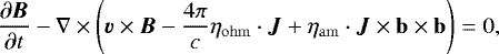 (13)
(13)
where b = B∕|B| the normalized magnetic field vector, J the electric current density vector, ηohm the ohmic diffusion coefficient and ηam the ambipolar diffusion coefficient.
2.2 Disk model
2.2.1 Initial conditions of the gas in the disk
The vertically integrated surface density profile Σ(r) was assumed to be a power law  with the reference surface density Σ0 at the characteristic radius r0 of the system and the volumetric gas density takes the form
![Mathematical equation: \begin{equation*}\rho(r, z) = \Theta_{\mathrm{H}}(r - r_{\mathrm{c}})\frac{\Sigma_0}{\sqrt{2 \pi} H(r)} \left(\frac{r}{r_0}\right)^{\mathrm{p}} \, \mathrm{exp} \left[\frac{1}{h^2} \left(\frac{r}{\sqrt{r^2 + z^2}} - 1\right)\right], \end{equation*}](/articles/aa/full_html/2022/03/aa42571-21/aa42571-21-eq14.png) (14)
(14)
where h = H∕r is the local aspect ratio and H = cs∕ΩK the gas scale height with the local isothermal sound speed  . Within a certain cutoff radius rc, we set the density to zero with a sharp transition and we thus mimiced a disk with an inner cavity of size rc. The transition is initially taken care of by the Heaviside function ΘH(r − rc) in Eq. (14). The sharp transition quickly softens and relaxes to the shape of a smooth inner rim during the simulation run after a few orbits. The cavity in the model was applied for both gas and dust.
In a simple blackbody disk being irradiated by stellar light with a grazing angle ϕ onto its surface, the temperature scales with radius as (Chiang & Goldreich 1997)
 (15)
(15)
where R*, T* and L* are the stellar radius, temperature and luminosity, respectively. The Stefan-Boltzmann constant is denoted by σSB. Thus, we assumed a radial power law profile for the temperature with T(r) = T0 r−q and the gas scale height scales with radius as  .
.
The initial values of the azimuthal gas velocity are slightly subkeplerian (Nelson et al. 2013):
 (16)
(16)
We assumed no initial velocities in the radial and polar direction, that is vr = vθ = 0.
2.2.2 Coronal gas structure
The hydrostatically stable coronal gas structure with density ρc (R) and pressure Pc(R) serves as a density floor throughout the simulation and prevents excessively low initial densities which prevents numerical instabilities. We used the same prescription as used in the previous models in Rodenkirch et al. (2020) based on Sheikhnezami et al. (2012).
The density was set to
 (17)
(17)
where ri is the radius at the inner boundary of the simulation domain and γ the adiabatic index. The corresponding pressure profile is given by:
 (18)
(18)
The density at the inner boundary ρc0(ri) is related to the disk’s density at the midplane and ri with the density contrast ![Mathematical equation: $\delta = \rho_{c0}(r_i) / \left[\Sigma(r_{\mathrm{i}}) / \left(\sqrt{2 \pi} H \right) \right]$](/articles/aa/full_html/2022/03/aa42571-21/aa42571-21-eq21.png) . Depending on Σ0, we set the density contrast to values ranging from δ = 10−7 to 5 × 10⁻⁷. In absence of X-ray/EUV heating, the gas temperature was directly set to the coronal temperature.
. Depending on Σ0, we set the density contrast to values ranging from δ = 10−7 to 5 × 10⁻⁷. In absence of X-ray/EUV heating, the gas temperature was directly set to the coronal temperature.
2.2.3 Dust structure
Vertical dust settling towards the midplane becomes more effective in the upper layers of the disk and the overall vertical thickness of the dust layer is over-estimated in models of a dust scale height uniquely depending on midplane values as in Dubrulle et al. (1995) (Dullemond & Dominik 2004). We therefore used the following vertical dust distribution
![Mathematical equation: \begin{equation*} \rho_{\mathrm{d}}(r, z) = \epsilon_{\mathrm{dg}} \, \rho(r, z) \left\{\frac{{\textrm{St}(r, z=0)}}{\alpha} \left[ \mathrm{exp}\left(\frac{z^2}{2 H^2} \right) - 1 \right] - \frac{z^2}{2 H^2} \right\} \end{equation*}](/articles/aa/full_html/2022/03/aa42571-21/aa42571-21-eq22.png) (19)
(19)
given in Fromang & Nelson (2009). The dust-to-gas mass ratio of the dust fluids is denoted by ϵdg and the dimensionless diffusion coefficient follows the α-viscosity prescription ν = αcsH (Shakura & Sunyaev 1973) with the kinematic viscosity ν. We assumed a constant value for the Schmidt number Sc = 1.
The initial azimuthal velocities were set to  . Similar to the gas, the initial radial and polar velocities of the dust fluids were set to zero.
2.2.4 Ionization rate
In all of the following models X-ray radiation was considered including both a radial and scattered component. The parametrization was based on the prescription of Igea & Glassgold (1999) and Bai & Goodman (2009):
![Mathematical equation: \begin{flalign} \zeta_{\mathrm{X}}=& \zeta_{\mathrm{X}, \mathrm{sca}}\left[\exp \left(-\frac{\Sigma_{\mathrm{top}}}{\Sigma_{1}}\right)^{0.65}+\exp \left(-\frac{\Sigma_{\mathrm{bot}}}{\Sigma_{1}}\right)^{0.65}\right]\left(\frac{R}{\mathrm{au}}\right)^{-2} \\ &+\zeta_{\mathrm{X}, \mathrm{rad}} \exp \left(\frac{\Sigma_{\mathrm{rad}}}{\Sigma_{2}}\right)^{0.4}\left(\frac{R}{\mathrm{au}}\right)^{-2} \nonumber. \end{flalign}](/articles/aa/full_html/2022/03/aa42571-21/aa42571-21-eq24.png) (20)
(20)
Both coefficients were multiplied by a factor of 20 compared to the cited values to model a fiducial X-ray luminosity of 2 × 1030 erg s−1 and were set to ζX,rad = 1.2 × 10⁻¹⁰ s−1 and ζX,sca = 2 × 10⁻¹⁴ s−1. The critical column densities accounted to Σ1 = 7 × 1023cm−2 and Σ2 = 1.5 × 1021 cm−2.
The luminosity increase was chosen to be compatible with the photoevaporation model of Ercolano et al. (2008); Picogna et al. (2019) where the luminosity LX = 2 × 1030 erg s−1 was used as the fiducial value. Taking into account the mass-luminosity relation presented in Flaischlen et al. (2021), Fig. 1 based on Getman et al. (2005), a luminosity of LX = 1 × 1029 erg s−1 would correspond in average to a M*≈ 0.15 M⊙ star. The increased value is thus better suited for the T Tauri star with M* = 0.7 M⊙ assumed in our model.
Additionally, the cosmic ray ionization rate ζcr was modeled by the parametrization of Umebayashi & Nakano (2009) where a characteristic column density of 96 g cm−2 was chosen. The symbols Σbot and Σtop refer to the column densities integrated along the polar direction, starting from the lower boundary (suffix bot)] and the upper boundary (suffix top). The radial column densities Σrad were computed starting from the radial inner boundary.
![Mathematical equation: \begin{flalign} \zeta_{\mathrm{cr}}=\;& 5 \times 10^{-18} \mathrm{~s}^{-1} \exp \left(-\frac{\Sigma_{\mathrm{top}}}{\Sigma_{\mathrm{cr}}}\right)\left[1+\left(\frac{\Sigma_{\mathrm{top}}}{\Sigma_{\mathrm{cr}}}\right)^{3 / 4}\right]^{-4 / 3} \\ &+\exp \left(-\frac{\Sigma_{\mathrm{bot}}}{\Sigma_{\mathrm{cr}}}\right)\left[1+\left(\frac{\Sigma_{\mathrm{bot}}}{\Sigma_{\mathrm{cr}}}\right)^{3 / 4}\right]^{-4 / 3}. \nonumber \end{flalign}](/articles/aa/full_html/2022/03/aa42571-21/aa42571-21-eq25.png) (21)
(21)
To account for short-lived radio nuclides in the disk, an ionization rate of ζnuc = 7 × 10⁻¹⁹ s−1 caused by the 26Al isotope (Umebayashi & Nakano 2009) acts as an ionization rate floor value. The resulting total ionization rate then simply sums up to ζ = ζX + ζcr + ζnuc.
2.2.5 Ionization fraction
We computed the ionization fraction of the gas via a semianalytical model for fractal dust aggregates elaborated by Okuzumi (2009). The main assumption here is an approximately Gaussian charge distribution in the dust grains. This approximation is reasonably well fulfilled if the dust aggregate consists of at least 400 monomers Dzyurkevich et al. (2013). In this approach, the ionization equilibrium was described by the following equations Okuzumi (2009):
![Mathematical equation: \begin{equation*} \frac{1}{1+\Gamma} - \left[ \frac{s_{\mathrm{i}} u_{\mathrm{i}}}{s_{\mathrm{e}} u_{\mathrm{e}}} \mathrm{exp}(\Gamma) + \frac{1}{\Theta} \frac{\Gamma g(\Gamma)}{\sqrt{1 + 2 g(\Gamma)} - 1} \right] = 0,\end{equation*}](/articles/aa/full_html/2022/03/aa42571-21/aa42571-21-eq26.png) (22)
(22)
with the parameter Θ:
 (23)
(23)
The function g(Γ) is evaluated as:
 (24)
(24)
After solving Eq. (22) numerically for Γ with a simple Newton-Raphson scheme, finally the ion and electron densities ni and ne can be calculated:
 (25)
(25)
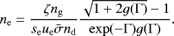 (26)
(26)
The stickingcoefficients si and se were set to 1 and 0.3 respectively, as described in Okuzumi (2009). The thermal ion and electron velocities ui,e follow:
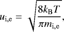 (27)
(27)
where me describes the electron mass and the ion mass is set to mi = 24 mp, corresponding to magnesium.
With the assumption of fractal dust aggregate with a dimension of D = 2, the dust aggregate size becomes ã = a0N1∕2 with the number of monomers N of size a0. Similarly, the geometric cross section  of these aggregates can be expressed as
  . The dust number density nd can be calculated as
 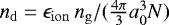 with the dust-to-gas ratio ϵion used in the ionization model.
In the limit of a vanishing dust-to-gas mass ratio the ionization fraction xe approaches
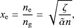 (28)
(28)
where ζ is the total ionization rate,  the dissociative recombination rate coefficient and n the neutral number density of the molecular species (Oppenheimer & Dalgarno 1974; Ilgner & Nelson 2006).
In the same manner as described in Bai (2017), we increased the ionization fraction in the wind region as a proxy for the effect of FUV-radiation:
![Mathematical equation: \begin{equation*} x_{\mathrm{fuv}} = 2 \times 10^{-5} \mathrm{exp}\left[-\left(\frac{\Sigma_{\mathrm{rad}}}{\Sigma_{\mathrm{fuv}}}\right)^4 + \frac{0.3 \Sigma_{\mathrm{fuv}}}{\Sigma_{\mathrm{rad}} + 0.03 \Sigma_{\mathrm{fuv}}} \right]. \end{equation*}](/articles/aa/full_html/2022/03/aa42571-21/aa42571-21-eq37.png) (29)
(29)
Simulations and key parameters.
2.2.6 Magnetic field
The magnetic field was set such that the initial plasma beta β at the midplane is independent of the radius r. The poloidal field was initialized from the vector potential Aϕ
![Mathematical equation: \begin{equation*} A_{\phi}(r, \theta) = \sqrt{\frac{8\pi P}{\beta}} \left(\frac{r}{r_0}\right)^{\frac{2p + q + 1}{4}} \left[1 + m \cdot \mathrm{tan}\left(\theta\right)^{-2}\right]^{-\frac{5}{8}} \end{equation*}](/articles/aa/full_html/2022/03/aa42571-21/aa42571-21-eq38.png) (30)
(30)
described in Bai (2017) and exhibits an outward-bent, hourglass shape depending on the parameter m where m = 0 would correspond to a completely vertical field. In order to avoid excessively small time steps in the low density regions close to the rotation axis, we limited the local Alfvén velocity  to 18vK(r0) by increasing the density in the cell accordingly, similar to Riols & Lesur (2018). This procedure does not affect the bulk of the wind flow.
2.2.7 Nonideal MHD
Using the electron fraction xe, the local ohmic diffusion coefficient ηohm can be written as (Blaes & Balbus 1994):
 (31)
(31)
where mn and me are the neutral and electron mass respectively. The electron-neutral collision frequency was set to  (Draine et al. 1983). The ambipolar diffusion coefficient ηam becomes:
 (32)
(32)
The ion-neutral collision rate was set to  (Draine et al. 1983). Since large diffusivities severely limited the simulation time step a super time stepping scheme was implemented and more details are given in Appendix C. We furthermore limited the magnetic Reynolds number for ambipolar diffusion Rm = cs H∕ηam to Rm ≥ 0.05, similar to Gressel et al. (2015), confirming that this approximation does not significantly alter the simulation outcome.
2.2.8 Heating and cooling
We employed the same temperature presciption as described in Rodenkirch et al. (2020) based on Picogna et al. (2019) to mimic the outflow due to photoevaporation in the simulation runs modeling a warm (magneto-) photoevaporative wind. According to their model, XEUV heating is significant up to radial column densities of Σr,crit = 2.5 × 1022 cm−2. In these regions, the temperatures Tphoto were updated to the values given by Eq. (1) in Picogna et al. (2019). Beyond the critical column density Σr,crit the temperature was cooled to the original gas temperature T0 = Tg.
In the case of the cold magnetic wind model b4c2np (see Table 1), the temperature in the corona was only slightly increased by 20% compared to the bulk temperature in the disk. We used a simple β-cooling recipe in the whole simulation domain to exponentially damp the temperatures to T0 on a time scale βcool
 (33)
(33)
2.3 Boundary conditions
We employed simple symmetric boundary conditions for most of the variables and boundaries where the values of the active cells are copied to the ghost cells. At the inner radial boundary, the radial velocity followed an outflow boundary condition where vr = 0 in the ghost zone if vr > 0 in the active cell. In the contrary case, vr was copied to the ghost cell. The same procedure was applied to the outer radial boundary with the opposite sign. With this formulation mass influx from outside of the domain was avoided.
At the θmin and θmax boundaries vϕ, vθ, Bϕ, Bθ and the EMF in radial direction change sign in the ghost zone to mimic a polar boundary. In MHD disk models the radial inner boundary condition can lead to spurious effects in the simulation domain. The same applies to the outer radial boundary where, if ill defined, artificial collimation affects the flow (Ustyugova et al. 1999). To avoid these difficulties we added a zone with additional artificial ohmic diffusion, so that the coupling between the gas and the magnetic field is weak enough that spurious effects were damped and the simulation domain remained largely unaffected. A similar approach was used at the inner boundary in Cui & Bai (2021) to stabilize the inner region of the domain.
Dimensionless values of the artificial ohmic resistivity ware ηohm,in = 2 × 10⁻⁴ and ηohm,out = 1 × 101 at the inner and outer damping zone, respectively. The extent of the damping zones is 10% of the inner and outer radius. With the choice of these values we found that the simulation domain and the timestep are largely unaffected by the boundary conditions. Adding an inner cavity with greatly reduced amount of gas and dust furthermore ensures negligible impact of the inner boundary condition on the wind flow.
2.4 Radiative transfer model and post-processing
We post-processed the dust density outputs with the radiative transfer code RADMC-3D (Dullemond et al. 2012). In order to obtain three dimensional dust density distributions the axisymmetric simulation outputs were extended in the azimuthal direction by repeating the densities in 300 cells in ϕ. For the thermal Monte-Carlo step and the image reconstruction with scattered light nphot = 106 and nphot_scat = 108 photon packages were used, respectively.
The thermal Monte-Carlo calculation was based on a modified version of the Bjorkman–Wood method (Bjorkman & Wood 2001) and the resulting temperatures were used in the synthetic images instead of the temperature profile prescribed in the MHD simulations. Every synthetic observation was created with only one dust species since the limited number of fluid would lead to artificial discrete step-like features in the image. Only considering one dust species at a time may lead to unrealistic temperature profiles but after checking the output of the thermal calculation of RADMC-3D the temperatures agreed with the dust temperature estimated computed in Appendix A in the relevant regions. We further emphasize that the synthetic images were produced in the H-band at a wavelength of 1.6 μm where scattered light effects dominate and thermal emission from the dust grains at these low temperatures is negligible.
The dust opacities were computed with optool (Dominik et al. 2021) and are similar to the DIANA opacities (Woitke et al. 2016) with a material mixture of 87% pyroxene, 13% carbon (by mass) but with an increased porosity of 64% to be consistent with a dust material density of ρmat = 1 g cm−3 in the simulations. Concerning the dust grain sizes, we computed the opacities for a1 = 0.1 μm, a2 = 1 μm and a3 = 10 μm corresponding to the dust sizes in the simulations. Anisotropic scattering effects were included by using the Henyey-Greenstein phase function approximation (Henyey & Greenstein 1941). A classical T Tauri star (CTT) was assumed with a temperature of T* = 4000 K and a radial extent of R* = 2.55 R⊙ at a distance of 150 pc which is in the range of typical properties of observed CTTs (Alcalá et al. 2021). The resulting images were convolved with a gaussian beam size of 75 mas to account for typical observational resolution limits using VLT/SPHERE (Beuzit et al. 2019; Avenhaus et al. 2018).
3 Results
Section 3.1 describes the relevant parameters and simulation runs. In the following subsections we present the simulation results starting with a description of the wind flow structure emerging from the disk in Sect. 3.2 and continue with the dust dynamics in Sect. 3.3. The effectiveness of dust entrainment and the outflow angle of the grains is addressed in Sect. 3.4, Sect. 3.5 and Sect. 3.6. Finally, in Sect. 3.7 we compare synthetic observations computed from the simulation output with existing observations.
3.1 Parameters and normalization
Table 1 summarizes the key parameters of the different simulation runs presented in this study. The first part of the label describes wether a magnetic wind (for instance b4 with β = 104) or a photoevaporative wind without magnetic fields was modeled (with label ph). Subsequently, the letter “c” refers to the cavity location (such as c2 for a cavity at 2 au). The sublabels np, a3 and eps2 refer to “no photoevaporation”, α = 10−3 and ϵion = 10−2, respectively.
In the code all quantities were treated in dimensionless units that are scaled as follows:

where the length unit was set to r0 = 5.2 au, the semi-major axis of Jupiter as a natural scale of stellar systems. The initial density profile was scaled to reach a surface density of Σ = 200 g cm−2 at r = 1 au and decreases radially with power law slope of p = 1. The central star mass was set to 0.7 M⊙ and the disk follows a moderate aspect ratio of  which corresponds to a flared disk with a temperature slope of q = 1∕2. These parameters correspond to a stellar luminosity of L* = 1.5 L⊙ with the assumption of a grazing angle of ϕ = 0.02. The luminosity is in line with the stellar parameters of T* = 4000 K and R* = 2.55 R⊙ mentioned in Sect. 2.4.
A temperature floor of Tmin = 10 K and a cooling time scale of βcool = 10−4 was applied. The fiducial value of the inner cavity size was chosen to be rc = 2 au. Further parameters are the adiabatic index of γ = 5∕3 corresponding to an ideal atomic gas and the mean molecular weight μ = 1.37125, consistent with the value chosen in Picogna et al. (2019) for the composition of the ISM (Hildebrand 1983).
In Sect. 2.2.5, the model necessitates an assumption of the dust content in the disk. In this work the ionization model was parametrized with a static value of the dust-to-gas ratio ϵion = 10−3 and a monomer size of a0 = 5 μm that constitute aggregates with 400 particles, resulting in a grain size of 100 μm. Increasing the dust-to-gas ratio by one order of magnitude did not alter the ionization fraction profile by a great amount, as described in Appendix B. In order to simplify the model, the dynamically simulated dust fluids were not coupled to the ionization model and the relative insensitivity to the chosen parameters in the midplane supports this approximation.
All simulation runs were carried out with three dust species of the sized a = 0.1 μm, 1 μm and 10 μm, intended to represent the three cases of full entrainment, slow decoupling, and fast decoupling from the gas in the wind. The material density of the grains was set to ρmat = 1 g cm−3.
The computational grid adopts a spherical symmetry and contains 500 logarithmically spaced cells in radial direction whereas 276 cells were used in the polar (θ) direction. Inorder to increase the vertical resolution closer to the disk mid plane, the polar cells were arranged in a stretched grid, with a cell size atthe polar boundaries that was twice as larger compared to the mid plane. With this approach a resolution of 7 cells per H in polar direction at r = r0, z = 0 was reached. To avoid numerical issues at the polar boundaries the grid limits in this direction were chosen such that θmin ≈ 87 ° and θmax ≈−87 °. The radial domain spans from 1 au to 200 au as indicated in Table 1.
3.2 Gas flow structure
Figure 1 visualizes the gas wind flow for the simulation runs phc2, b5c2 and b4c2. The latter two include magnetic fields whereas the former only includes the photoevaporation recipe. Comparing both magnetic winds in Fig. 1 the magnetic field structure consists mostly of straight field lines for β =104, whereas the weaker field shown in the central panel exposes a more irregular field structure towards the inner region of the disk. For this field strength and configuration, the wind is in the transition between a thermally dominated and a magnetically dominated wind. We note that these are simulation snapshots and not averaged wind flows.
In terms of wind total mass loss rates all of these three runs display similar results, as shown in Fig. 2. Generally, the wind converges to a steady-state flow after a time scale about 200 orbits at 1 au and the simulation time chosen for these runs is thus sufficient to explore relevant wind dynamics in the inner region.
The sharp cutoff of the disk at r = 2 au quickly relaxes towards a stable equilibrium after a few orbits. The choice of the initial shape of the inner rim is thus not relevant for the windflow. We observe accretion of gas through the inner cavity when a magnetic field is present. This effect, which can be best observed in the right panel of Fig. 1, is more pronounced for larger magnetic field strengths and is caused by wind-driven accretion.
The photoevaporation gas mass loss rates reach ≈2.83 × 10⁻⁸ M⊙ yr−1, in good agreement with Picogna et al. (2019). The mass loss rates in the simulation runs b5c2 and b4c2 are ≈ 3.13 × 10⁻⁸ M⊙ yr−1 and ≈ 3.03 × 10⁻⁸ M⊙ yr−1, respectively. In the case of apurely magnetically driven wind without any heating by ionizing radiation of model b4c2np the wind mass loss rates are similar with a value of 3.19 × 10⁻⁸ M⊙ yr−1. The mass loss rates were computed at 95% of the outer radial simulation boundary. The region within five gas scale heights of the disk was excluded from the mass loss rate to avoid the corruption of the results from circulation within the disk.
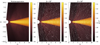 |
Fig. 1 Gas density maps of the simulations phc2, b5c2 and b4c2 after 500 orbits at 1 au. Magnetic field lines are represented by the white lines in the corresponding panels. The color map scaled logarithmically annotated by the exponent to a base of ten and represents the volume density of the gas in g cm−3. |
 |
Fig. 2 Total wind mass loss rates of gas and dust for the simulation runs phc2, b5c2, b4c2 and b4c2np. Results from 10 μm grains are excluded due to the negligible outflow and the lack of entrainment in the wind for all runs shown above. |
3.3 Dust flow structure
In Fig. 3 the dust flows are shown for the grain sizes 0.1 μm, 1 μm and 10 μm. Generally, 10 μm sized grains are hardly entrained with the wind flow since the drag force is too weak to counter act the gravitational pull. 0.1 μm grains are well coupled to the gas flow and can be considered as tracers of the wind. Throughout the analysis we refer to the flow angle or inclination angle, meaning the angle enclosed between the dust flow direction and this disk mid plane axis at z = 0. The inclinations θd of the dust flows are smaller in terms of latitude for the thermally driven wind shown on the left-hand side compared to the magnetically driven wind on the right-hand side. The magnetic field is well coupled to the gas in the wind region where the ionization fraction xe,i surpasses 10−4 and the field topology forces the wind flow to be more inclined compared to the thermally driven wind.
The same phenomenon also appears for 1 μm grains shown in the second row of Fig. 3. Due to the weaker coupling and the lack of pressure support the dust flow is less inclined with respect to the gaseous wind compared to smaller grains. The dust flow exhibits wave-like patterns in the case of β = 105 and becomes more stable for larger magnetic field strengths. These wave structures coincide with the irregular magnetic field patterns displayed in Fig. 1. We furthermore point out that the dust flow consisting of 1 μm grains is efficiently launched in the inner part of the disk, whereas beyond several au the wind significantly weakens. The dusty wind cannot be sustained in the lower density regions further out and up in the disk since the Stokes number significantly increases.
An example of a dust flow in a cold magnetically driven wind is given in Fig. 4 for an initial β = 104. The inclination with respect to the mid plane is smaller compared to the warm magnetothermal or photoevaporative winds. Grains with a size of 1 μm are entrained at a rather shallow inclination angle and similar to the warm winds, dust entrainment is negligible considering 10 μm dust particles. While material in the winds including photoevaporation is ejected with a velocity of ≈ 15 km s−1 the outflow velocity of the cold magnetic wind in b4c2np only reaches values of ≈ 5 km s−1. The decreased wind speed causes a smaller drag force between gas and thus lowers the dust entrainment efficiency. Given that the mass loss rate is approximately equal to the one of the heated winds, the gas and dust densities in the wind region are significantly higher.
In Fig. 5, the cumulative mass loss rate depending on the cylindrical radius of the foot point of the wind is shown. The wind streamlines were traced backwards from the cells close to the outer radial boundary and the foot point was registered when the streamlines crosses the surface at five gas pressure scale heights. Only streamlines with foot point rf ≥ 3 au were considered since the wind flow structure and the limited resolution did not in every case ensure a successful construction of traceable streamlines close to the inner cavity. The mass loss rates were obtained from a velocity and density field averaged over 50 orbits at 1 au starting from 600 orbits.
Warm magnetic winds lead to more dust entrainment and a stronger magnetic field increases the dust mass loss rate significantly. The dashed lines in Fig. 5 mark the radius within from within 99% of the mass loss occurs, which illustrate less efficient dust entrainment for larger grains further out in the disk. Numerical values are 32.3 au, 34.5 au, 43 au and 88.8 au for the simulations phc2, b5c2, b4c2, b4c2a3 and 0.1 μm grains, respectively. Analogously, the limits for 1 μm grains are 14.6 au, 12.7 au, 14.6 au and 44.3 au. The general trend is that the dust grains are preferably entrained starting from the inner regions of the disk. The limiting radius decreases with increasing dust size and hence we expect a much larger ejection region of dust for the smallest grain size. Considering the results of the simulation b4c2a3 with an increased viscosity of one order of magnitude (α = 10−3) the limiting radius lies significantly further outward. Increased turbulent diffusion effectively transports dust grains towards the wind launching front at larger radii.
Going back to Fig. 2 the mass loss rate for the two relevant dust species stabilizes over a few hundred orbits in the case of a thermal wind. In the case of magnetically driven winds however, dust mass loss rates reach a quasi-steady state but are slowly increasing throughout the simulation. In the presence of a cold magnetic wind, the mass loss rates of larger micron-sized dust grains are lower compared to the ionized winds since the flow angle is rather shallow and the entrainment efficiency suffers from the decreased wind speed.
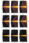 |
Fig. 3 Dust density maps for the simulations phc2, b5c2 and b4c2 after 500 orbits at 1 au. Dust velocity streamlines are annotated by the white arrowed lines. The upper, center and lower three panels visualize the flow of grains with size 0.1 μm, 1 μm and 10 μm, respectively. |
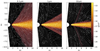 |
Fig. 4 Dust density maps for the simulation b4c2np after 500 orbits at 1 au. Dust velocity streamlines are annotated by the white arrowed lines. |
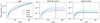 |
Fig. 5 Cumulative mass loss rates of gas and dust for the simulation runs phc2, b5c2, b4c2 and b4c2a3 starting from 3 au. The cylindrical radius or foot point of the loss is obtained by tracing backwards the corresponding streamline from the outer radial boundary down to 5 scale heights above the disk mid plane. The flow field is averaged over 50 orbits at 1 au starting at 600 orbits. The vertical dashed lines mark the limit of the region where 99% of the mass loss occurred. |
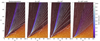 |
Fig. 6 Numerically integrated dust trajectories for snapshots after 500 T0 of the simulation runs phc2, b5c2 and b4c2. The orange color map represents the gas density and the thin arrowed white lines denote the gas velocity streamlines. The thicker colored lines visualize the dust trajectories for grain sizes ranging from 0.1 μm to 10 μm. |
3.4 Maximum grain size and flow angle
In order to quantify the maximum entrained grain size and the entrainment angle, we chose the approach to numerically integrate streamlines of various dust species based on the gas velocity field from the simulations. The following system of equation was solved numerically with the given velocity field of the corresponding simulation output:
![Mathematical equation: \begin{flalign} v_{\mathrm{d, r}} & = v_{\mathrm{d}, \phi} - \frac{GM_*}{\left(r^2 + z^2\right)^{rac{3}{2}}} r - \frac{v_{\mathrm{d, r}} - v_{\mathrm{g, r}}}{t_{\mathrm{s}}}, \\ v_{\mathrm{{d], z}}} &= - \frac{GM_*}{\left(r^2 + z^2\right)^{\frac{3}{2}}} z - \frac{v_{\mathrm{{d}, z}} - v_{\mathrm{g, z}}}{t_{\mathrm{s}}}. \end{flalign}](/articles/aa/full_html/2022/03/aa42571-21/aa42571-21-eq48.png)
The numerical integration was carried out with the VODE solver Brown et al. (1989). We verified that the streamlines were comparable to the ones in the dust velocity field output from the simulation. No significant deviations were visible.
The results are shown in Fig. 6 for 20 logarithmically distributed grain sizes ranging from 0.1 μm to 10 μm. The resulting trajectories match the corresponding dust streamlines from the actual simulation. As the starting point we chose r = 8 au, z = 2.5 au which is situated well above the wind launching front. As expected from the simulation outputs 10 μm grains fall back towards the disk surface in the case of winds including photoevaporation (models phc2, b5c2 and b4c2). Generally, grains are lifted more efficiently in the case of warm, magnetic winds. Grains larger than ≈ 3 μm to 4 μm are lifted further but eventually fall back onto the disk at larger radii in the presence of a thermal wind.
For warm, magnetically driven winds, the limiting grain size shifts towards ≈ 6 μm. In a cold, magnetic wind the picture changes and only submicron dust grains are lifted far from the disk surface and particles larger than 1 μm fall back onto the disk or are not entrained at all. The decreased wind speed is responsible for the lower dust entrainment efficiency as mentioned in Sect. 3.3.
Since the dust flow inclination angle is strongly dependent on the grain size, we quantified the inclination by fitting linear functions to the dust trajectories presented in Fig. 6. We only considered the final 25% part of the cylindrical radius of the trajectory for the fits. The corresponding slopes and inclination angles based on the simulations phc2, b5c2, b4c2 and b4c2np are plotted in Fig. 7. For small grains and warm winds the difference in the inclination angle is rather small. The inclination of the flow of 1 μm grains ranges from roughly 67° to 69 °. Considering 3 μm grains however, the inclination angle is 36.1° assuming a thermal wind compared magnetic winds with 44.4° and 46.5° for β = 105 and β = 104, respectively.Generally, the inclination angle is larger for warm, magnetic winds, especially considering micron sized grains.
A significant difference in inclination is however observed in a cold magnetic wind. While 0.1 μm-sized dust grains are entrained by an angle of 59.1°, the inclination drops down rapidly to roughly 25° for micron-sized grains, as expected.
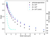 |
Fig. 7 Asymptotic dust flow inclination depending on the grain size for the simulation runs phc2, b5c2, b4c2 and b4c2np. |
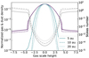 |
Fig. 8 Normalized vertical density slices of the phc2 at different radial locations in the disk. The violet lines represent the normalized gas density while the turquoise lines display the dust density of 10 μm grains. The gray lines denote the respective Stokes number profile. |
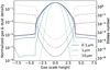 |
Fig. 9 Normalized vertical density slices and Stokes number profiles of the phc2 similar to Fig. 8 for the grain sizes 0.1 μm (straight lines), 1 μm (dashed lines), 10 μm (dotted lines) at 5 au. |
3.5 Wind launching surface
Since the dust entrainment efficiency seems to be dependent on the dust reservoir at the location of the foot point of the wind, we therefore provide a more detailed analysis of the radial dependencies of the dust entrainment efficiency in this subsection.
We only focus on winds including photoevaporation where the wind launching surface is marked by a sharp transition in the gas density. Figures 8 and 9 visualize vertical slices of normalized gas and dust densities as well as the respective Stokes number profile. As expected, in Fig. 8 the dust scale height of 10 μm sized grains narrows with increasing radius as the Stokes number within the bulk of the disk increases due to the negative radial density slope. The kink at roughly 4.5 gas scale heights represents the wind launching surface. Clearly, the dust scale height is too small to lift a considerable amount of grains to the launching surface, especially at larger radii.
A comparison between the different dust species at 5 au is given in Fig. 9. The trend of larger dust scale heights with smaller Stokes numbers is readily visible. Weaker wind flows by several orders of magnitude appear for 1 μm sized grains compared to 0.1 μm particles. Only the vertical distribution of the smallest 0.1 μm grains that are well coupled to the gas appear to correspond the gas density distribution.
In the following, we aim to examine the dust entrainment efficiency depending on the radial location in the disk. We therefore traced various quantities, such as dust-to-gas ratio, Stokes number, temperature and gas number density along the wind launching surface. Numerically we defined this surface to be located about 0.3 gas scale heights above the kink in the vertical gas density profile in order to decrease the impact of fluctuations close to the surface of the disk. The kink location was determined by numerically evaluating local extrema in the second derivative of the vertical gas density profile which we find to be a robust method to find the launching surface.
The corresponding quantities at these positions are displayed in Fig. 10 where thermally and magnetically driven winds with 0.1 μm and 1 μm-sized grains are taken into account. Clearly, the dust entrainment efficiency, defined by the dust to gas ratio close to the wind launching front shown in the upper most panel of Fig. 10, decreases significantly with increasing radius. At the inner part of the flow close to the cavity at 2 au, 0.1 μm- sized grains are basically perfectly entrained with the wind for both photoevaporative and magnetically driven outflows since the initial dust-to-gas ratio is ϵdg = 10−2. In the outer part of the disk, the dust-to-gas ratio in the wind decreased by one to two orders of magnitude. For 1 μm-sized grains the effect is more pronounced with a decline of six orders of magnitude. It becomes apparent that generally the magnetically driven wind with β = 104, represented by the dotted lines, leads to a higher dust-to-gas ratio in the wind flow compared to weaker field strengths or a purely thermally driven wind.
One could argue that dust entrainment becomes less effective at larger radii because of the more diluted gas in the wind and thereby larger Stokes numbers. This is however not the case as shown in the second panel of Fig. 10. In the inner part of the disk up to ≈8 au to 9 au the Stokes number close to the launching surface increases until it stagnates and remains constant at the outer part of the disk. The decrease in dust entrainment efficiency can thus not be attributed to a weaker coupling between gas and dust in these regions. The gas density in the wind close to the launching surface indeed decreases with radius as shown in the bottom panel of Fig. 10. On the other hand, the gas temperature heated by the ionizing radiation from the central star in turn also decreases with radius. The peak in temperature is reached at ≈ 8 au to 9 au, agreeing with the stagnation point of the Stokes number profile. By linear fitting the quantities at the wind launching surface in logarithmic space we determine the power law slopes. Beyond 8 au the thermal velocity vth decreases ∝ r−0.13 whereas the gas density profile follows the power law ∝ r−1.41. Looking at the definition of the Stokes number in Eq. (8), we expect an approximately constant relation St ∝ ΩK∕(ρg ⋅ vth) ∝ r0.04 with a Keplerian angular frequency following ΩK ∝ r−1.5.
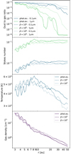 |
Fig. 10 Physical quantities at the wind launching surface of the simulation runs phc2 (straight lines), b5c2 (dashed lines) and b4c2 (dotted lines). In the top two panels the blue lines represent 0.1 μm -sized grains, whereas the green lines denote 1 μm-sized grains. |
 |
Fig. 11 Streamlines starting from r = 8 au, z = 2.5 au. Shown are poloidal velocities of gas and dust along the streamline (left two panels) and the respective Stokes numbers St as well as the Alfvén Mach number MA (right two panels). |
3.6 Gas and dust streamlines
In Fig. 11 velocities, Stokes number and Alfvén Mach number are plotted for a representative streamline starting at r= 8 au. Since the flow is close to a steady state we can consider the streamline as a proxy for the actual trajectory of a dust and gas parcel moving in the wind. The radial velocities in the left-most panel are almost constant with the cylindrical radius whereas the vertical velocities in z-direction significantly increase up to values on the order of 15 km s−1. The models including magnetic effects generally lead to slightly faster wind flows increasing with the magnetic field strength. Depending on the dust grain size the velocity can be significantly less compared to the gas velocity, differing by roughly 5 kms−1. Dust velocities are also consistently faster in the magnetic wind case. Looking at the Stokes numbers of the two smallest dust species, the values up to unity are reached for micron-sized grains far from the disk. The right-most panel demonstrates that the wind is onlysubalfvénic for a small part close to the wind launching front. Even in the simulation run b4c2 with an initial β =104 the wind quickly reaches superalfvénic speeds which in consequence represents a small magnetic lever arm. This picture is in line with recent models of magnetothermal winds such as Gressel et al. (2015); Bai (2017); Rodenkirch et al. (2020).
3.7 Synthetic observations
Given that the wind flow is rather thin and dust is not perfectly entrained for larger grain sizes and distances from the central star, the observability of such dusty winds deserves a closer look. As a first simple estimate we computed the radial optical depth depending on the latitude θ. The results are displayed in Fig. 12 for three dust species ranging from 0.1 μm to 10 μm in the H-band. The optical depth τobs,i of dust species i was calculated by
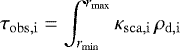 (39)
(39)
with the scattering opacity κsca,i. The inner and outer radial boundaries are denoted by rmin and rmax, respectively.In Fig. 12, the bulk of the disk appears to be optically thick for all dust species in the H-band. The wind itself however is optically thin throughout the whole flow and its optical depth reaches values of τobs≈ 10−1 in the direction of the wind base. Naturally, the optical depth decreases with larger viewing angles due to the thinner dust and gas density in these regions.
For 1 μm-sized grains the optical depth is comparable to the one for 0.1 μm grains but tapers off at a flatter angle of 70° due to the less inclined dust flow. Finally, the larger 10 μm grains are almost irrelevant since dust entrainment is negligible and the densities are therefore approaching the dust density floor value. In Figs. 13 and 14, synthetic observations are shown with inclination angles of 20 ° and 0° in latitude, respectively. In comparison to the disk brightness the wind structure can be clearly identified as an hourglass-shaped signature. Smaller 0.1 μm grains are confined to a narrower cone with diffuse emission towards the outer regions. A rather sharp transition between the region devoid of dust close to the rotation axis and the inner most part of the dusty wind is visible.
The wind is not completely illuminated by the stellar light because of the decreasing dust content towards the outer regions of the disk. Comparing the morphology of the scattered light signatures from 0.1 μm grains to emission of 1 μm grains, the larger dust particles lead to a conical shape with a wider opening angle with respect to the rotation axis. This feature is expected from Fig. 7 where the increased grain size leads to weaker gas-dust coupling and therefore causes a dust flow with a smaller inclination. In addition, larger grains are entrained less efficiently in the outer regions of the disk compared to smaller grains, due to the stronger dust settling towards the disk mid plane. In combination with the larger opening angle of the flow we therefore detect a less diffuse, conical shape with a sharp transition in brightness towards the outer regions of the disk.
It is also visible that magnetic winds with stronger fields confine the dust flow more towards the rotation axis and exhibit a larger inclination angle of the dust flow. The cold MHD wind model exhibits a brighter wind region compared to the models including photoevaporation. As expected, the opening angle of the 0.1 μm wind flow is larger compared to the warm wind models and resembles the emission of 1 μm if photoevaporative heating is included. In the cold wind model 1 μm-sized grains are entrained in a shallow inclination angle and could be identified as a disk with a larger aspect ratio than the thermodynamics would otherwise allow in the system. At a viewing angle of 20 ° the backside of the disk almost shadows the dusty wind, making it difficult to identify such a dusty outflow on the basis of a low resolution or a low signal-to-noise ratio. Generally, we find the brightness contrast between wind and disk to be less in the case of 1 μm grains if the viewing angle is 20°. In the edge-on view shown in Fig. 14, the wind signature brightness is comparable to the disk brightness for both grain sizes.
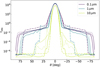 |
Fig. 12 H-band radial optical depth τobs originating from the central star depending on the inclination expressed in latitude for three dust species with sizes 0.1 μm, 1 μm and 10 μm indicated by the color scheme. The continuous lines refer to the photoevaporation simulation phc2, the dashed lines to the magnetic wind b5c2 with β = 105 and the dotted lines to the run b4c2 with β = 104. |
4 Discussion
In the following, we discuss limitations of our wind model and compare the key results with other works in the literature. An advantage of the fluid description over a Lagrangian particle formulation of the dust dynamics in the simulations, is the ability to resolve low density regions if a large density contrast between the midplane and the corona as well as the wind is present, which is the case in the disk-wind system shown here. The disadvantage is the lack of proper modeling of a dust grain size distribution. A single-size dust population is unlikely due to dust growth and fragmentation. The synthetic observations thus only serve as a hint towards the detectability of dusty winds and the expected shape of the flow assuming the corresponding predominant dust size. Including multiple dust fluids in the synthetic observations would lead to misleading structures in the emission because of the rather sharp transition between the inner dust free cone and the wind region.
Deducing the maximum dust grain size from the wind flow angle seems to be rather difficult since the underlying parameter space is degenerate. On the one hand, the opening angle of the dusty wind increases with the grain size. On the other hand, the same effect occurs with colder magnetically driven winds. A distinction could be made by probing the wind speed, which is smaller in the cold wind case, albeit being a specific example.
If the wind is optically thin for the ionizing radiation of the central star, the difference between photoevaporative winds and warm magnetically driven winds is minor. In future works, the parameter space could be extended by varying the luminosity of the central star and by using a more sophisticated photoevaporation model as presented in Ercolano et al. (2021); Picogna et al. (2021).
Within the simulated time frame we do not observe any significant asymmetry between the upper and lower wind. Such asymmetric flows were observed in simulations by Béthune et al. (2017), Suriano et al. (2018) and Riols & Lesur (2018). Ring formation by magnetically driven winds does not occur in our simulation runs compared to Suriano et al. (2018) and Riols & Lesur (2018) where ambipolar diffusion is prescribed to be the dominant nonideal MHD effect. In their work however, larger field strength in the regime of β = 103 were probed. Riols & Lesur (2018) also observed ring formation for β = 104 and included fluid dust focusing on the dust dynamics in the mid plane.
Given that the same photoevaporation recipe is used in this paper as the one in Franz et al. (2020) our results are compatible in this regime. They conclude a maximum entrainable grain size of 11 μm. As shown in Fig. 6 our photoevaporative models allow a short-term lifting of 10 μm dust grains which eventually fall back onto the disk. In the complete dust fluid picture, the small dust grain scale height prevents any dust entrainment starting from the wind launching front. More recently, Franz et al. (2022) studied the observability of dust entrainment in photoevaporative winds based on their models in Franz et al. (2020). They conclude that the wind signature in scattered light is too faint to be observed with SPHERE IRDIS, but might be detectable with the JWST NIRCam under optical conditions. In their synthetic observations a similar “chimney”-shaped wind emission is visible compared to our photoevaporative models.
Giacalone et al. (2019) found a positive correlation between gas temperature and maximum dust grain size in their semi-analytical magneto-centrifugal wind model which corresponds best to our cold magnetically driven wind model b4c2np. Our results corroborate their findings of a maximum entrainable dust size in the submicron regime in a cold wind around a typical T Tauri star. Our models including photoevaporation furthermore agree with Hutchison et al. (2016a) where the maximum grain size was determined to be < 10 μm depending on the disk radius for a typical T Tauri star. They additionally argue that dust settling most certainly limits this maximum size further, which we confirm in our models, where the diminishing dust entrainment efficiency can be attributed to the dust settling towards the mid plane.
In recent scattered light observations of RY Tau (Garufi et al. 2019), a broad dusty outflow obstructing the underlying disk was detected. Both lobes are inclined by roughly 45 °. The presence of a jet in this system advocates a magnetic wind launching mechanism that causes the features observed in the near-infrared. We do not observe an optically thick wind that would be able to completely obstruct the disk, since the dust densities are too low, especially in the models including photoevaporation. A possibility might hence be a slow, cold, magnetic wind at higher field strengths. The large opening angle in the observation would suggest a wind flow containing dust grains of the size of several μm if photoevaporation would be the significant wind mechanism. If a cold magnetically driven wind was the dominant factor, smaller submicron grains would be the solution compatible with our models.
In this work, we neglected the effect of radiation pressure that may be able to blow out small dust grains. Franz et al. (2020) argued that a photoevaporative wind can entrain grains of sizes roughly 20 times larger compared to a compatible radiation pressure model from Owen & Kollmeier (2019). Since we use similar parameters for the photoevaporation model, the effect of radiation pressure should not significantly affect the dust dynamics in the studied parameter space.
In the photoevaporation models, the gaseous part of the wind reaches temperatures of up to 104 K. We verified thatthe dust temperature stays below the dust sublimation temperature in Appendix A.
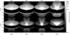 |
Fig. 13 Radiative transfer images in the H-band (λ = 1.6 μm) of simulation runs with photoevaporation (left most column), β = 105 (center left column), β = 104 (center right column) and a cold magnetic wind with β = 104 (right most column). The upper panels are based on dust grains with a = 0.1 μm whereas the lower panels demonstrate synthetic images with a = 1 μm. The object is modeled at a distance of 150 pc with a solar type star at an inclination of 20°. |
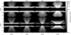 |
Fig. 14 Radiative transfer images in the H-band (λ = 1.6 μm) of the same simulation runs as in Fig. 13 but with an edge-on view at an inclination of 0°. |
5 Conclusion
We presented a suite of fully dynamic, global, multifluid simulations that model dust entrainment in photoevaporative as well as magnetically driven disk wind using the FARGO3D code. We demonstrated that both types of winds are able to efficiently transport dust in the wind flow and addressed the observability of such dusty winds with the help of the RADMC-3D radiative transfer code. In the following we summarize the main results:
-
The maximum entrainable dust grain size amax both depends on the type of the wind launching mechanism and the turbulent diffusivity of the disk. Whereas magnetic winds including XEUV-photoevaporation only show minor differences in amax, ranging from 3 μm to 6 μm, cold magnetically driven winds at comparable field strengths only entrain submicron sized grains efficiently.
-
With increasing radius the dust to gas ratio in the wind drops rapidly, mainly due to the smaller dust scale height in comparison to the gas scale height. Dust grains are unable to reach the wind launching surface in the outer regions of the disk and the dust content in the wind starting from these locations hence decreases. In the case of warm, ionized winds the Stokes number stays approximately constant with radius beyond 8°. Generally, magnetically driven winds including photoevaporation are slightly more efficient in entraining dust compared to pure photoevaporative flows.
-
The dust flow angle θd decreases with increasing grain size to the weaker coupling between gas and dust. In warm, ionized winds the flow angle reaches values of 67° ≤ θd ≤ 69° for a = 1 μm sized grains. At a grain size of a = 3 μm a photoevaporative dust flow provides θd ≈ 36° whereas a warm magnetic wind leads to a steeper dust flow with θd ≈ 45°. In a cold magnetic wind the flow angle is significantly smaller, being θd ≈ 59° for a = 0.1 μm and θd ≈ 25° for micron-sized grains.
-
Radiative transfer images in the H-band suggest a rather weak, optically thin emission for photoevaporative winds. A more pronounced, conical shape is visible considering 1 μm grains. The larger dust flow angle θd leads to a narrower emission region in the case of warm, ionized magnetic winds. Cold magnetic winds appear with a significantly larger opening angle with comparable grain sizes. The emission region of the wind appears brighter and more easily detectable due to the increased dust density of the slower magnetic wind.
Our results presented in this paper might help to constrain the magnetic field strength as well as the dominating wind mechanism if such dust signatures will be detected in future observations. The dust grain size could be determined via the inclination angle of the flow. Although the parameter space is degenerate, probing the wind speeds might help to differentiate between thermally and cold magnetically driven winds.
Acknowledgements
We would like to thank R. Franz for helpful discussions. We furthermore thank the anonymous referee for helpful comments that further improved the manuscript. Authors Rodenkirch and Dullemond acknowledge funding from the Deutsche Forschungsgemeinschaft (DFG, German Research Foundation) - 325594231 under grant DU 414/23-1. The authors acknowledge support by the High Performance and Cloud Computing Group at the Zentrum für Datenverarbeitung of the University of Tübingen, the state of Baden-Württemberg through bwHPC and the German Research Foundation (DFG) through grant INST 37/935-1 FUGG. Plots in this paper were made with the Python library matplotlib (Hunter 2007).
Appendix A Dust temperature estimate
The relatively high temperatures in the ionized wind models heat the dust grains that are entrained in the gas flow. We show in the following that dust particles do not reach the dust sublimation threshold and would thus remain solid along their trajectories. The expression of the heating rate per unit surface qd is described in Gombosi et al. (1986), taking into account both contact and friction heating. We follow the approach of Stammler & Dullemond (2014) in this regard and evaluate the subsequent expressions:
 (A.1)
(A.1)
where the heat transfer coefficient CH,d is expressed as
![Mathematical equation: \begin{equation*} C_{\mathrm{H, d}} = \frac{\gamma + 1}{\gamma - 1} \frac{k_{\mathrm{B}}}{8 \mu m_{\mathrm{p}} s^2} \left[\frac{s}{\sqrt{\pi}} \mathrm{exp}\left(-s^2\right) + \left(\frac{1}{2} + s^2\right) \mathrm{erf}\left(s\right)\right] \,, \end{equation*}](/articles/aa/full_html/2022/03/aa42571-21/aa42571-21-eq51.png) (A.2)
(A.2)
with the error function erf and the normalized difference between dust and gas velocities:
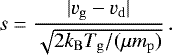 (A.3)
(A.3)
The recovery temperature Trec is given by the expression (Gombosi et al. 1986):
![Mathematical equation: \begin{equation*} T_{\mathrm{rec}} = \frac{T_{\mathrm{g}}}{\gamma - 1} \left[ 2\gamma + 2(\gamma - 1)s^2 - \frac{\gamma - 1}{\frac{1}{2} + s^2 + \frac{s}{\sqrt{\pi}} \mathrm{exp}\left(-s^2\right) \mathrm{erf}^{-1}\left(s\right) } \right] \,. \end{equation*}](/articles/aa/full_html/2022/03/aa42571-21/aa42571-21-eq53.png) (A.4)
(A.4)
The dust equilibrium temperature is then finally computed by solving
 (A.5)
(A.5)
with the thermal cooling efficiency factor
 (A.6)
(A.6)
using the Planck mean opacity κP with the corresponding temperature. Fig. A.1 provides the solutions of the equilibrium dust temperatures in comparison with the gas temperatures in a photoevaporative flow including 0.1 μm grains. We assume a sun-like star in the computation and find maximum dust temperatures of Td ≈ 345 K at a radial distance of r = 2 au. Due to the thin gas in the wind region the ambient heating has an almost negligible impact on the dust temperature. Without the flux of the central star the dust grains would reach Td ≈ 40 K only being heated by the ionized gas. In the wind flows presented here dust temperatures are clearly below the dust sublimation threshold which would be ≈ 980 K assuming pyroxene as the grain material embedded in a thin medium of the density ρg = 1 × 10⁻¹⁶ g cm−3 (Pollack et al. 1994).
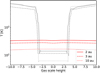 |
Fig. A.1 Vertical slices of gas and dust temperatures at different radial location in the disk and wind region of the photoevaporation simulation phc2. The gray lines represent the gas temperatures whereas the red lines display the equilibrium dust temperatures of the 0.1 μm grains. |
Appendix B Ionization fraction
Since the ionization fraction depends on the dust-to-gas ratio ϵion in the disk a comparison between ϵion = 10−3 and ϵion = 10−2 of the simulation runs b4c2 and b4c2eps2 is shown in Fig. B.1. The ionization is relatively insensitive to the increased dust-to-gas ratio and only decreases by a small amount in the weakly ionized disk mid plane. In the dust density slice the effects are negligible.
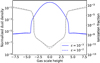 |
Fig. B.1 Normalized dust density (blue lines) and ionization fraction (gray lines) in the simulations b4c2 and b4c2eps2 with a dust-to-gas ratio of ϵ = 10−3 and ϵ =10−2, respectively. The snapshot is taken after 1000 orbits at 1 au. |
Appendix C Super time stepping
This sectiondescribes the implementation of the Super Time-Stepping technique (STS) for parabolic or mixed advection-diffusion problems. Introduced by Alexiades et al. (1996), the first-order method divides one explicit super step ΔT in multiple substeps τ1, τ2, …τN. The algorithm ensures stability while maximizing  The optimized length of each substep is based on Chevychev polynomials:
![Mathematical equation: \begin{equation*} \tau_{\mathrm{j}} = \Delta t_{\mathrm{exp}} \left[ (\nu - 1) \, \mathrm{cos} \left(\frac{2 j - 1}{N} \frac{\pi}{2} \right) + \nu + 1 \right] \,, \end{equation*}](/articles/aa/full_html/2022/03/aa42571-21/aa42571-21-eq57.png) (C.1)
(C.1)
where Δtexp is the explicit time step. The sum of all substeps then gives:
![Mathematical equation: \begin{equation*} \Delta T = \Delta t_{\mathrm{exp}} \frac{N}{2 \sqrt{\nu}} \left[ \frac{(1 + \sqrt{\nu})^{2 N} - (1 - \sqrt{\nu})^{2 N}}{(1 + \sqrt{\nu})^{2 N} + (1 - \sqrt{\nu})^{2 N}} \right] \,. \end{equation*}](/articles/aa/full_html/2022/03/aa42571-21/aa42571-21-eq58.png) (C.2)
(C.2)
The parameter ν adopts values between 0 and 1. In the limit of ν → 0 the method is N times faster than the explicit integration. Lower values of ν however can lead to oscillations and eventually to an unstable solution. In FARGO3D the magnetic field is updated with the method of characteristics and constrained transport (MOCCT) (Hawley & Stone 1995) whereby the constrained transport method described in Evans & Hawley (1988) is used (Benitez-Llambay & Masset 2016). In this method the evolution of the magnetic field is determined by computing the electromotive forces (EMFs) Benitez-Llambay & Masset (2016):
 (C.3)
(C.3)
We compute the contribution to the total EMFs of each substep j with duration τj. The result is added to the EMFs, weighted by a factor of τj∕ΔT. The magnetic field updates at every substep are only applied on a temporary buffer field and the main B-field is then updated with the total EMFs, containing contributions from nonideal terms and the ordinary MHD dynamics.
In order to test the correctness of the implementation, a decaying standing Alfvén wave test for ambipolar diffusion as described in Choi et al. (2009) Sec. 4.2 is used. The time dependence of the first normal mode is given by Choi et al. (2009):
 (C.4)
(C.4)
with ω = ωR + iωI. The terms ωR and ωI are the real and imaginary parts of the angular frequency of the Alfvén wave. The dispersion relation is given by Choi et al. (2009):
 (C.5)
(C.5)
where k is the real wave number and cA the characteristic Alfén speed.
In the test according to Choi et al. (2009) the magnetic field is set to  with B0 = 1. The density is uniformly set to 1. The wave is initialized in the
  direction with an initial velocity of:
 (C.6)
(C.6)
The amplitude of the perturbation is set to v0 = 0.1, the characteristic Alfén velocity to  , the ion density to ρi = 0.1 and the wave number to k = 2π∕L where L = 1 is the domain size. The collision rate coefficient
  is varied from 100 to 1000. Instead of an oblique wave test, the simulations are run in a one-dimensional configuration.
In Fig. C.1 and Fig. C.2 the test results are shown and the numerical results fit the analytical solution well. Stability is found to be fulfilled up to five substeps which is sufficient for the simulation runs presented in this paper. An overall loss of accuracy in comparison to the solution without STS is also anticipated since this approach is only first-order accurate.
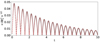 |
Fig. C.1 Decaying Alfvén wave test for |

References
- Adams, F. C., Hollenbach, D., Laughlin, G., & Gorti, U. 2004, ApJ, 611, 360 [NASA ADS] [CrossRef] [Google Scholar]
- Alcalá, J. M., Gangi, M., Biazzo, K., et al. 2021, A&A, 652, A72 [NASA ADS] [CrossRef] [EDP Sciences] [Google Scholar]
- Alexiades, V., Amiez, G., & Gremaud, P.-A. 1996, Commun. Numer. Methods Eng., 12, 31 [Google Scholar]
- Avenhaus, H., Quanz, S. P., Garufi, A., et al. 2018, ApJ, 863, 44 [NASA ADS] [CrossRef] [Google Scholar]
- Bai, X.-N. 2011, ApJ, 739, 50 [CrossRef] [Google Scholar]
- Bai, X.-N. 2013, ApJ, 772, 96 [Google Scholar]
- Bai, X.-N. 2017, ApJ, 845, 75 [NASA ADS] [CrossRef] [Google Scholar]
- Bai, X.-N., & Goodman, J. 2009, ApJ, 701, 737 [NASA ADS] [CrossRef] [Google Scholar]
- Bai, X.-N., & Stone, J. M. 2013, ApJ, 769, 76 [Google Scholar]
- Balbus, S. A.,& Hawley, J. F. 1991, ApJ, 376, 214 [Google Scholar]
- Benitez-Llambay, P., & Masset, F. S. 2016, ApJS, 223, 11 [NASA ADS] [CrossRef] [Google Scholar]
- Benitez-Llambay, P., Krapp, L., & Pessah, M. E. 2019, ApJS, 241, 25 [NASA ADS] [CrossRef] [Google Scholar]
- Béthune, W., Lesur, G., & Ferreira, J. 2017, A&A, 600, A75 [NASA ADS] [CrossRef] [EDP Sciences] [Google Scholar]
- Beuzit, J. L., Vigan, A., Mouillet, D., et al. 2019, A&A, 631, A155 [NASA ADS] [CrossRef] [EDP Sciences] [Google Scholar]
- Bjorkman, J. E., & Wood, K. 2001, ApJ, 554, 615 [NASA ADS] [CrossRef] [Google Scholar]
- Blaes, O. M., & Balbus, S. A. 1994, ApJ, 421, 163 [NASA ADS] [CrossRef] [Google Scholar]
- Blanco, D., Ricci, L., Flock, M., & Turner, N. 2021, ApJ, 920, 70 [NASA ADS] [CrossRef] [Google Scholar]
- Blandford, R. D., & Payne, D. G. 1982, MNRAS, 199, 883 [CrossRef] [Google Scholar]
- Brown, P. N., Byrne, G. D., & Hindmarsh, A. C. 1989, Siam J. Sci. Stat. Comput., 10, 1038 [CrossRef] [Google Scholar]
- Casse, F., & Keppens, R. 2002, ApJ, 581, 988 [Google Scholar]
- Chiang, E. I., & Goldreich, P. 1997, ApJ, 490, 368 [Google Scholar]
- Choi, E., Kim, J., & Wiita, P. J. 2009, ApJS, 181, 413 [NASA ADS] [CrossRef] [Google Scholar]
- Cui, C., & Bai, X.-N. 2021, MNRAS, 507, 1106 [NASA ADS] [CrossRef] [Google Scholar]
- Dominik, C., Min, M., & Tazaki, R. 2021, Astrophysics Source Code Library, [record ascl:2104.010] [Google Scholar]
- Draine, B. T., Roberge, W. G., & Dalgarno, A. 1983, ApJ, 264, 485 [CrossRef] [Google Scholar]
- Dubrulle, B., Morfill, G., & Sterzik, M. 1995, Icarus, 114, 237 [Google Scholar]
- Dullemond, C. P., & Dominik, C. 2004, A&A, 421, 1075 [NASA ADS] [CrossRef] [EDP Sciences] [Google Scholar]
- Dullemond, C. P., Juhasz, A., Pohl, A., et al. 2012, Astrophysics Source Code Library, [ascl:1202.015] [Google Scholar]
- Dzyurkevich, N., Flock, M., Turner, N. J., Klahr, H., & Henning, T. 2010, A&A, 515, A70 [NASA ADS] [CrossRef] [EDP Sciences] [Google Scholar]
- Dzyurkevich, N., Turner, N. J., Henning, T., & Kley, W. 2013, ApJ, 765, 114 [NASA ADS] [CrossRef] [Google Scholar]
- Ercolano, B., Drake, J. J., Raymond, J. C., & Clarke, C. C. 2008, ApJ, 688, 398 [Google Scholar]
- Ercolano, B., Clarke, C. J., & Drake, J. J. 2009, ApJ, 699, 1639 [Google Scholar]
- Ercolano, B., Picogna, G., Monsch, K., Drake, J. J., & Preibisch, T. 2021, MNRAS, 508, 1675 [NASA ADS] [CrossRef] [Google Scholar]
- Evans, C. R., & Hawley, J. F. 1988, ApJ, 332, 659 [Google Scholar]
- Fendt, C., & Sheikhnezami, S. 2013, ApJ, 774, 12 [Google Scholar]
- Ferreira, J., & Pelletier, G. 1993, A&A, 276, 625 [NASA ADS] [Google Scholar]
- Ferreira, J., & Pelletier, G. 1995, A&A, 295, 807 [NASA ADS] [Google Scholar]
- Flaherty, K. M., Hughes, A. M., Rosenfeld, K. A., et al. 2015, ApJ, 813, 99 [NASA ADS] [CrossRef] [Google Scholar]
- Flaherty, K. M., Hughes, A. M., Rose, S. C., et al. 2017, ApJ, 843, 150 [NASA ADS] [CrossRef] [Google Scholar]
- Flaischlen, S., Preibisch, T., Manara, C. F., & Ercolano, B. 2021, A&A, 648, A121 [NASA ADS] [CrossRef] [EDP Sciences] [Google Scholar]
- Flock, M., Dzyurkevich, N., Klahr, H., Turner, N. J., & Henning, T. 2011, ApJ, 735, 122 [NASA ADS] [CrossRef] [Google Scholar]
- Flock, M., Turner, N. J., Nelson, R. P., et al. 2020, ApJ, 897, 155 [Google Scholar]
- Font, A. S., McCarthy, I. G., Johnstone, D., & Ballantyne, D. R. 2004, ApJ, 607, 890 [NASA ADS] [CrossRef] [Google Scholar]
- Franz, R., Picogna, G., Ercolano, B., & Birnstiel, T. 2020, A&A, 635, A53 [EDP Sciences] [Google Scholar]
- Franz, R., Ercolano, B., Casassus, S., et al. 2022, A&A, 657, A69 [NASA ADS] [CrossRef] [EDP Sciences] [Google Scholar]
- Fromang, S., & Nelson, R. P. 2009, A&A, 496, 597 [NASA ADS] [CrossRef] [EDP Sciences] [Google Scholar]
- Fromang, S., & Papaloizou, J. 2007, A&A, 476, 1113 [NASA ADS] [CrossRef] [EDP Sciences] [Google Scholar]
- Fromang, S., Papaloizou, J., Lesur, G., & Heinemann, T. 2007, A&A, 476, 1123 [NASA ADS] [CrossRef] [EDP Sciences] [Google Scholar]
- Fromang, S., Latter, H., Lesur, G., & Ogilvie, G. I. 2013, A&A, 552, A71 [NASA ADS] [CrossRef] [EDP Sciences] [Google Scholar]
- Gammie, C. F. 1996, ApJ, 457, 355 [Google Scholar]
- Garufi, A., Podio, L., Bacciotti, F., et al. 2019, A&A, 628, A68 [NASA ADS] [CrossRef] [EDP Sciences] [Google Scholar]
- Getman, K. V., Flaccomio, E., Broos, P. S., et al. 2005, ApJS, 160, 319 [NASA ADS] [CrossRef] [Google Scholar]
- Giacalone, S., Teitler, S., Königl, A., Krijt, S., & Ciesla, F. J. 2019, ApJ, 882, 33 [NASA ADS] [CrossRef] [Google Scholar]
- Gombosi, T. I., Nagy, A. F., & Cravens, T. E. 1986, Rev. Geophys., 24, 667 [NASA ADS] [CrossRef] [Google Scholar]
- Gorti, U., & Hollenbach, D. 2009, ApJ, 690, 1539 [Google Scholar]
- Gressel, O., Turner, N. J., Nelson, R. P., & McNally, C. P. 2015, ApJ, 801, 84 [NASA ADS] [CrossRef] [Google Scholar]
- Gressel, O., Ramsey, J. P., Brinch, C., et al. 2020, ApJ, 896, 126 [Google Scholar]
- Haisch, K. E., Lada, E. A., & Lada, C. J. 2001, ApJ, 553, L153 [NASA ADS] [CrossRef] [Google Scholar]
- Hawley, J. F., & Stone, J. M. 1995, Comput. Phys. Commun., 89, 127 [NASA ADS] [CrossRef] [Google Scholar]
- Henyey, L. G., & Greenstein, J. L. 1941, ApJ, 93, 70 [Google Scholar]
- Hildebrand, R. H. 1983, QJRAS, 24, 267 [NASA ADS] [Google Scholar]
- Hollenbach, D., Johnstone, D., Lizano, S., & Shu, F. H. 1994, ApJ, 428, 654 [NASA ADS] [CrossRef] [Google Scholar]
- Hunter, J. D. 2007, Comput. Sci. Eng., 9, 90 [NASA ADS] [CrossRef] [Google Scholar]
- Hutchison, M. A., Laibe, G., & Maddison, S. T. 2016a, MNRAS, 463, 2725 [NASA ADS] [CrossRef] [Google Scholar]
- Hutchison, M. A., Price, D. J., Laibe, G., & Maddison, S. T. 2016b, MNRAS, 461, 742 [NASA ADS] [CrossRef] [Google Scholar]
- Igea, J., & Glassgold, A. E. 1999, ApJ, 518, 848 [Google Scholar]
- Ilgner, M., & Nelson, R. P. 2006, A&A, 445, 205 [CrossRef] [EDP Sciences] [Google Scholar]
- Klahr, H. H., & Bodenheimer, P. 2003, ApJ, 582, 869 [NASA ADS] [CrossRef] [Google Scholar]
- Klahr, H., & Hubbard, A. 2014, ApJ, 788, 788 [NASA ADS] [Google Scholar]
- Krapp, L., Gressel, O., Benítez-Llambay, P., et al. 2018, ApJ, 865, 105 [NASA ADS] [CrossRef] [Google Scholar]
- Lovelace, R. V. E., Li, H., Colgate, S. A., & Nelson, A. F. 1999, ApJ, 513, 805 [NASA ADS] [CrossRef] [Google Scholar]
- Lyra, W., Johansen, A., Zsom, A., Klahr, H., & Piskunov, N. 2009, A&A, 497, 869 [NASA ADS] [CrossRef] [EDP Sciences] [Google Scholar]
- Mamajek, E. E., Meyer, M. R., Hinz, P. M., et al. 2004, ApJ, 612, 496 [Google Scholar]
- Manger, N., & Klahr, H. 2018, MNRAS, 480, 2125 [NASA ADS] [CrossRef] [Google Scholar]
- Miyake, T., Suzuki, T. K., & Inutsuka, S.-i. 2016, ApJ, 821, 3 [Google Scholar]
- Nelson, R. P., Gressel, O., & Umurhan, O. M. 2013, MNRAS, 435, 2610 [Google Scholar]
- Okuzumi, S. 2009, ApJ, 698, 1122 [Google Scholar]
- Oppenheimer, M., & Dalgarno, A. 1974, ApJ, 192, 29 [NASA ADS] [CrossRef] [Google Scholar]
- Owen, J. E., & Kollmeier, J. A. 2019, MNRAS, 487, 3702 [Google Scholar]
- Owen, J. E., Ercolano, B., Clarke, C. J., & Alexander, R. D. 2010, MNRAS, 401, 1415 [Google Scholar]
- Owen, J. E., Ercolano, B., & Clarke, C. J. 2011, MNRAS, 411, 1104 [NASA ADS] [CrossRef] [Google Scholar]
- Owen, J. E., Clarke, C. J., & Ercolano, B. 2012, MNRAS, 422, 1880 [Google Scholar]
- Pfeil, T., & Klahr, H. 2021, ApJ, 915, 130 [NASA ADS] [CrossRef] [Google Scholar]
- Picogna,G., Ercolano, B., Owen, J. E., & Weber, M. L. 2019, MNRAS, 487, 691 [NASA ADS] [CrossRef] [Google Scholar]
- Picogna, G., Ercolano, B., & Espaillat, C. C. 2021, MNRAS, 508, 3611 [NASA ADS] [CrossRef] [Google Scholar]
- Pollack, J. B., Hollenbach, D., Beckwith, S., et al. 1994, ApJ, 421, 615 [Google Scholar]
- Ribas, Á., Bouy, H., & Merín, B. 2015, A&A, 576, A52 [NASA ADS] [CrossRef] [EDP Sciences] [Google Scholar]
- Riols, A., & Lesur, G. 2018, A&A, 617, A117 [NASA ADS] [CrossRef] [EDP Sciences] [Google Scholar]
- Rodenkirch, P. J., Klahr, H., Fendt, C., & Dullemond, C. P. 2020, A&A, 633, A21 [NASA ADS] [CrossRef] [EDP Sciences] [Google Scholar]
- Shakura, N. I., & Sunyaev, R. A. 1973, A&A, 500, 33 [NASA ADS] [Google Scholar]
- Sheikhnezami, S., Fendt, C., Porth, O., Vaidya, B., & Ghanbari, J. 2012, ApJ, 757, 65 [NASA ADS] [CrossRef] [Google Scholar]
- Stammler, S. M., & Dullemond, C. P. 2014, Icarus, 242, 1 [NASA ADS] [CrossRef] [Google Scholar]
- Stepanovs, D., & Fendt, C. 2014, ApJ, 793, 31 [NASA ADS] [CrossRef] [Google Scholar]
- Stepanovs, D., & Fendt, C. 2016, ApJ, 825, 14 [Google Scholar]
- Stoll, M. H. R., & Kley, W. 2014, A&A, 572, A77 [NASA ADS] [CrossRef] [EDP Sciences] [Google Scholar]
- Stoll, M. H. R., & Kley, W. 2016, A&A, 594, A57 [NASA ADS] [CrossRef] [EDP Sciences] [Google Scholar]
- Suriano, S. S., Li, Z.-Y., Krasnopolsky, R., & Shang, H. 2018, MNRAS, 477, 1239 [NASA ADS] [CrossRef] [Google Scholar]
- Suzuki, T. K., & Inutsuka, S. I. 2009, ApJ, 691, L49 [NASA ADS] [CrossRef] [Google Scholar]
- Suzuki, T. K., Muto, T., & Inutsuka, S.-i. 2010, ApJ, 718, 1289 [NASA ADS] [CrossRef] [Google Scholar]
- Tzeferacos, P., Ferrari, A., Mignone, A., et al. 2009, MNRAS, 400, 820 [NASA ADS] [CrossRef] [Google Scholar]
- Umebayashi, T., & Nakano, T. 2009, ApJ, 690, 69 [Google Scholar]
- Ustyugova, G. V., Koldoba, A. V., Romanova, M. M., Chechetkin, V. M., & Lovelace, R. V. E. 1999, ApJ, 516, 221 [NASA ADS] [CrossRef] [Google Scholar]
- Wang, L., Bai, X.-N., & Goodman, J. 2019, ApJ, 874, 90 [Google Scholar]
- Wardle, M., & Koenigl, A. 1993, ApJ, 410, 218 [Google Scholar]
- Weber, P., Pérez, S., Benítez-Llambay, P., et al. 2019, ApJ, 884, 178 [NASA ADS] [CrossRef] [Google Scholar]
- Woitke, P., Min, M., Pinte, C., et al. 2016, A&A, 586, A103 [NASA ADS] [CrossRef] [EDP Sciences] [Google Scholar]
- Youdin, A. N., & Lithwick, Y. 2007, Icarus, 192, 588 [NASA ADS] [CrossRef] [Google Scholar]
- Zanni, C., Ferrari, A., Rosner, R., Bodo, G., & Massaglia, S. 2007, A&A, 828, 20 [Google Scholar]
All Tables
All Figures
|
Fig. 1 Gas density maps of the simulations phc2, b5c2 and b4c2 after 500 orbits at 1 au. Magnetic field lines are represented by the white lines in the corresponding panels. The color map scaled logarithmically annotated by the exponent to a base of ten and represents the volume density of the gas in g cm−3. |
| In the text | |
|
Fig. 2 Total wind mass loss rates of gas and dust for the simulation runs phc2, b5c2, b4c2 and b4c2np. Results from 10 μm grains are excluded due to the negligible outflow and the lack of entrainment in the wind for all runs shown above. |
| In the text | |
|
Fig. 3 Dust density maps for the simulations phc2, b5c2 and b4c2 after 500 orbits at 1 au. Dust velocity streamlines are annotated by the white arrowed lines. The upper, center and lower three panels visualize the flow of grains with size 0.1 μm, 1 μm and 10 μm, respectively. |
| In the text | |
|
Fig. 4 Dust density maps for the simulation b4c2np after 500 orbits at 1 au. Dust velocity streamlines are annotated by the white arrowed lines. |
| In the text | |
|
Fig. 5 Cumulative mass loss rates of gas and dust for the simulation runs phc2, b5c2, b4c2 and b4c2a3 starting from 3 au. The cylindrical radius or foot point of the loss is obtained by tracing backwards the corresponding streamline from the outer radial boundary down to 5 scale heights above the disk mid plane. The flow field is averaged over 50 orbits at 1 au starting at 600 orbits. The vertical dashed lines mark the limit of the region where 99% of the mass loss occurred. |
| In the text | |
|
Fig. 6 Numerically integrated dust trajectories for snapshots after 500 T0 of the simulation runs phc2, b5c2 and b4c2. The orange color map represents the gas density and the thin arrowed white lines denote the gas velocity streamlines. The thicker colored lines visualize the dust trajectories for grain sizes ranging from 0.1 μm to 10 μm. |
| In the text | |
|
Fig. 7 Asymptotic dust flow inclination depending on the grain size for the simulation runs phc2, b5c2, b4c2 and b4c2np. |
| In the text | |
|
Fig. 8 Normalized vertical density slices of the phc2 at different radial locations in the disk. The violet lines represent the normalized gas density while the turquoise lines display the dust density of 10 μm grains. The gray lines denote the respective Stokes number profile. |
| In the text | |
|
Fig. 9 Normalized vertical density slices and Stokes number profiles of the phc2 similar to Fig. 8 for the grain sizes 0.1 μm (straight lines), 1 μm (dashed lines), 10 μm (dotted lines) at 5 au. |
| In the text | |
|
Fig. 10 Physical quantities at the wind launching surface of the simulation runs phc2 (straight lines), b5c2 (dashed lines) and b4c2 (dotted lines). In the top two panels the blue lines represent 0.1 μm -sized grains, whereas the green lines denote 1 μm-sized grains. |
| In the text | |
|
Fig. 11 Streamlines starting from r = 8 au, z = 2.5 au. Shown are poloidal velocities of gas and dust along the streamline (left two panels) and the respective Stokes numbers St as well as the Alfvén Mach number MA (right two panels). |
| In the text | |
|
Fig. 12 H-band radial optical depth τobs originating from the central star depending on the inclination expressed in latitude for three dust species with sizes 0.1 μm, 1 μm and 10 μm indicated by the color scheme. The continuous lines refer to the photoevaporation simulation phc2, the dashed lines to the magnetic wind b5c2 with β = 105 and the dotted lines to the run b4c2 with β = 104. |
| In the text | |
|
Fig. 13 Radiative transfer images in the H-band (λ = 1.6 μm) of simulation runs with photoevaporation (left most column), β = 105 (center left column), β = 104 (center right column) and a cold magnetic wind with β = 104 (right most column). The upper panels are based on dust grains with a = 0.1 μm whereas the lower panels demonstrate synthetic images with a = 1 μm. The object is modeled at a distance of 150 pc with a solar type star at an inclination of 20°. |
| In the text | |
|
Fig. 14 Radiative transfer images in the H-band (λ = 1.6 μm) of the same simulation runs as in Fig. 13 but with an edge-on view at an inclination of 0°. |
| In the text | |
|
Fig. A.1 Vertical slices of gas and dust temperatures at different radial location in the disk and wind region of the photoevaporation simulation phc2. The gray lines represent the gas temperatures whereas the red lines display the equilibrium dust temperatures of the 0.1 μm grains. |
| In the text | |
|
Fig. B.1 Normalized dust density (blue lines) and ionization fraction (gray lines) in the simulations b4c2 and b4c2eps2 with a dust-to-gas ratio of ϵ = 10−3 and ϵ =10−2, respectively. The snapshot is taken after 1000 orbits at 1 au. |
| In the text | |
|
Fig. C.1 Decaying Alfvén wave test for |
| In the text | |
 |
Fig. C.2 Decaying Alfvén wave test for |
| In the text | |
Current usage metrics show cumulative count of Article Views (full-text article views including HTML views, PDF and ePub downloads, according to the available data) and Abstracts Views on Vision4Press platform.
Data correspond to usage on the plateform after 2015. The current usage metrics is available 48-96 hours after online publication and is updated daily on week days.
Initial download of the metrics may take a while.