| Issue |
A&A
Volume 659, March 2022
|
|
|---|---|---|
| Article Number | A37 | |
| Number of page(s) | 14 | |
| Section | Interstellar and circumstellar matter | |
| DOI | https://doi.org/10.1051/0004-6361/202141997 | |
| Published online | 01 March 2022 | |
Photometric signatures of corotating magnetospheres of hot stars governed by higher-order magnetic multipoles
1
Department of Theoretical Physics and Astrophysics, Masaryk University,
Kotlářská 2,
61137
Brno,
Czech Republic
e-mail: This email address is being protected from spambots. You need JavaScript enabled to view it.
2
Department of Physics, California Lutheran University,
60 West Olsen Road #3700,
Thousand Oaks,
CA
91360, USA
3
LESIA, Paris Observatory, PSL University, CNRS, Sorbonne University, Univ. Paris Diderot, Sorbonne Paris Cité,
5 place Jules Janssen,
92195
Meudon, France
Received:
10
August
2021
Accepted:
21
January
2022
Abstract
Context. The light curves of magnetic, chemically peculiar stars typically show periodic variability due to surface spots that in most cases can be modeled by low-order harmonic expansion. However, high-precision satellite photometry reveals tiny complex features in the light curves of some of these stars that are difficult to explain as caused by a surface phenomenon under reasonable assumptions. These features might originate from light extinction in corotating magnetospheric clouds supported by a complex magnetic field dominated by higher-order multipoles.
Aims. We aim to understand the photometric signatures of corotating magnetospheres that are governed by higher-order multipoles.
Methods. We determined the location of magnetospheric clouds from the minima of the effective potential along the magnetic field lines for different orders of multipoles and their combination. From the derived magnetospheric density distribution, we calculated light curves accounting for absorption and subsequent emission of light.
Results. For axisymmetric multipoles, the rigidly rotating magnetosphere model is able to explain the observed tiny features in the light curves only when the higher-order multipoles dominate the magnetic field not only at the stellar surface, but even at the Kepler radius. However, even a relatively weak nonaxisymmetric component leads to warping of equilibrium surfaces. This introduces structures that can explain the tiny features observed in the light curves of chemically peculiar stars. The light emission contributes to the light variability only if a significant fraction of light is absorbed in the magnetosphere.
Key words: stars: magnetic field / stars: chemically peculiar / stars: early-type / circumstellar matter / stars: variables: general
© ESO 2022
1 Introduction
Classical chemically peculiar stars are stars in the upper part of the main sequence, where the diffusion due to competing radiative and gravitational forces leads to chemical peculiarity (Michaud 1970; Vauclair et al. 1991; Vick et al. 2011). In chemically peculiar stars, the elements concentrate in vast surface spots (patches), which are formed by the influence of the magnetic field (Alecian & Stift 2017) and likely also by other processes (Kochukhov & Ryabchikova 2018; Jagelka et al. 2019). As a result of rotational modulation, the spots cause periodic spectroscopic and photometric variability.
Unlike the spots on cool stars, the patches on chemically peculiar stars are mostly stable over at least decades (e.g., Adelman 2006; Mikulášek et al. 2008) and have the same effective temperature as the rest of the surface. The latter follows from the fact that most of the light variability of these stars can be explained as a result of flux redistribution due to bound-free (Peterson 1970; Krtička et al. 2007) and bound-bound transitions (Wolff & Wolff 1971; Molnar 1973; Krtička et al. 2009; Shulyak et al. 2010; Prvák et al. 2015) of helium and heavier elements such as silicon, chromium, and iron.
It is commonly assumed that as a result of their modulation by rotation, light curves of chemically peculiar stars can be typically reproduced using low-order harmonic expansion (e.g., Mikulášek et al. 2007; Shultz et al. 2019a). However, high-precision satellite photometry changed this picture. In addition to the variability that can be attributed to spots, a large fraction of hot chemically peculiar stars (Mikulášek et al., in prep.) shows tiny complex features (also known as warps) on their light curves (Hümmerich et al. 2018; Mikulášek et al. 2020). These narrow features in the light curves do not appear on theoretically simulated light curves of chemically peculiar stars (e.g., Krtička et al. 2009; Shulyak et al. 2010). Moreover, narrow features are difficult to explain by surface modulation under reasonable assumptions about the intensity contrast of spots and their sharpness (Prvák 2019, Sects. 5.3 and 5.5).
On the other hand, the rotational light variability of chemically peculiar stars can be caused by sources other than surface patches. A large fraction of chemically peculiar stars may have winds driven by the line radiative force (Abbott 1979; Babel 1996; Krtička 2014). Even below the limit of hydrogen-dominated winds, however, purely metallic winds are possible (Babel 1995). Within the rigidly rotating magnetosphere model, the stellar wind flows along magnetic field lines and accumulates in the region of minimum effective potential given by centrifugal and gravitational forces. The magnetospheric clouds established by this process occult part of the stellar surface, which may lead to dips (eclipses) in the light curve (Landstreet & Borra 1978; Nakajima 1985; Smith & Groote 2001; Townsend et al. 2005). Only a few stars show dips on their light curves in ground-based observations (e.g., Townsend et al. 2005; Oksala et al. 2010; Grunhut et al. 2012). On the other hand, many more such stars may be detected with high-precision satellite photometry, which can be connected with the absorption of stellar radiation by corotating magnetospheric clouds.
In principle, the observed tiny features in the light curves can be also interpreted in terms of additional emission (bumps) instead of absorption. However, the width of these features would imply a strong beaming of the radiation, which might be less conceivable than simple absorption by intervening clouds.
The accumulation of matter in dipolar field with a high obliquity leads to two isolated minima in the light curve (Townsend et al. 2005). Therefore, a magnetic field dominated by higher-order multipoles might explain the light curves with numerous warps. A similar model was proposed by Jardine et al. (2001) to provide prominence support in the magnetospheres of cool stars. We examine this possibility in this paper, which is organized as follows. Section 2 gives the structure of equilibrium surfaces at which the magnetospheric matter accumulatesfor a magnetic field dominated by higher-order multipoles, while Sect. 3 predicts the light curves induced by these magnetospheres. Finally, in Sect. 4 we discuss an application of our model to typical chemically peculiar stars with warped light curves, and Sect. 6 presents our conclusions.
2 Rotating magnetosphere model for general multipoles
A physically motivated distribution of the matter in the magnetosphere of a rotating star can be obtained by elaborating the models proposed byPreuss et al. (2004) and Townsend & Owocki (2005). The latter model is more general and allows determining the density distribution accounting for the wind mass-loss rate modulation due to the magnetic field. The model was successfully applied not only to study the light curves due to circumstellar absorption, but also to provide a detailed interpretation of Hα magnetospheric emission (e.g., Oksala et al. 2015; Shultz et al. 2020) and polarimetry (Carciofi et al. 2013).
In a corotating circumstellar magnetosphere, the ionized matter is at rest when the sum of the gravitational and centrifugal force (per unit of mass) f is perpendicular to the magnetic field,
 (1)
(1)
where
![Mathematical equation: \begin{equation*}\boldsymbol{f}=\boldsymbol{g}-\boldsymbol{\Omega}\times \left(\boldsymbol{\Omega}\times\boldsymbol{r}\right)= \frac{GM}{r_{\textrm{K}}^2}\left[\boldsymbol{\xi}\left(1-\frac{1}{\xi^3}\right)- \boldsymbol{\omega}\left(\boldsymbol{\omega}\cdot\boldsymbol{\xi}\right)\right], \end{equation*}](/articles/aa/full_html/2022/03/aa41997-21/aa41997-21-eq2.png) (2)
(2)
and g stands for gravity acceleration, Ω = Ωω is the angular frequency, b = B∕B is the unit vector in the direction of magnetic field B, and ξ = r∕rK is the radius vector r in units of the Kepler radius,
 (3)
(3)
The stability condition further requires that the displacement of an element from the equilibrium position along the field line b leads to the appearance of the force in the opposite direction, that is,
 (4)
(4)
In the model of Townsend & Owocki (2005), this corresponds to the potential minimum along the field line. Inserting the effective force in Eq. (2), the stability condition Eq. (4) can be rewritten as
![Mathematical equation: \begin{equation*}\frac{1}{\xi^3}\left[\frac{3}{\xi^2}\left(\boldsymbol{b}\cdot\boldsymbol{\xi}\right)^2-1\right]+ 1-\left(\boldsymbol{\omega}\cdot\boldsymbol{b}\right)^2+ \boldsymbol{f}_{\xi} \cdot\left(\boldsymbol{b}\nabla_{\xi}\right)\boldsymbol{b}<0. \end{equation*}](/articles/aa/full_html/2022/03/aa41997-21/aa41997-21-eq5.png) (5)
(5)
Here ∇ξ denotes the gradient in nondimensional units, ∇ξ = rK∇ and  .
.
2.1 Field aligned with rotational axis
In the simplest case, the axes of the multipole and the rotational axis are parallel. The magnetic field strength is modeled using co-aligned axisymmetric multipoles of the order n,
 (6)
(6)
where Pn and  denote the Legendre and associated Legendre polynomials, respectively. We do not account for a field with a nonzero azimuthal component in the initial calculations. The plots of the equilibrium surfaces Eq. (1) fulfilling the stability condition Eq. (4) are given in Fig. 1.
For a dipolar case (n = 1), the resulting equilibrium surface corresponds to an equatorial plane with a hole. In the equatorial plane, the force f is perpendicular to the magnetic field fulfilling the equilibrium condition of Eq. (1). The central hole appears from the stability condition Eq. (4). For a dipolar field in the equatorial plane, b ⋅ ξ = 0 and ω ⋅ b = 1, and after an evaluation of the gradient term, the stability condition consequently is (Preuss et al. 2004; Townsend & Owocki 2005)
 (7)
(7)
Therefore, as a result of the influence of the magnetic field, the matter is stable even slightly below the Kepler radius ξ = 1.
There are additional equilibrium chimney-like surfaces in the polar direction (Preuss et al. 2004), where the force f is perpendicular to the magnetic field. However, the equilibrium on these surfaces is unstable because either gravity or centrifugal force drives the matter out of the equilibrium position.
The quadrupole (n = 2) has two lobes below and above the equatorial plane, therefore there are two surfaces at which the matter is in equilibrium and is stable (Fig. 1; see also Jardine et al. 2001). In general, there is an equilibrium surface for each lobe of the multipole. The apex of the lobe appears where the radial component of the magnetic field is zero, which from Eq. (6) corresponds to the root of the appropriate Legendre polynomial. The number of roots is given by an order of multipole, therefore the number of lobes is equal to the order of the multipole. The surfaces show a mirror symmetry with respect to the equatorial plane, and this plane consequently corresponds to stable solutions for odd multipoles. At large distances from the star, the effective force in the equilibrium condition f ⋅ b = 0 is dominated by the centrifugal force, which is perpendicular to the rotational axis. Therefore, the equilibrium condition is fulfilled at the surface where the magnetic field is parallel to the rotational axis. Individual magnetic field lines are similar, therefore the magnetic field is parallel to the rotational axis for a particular θ. As a result, at large distances from the star, the equilibrium surfaces is conical.
This also explains why there is one equilibrium surface for each order of the multipole. The order of multipole determines the number of lobes. In each lobe, there is just one magnetic latitude where the magnetic field lines are perpendicular to the effective force, therefore there is just one equilibrium surface per each lobe or multipolar order. In the equatorial plane, the effective force is radial, therefore the equilibrium surface appears at the apex of the lobe where the radial magnetic field component is zero. This is given by the root of the corresponding Legendre polynomial. Outside the equatorial plane, the effective force is no longer radial, therefore the equilibrium surface does not appear at the apex of the lobe.
For odd multipoles, one of the equilibrium surfaces always appears in the equatorial plane. Taking into account Eq. (2), the stability condition Eq. (5) simplifies to − 1∕ξ3 + γ(1 − 1∕ξ3) < 0, where  . Evaluating the directional derivative in the equatorial plane in spherical coordinates taking into account the properties of the Legendre polynomials and Eq. (6) gives γ = −n − 2. Therefore, the solution of the inequality leads to a generalized condition of Eq. (7),
 (8)
(8)
This means that with an increasing order of the multipole, the radius of the central hole grows from  (Eq. (7)) to ξ = 1. This corresponds to a change in equilibrium condition with the variation of the order of the multipole. For a uniform magnetic field parallel with the rotational axis, the matter would be stable anywhere in the equatorial plane. With increasing order of the multipole, the magnetic field lines become increasingly bended. Therefore, for multipoles with high order, the matter becomes stable if the centrifugal force is stronger than gravity, as is usually the case without a magnetic field, and the radius of the central hole approaches ξ = 1. The numerical results show that below and above the equatorial plane, the matter is stable outside the cylinder with radius ξ ≈ 1.
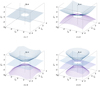 |
Fig. 1 Equilibrium surfaces Eq. (1) fulfilling the stability condition Eq. (4) for a field aligned with the stellar rotational axis and multipoles with different orders. |
2.2 Misaligned rotation
The axis of the magnetic field is typically tilted with respect to the rotational axis in magnetic, hot stars. We denote the angle between these axes (the magnetic field obliquity) by β. For β > 0, the equilibrium surfaces become warped, as we show in Fig. 2. As in aligned case, there is one equilibrium surface per multipole order. In addition, part of the chimney-like surface that was unstable for a field aligned with the rotational axis becomes stable because potential minima appear at the surface.
In the case of misaligned rotation, the axis of the cylinder oriented along the rotational axis with radius ξ = 1, outside of which the stability condition is fulfilled, is tilted with respect to the magnetic axis. As a result, the region closest to the star where the matter is in stable equilibrium, appears at the intersection of the magnetic and rotational equators (Townsend & Owocki 2005).
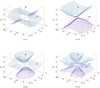 |
Fig. 2 Equilibrium surfaces Eq. (1) fulfilling the stability condition Eq. (4) for a rotational axis ω tilted by 5∕12 π with respect to the axis of the magnetic field b for multipoles with different orders. Both axes are denoted in the graph. |
2.3 General combination of coaligned multipoles
The structure of the magnetic field of a hot star is typically not given by just one multipole, but is much more complex (e.g., Kochukhov et al. 2011; Rusomarov et al. 2015; Silvester et al. 2017). Therefore, we have to combine multipoles with different orders to understand the formation of the equilibrium surfaces in more realistic situations. In Fig. 3 we provide plots of individual equilibrium surfaces for different ratios of Bm ∕Bn at the Keplerian radius ξ = 1 and for different orders m and n (m >n), assuming that the multipoles share the axis of symmetry.
From Fig. 3 it follows that the equilibrium surfaces are dominated by lower-order multipoles for Bm ≲ Bn. The presence of additional multipoles is manifested by a slight shift of the equilibrium surface for the case of multipoles with different parity. As the amplitude of the higher-order multipole increases, a new equilibrium surface appears, which in the limit Bm ≫ Bn approaches the structure of surfaces corresponding to the order m (cf. Fig. 1). The new surface(s) has a toroidal shape for multipoles of the same parity or a cone-like shape for multipoles with different parity.
Figure 4 explains why the lower multipole order dominates even for Bm ≈ Bn. Here we plot the magnetic strength vector for the dipolar and quadrupolar component in the y = 0 plane. The strength of the dipolar component is always normalized to unity, while the quadrupolar component is plotted relative to the dipolar component, that is, with the length reduced by a factor of 1∕ξ. The total magnetic field strength is given by the sum of these components. The figure shows that the quadrupolar component changes the orientation of the dominating dipole component only slightly in most cases. This results in a warping of the equilibrium surface, but no new equilibrium surface appears. Additional surfaces appear only when the quadrupolar surface dominates the whole region.
These simulations show that a complexly warped light curve may appear only in stars in which the higher-order multipole dominates even at the Keplerian radius ξ = 1. Because magnetic field components corresponding to higher-order multipoles decrease fast, this implies an even stronger dominance at the stellar radius. This condition can be partly mitigated by fast rotation, in which case the stellar radius is close to the Keplerian radius.
 |
Fig. 3 Equilibrium surfaces fulfilling the stability condition for a field aligned with the rotational axis and a combination of multipoles with different orders. |
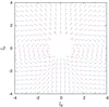 |
Fig. 4 Magnetic field vector for the dipolar (blue) and quadrupolar (red) field plotted in the y = 0 plane. The dipolar component is plotted with the unit length vector, and the length of the quadrupolar field vector is reduced by afactor of 1∕ξ. |
2.4 Nonaxisymmetric multipoles
We have considered only axisymmetric multipoles so far. However, the general multipole expansion also accounts for nonaxisymmetric terms (e.g., Jardine et al. 1999). To understand their effect, we accounted for the multipolar expansion in the form of
 (9)
(9)
The nonaxisymmetric terms do not affect the shape of the equilibrium surface when the field is aligned with the rotational axis because the sum of the gravitational and centrifugal force f has a zero azimuthal component, and the radial and longitudinal field components both depend on ϕ in the same way. As a result, the condition described by Eq. (1) is not affected, and the equilibrium surfaces are given by the radial and latitudinal components of the magnetic field. The numerical analysis shows that the equilibrium surfaces resemble those for multipolar fields given in Fig. 1.
Because the individual magnetic field components depend on the radius in the same way, the magnetic field lines are similar in the nonaxisymmetric case as well. Therefore, the equilibrium surface takes a conical shape in the limit of large ξ for the same reasons as in the axisymmetric case. From a similar analytical analysis as in Sect. 2.1 it follows that the radius of the central hole that appears in the equatorial plane from stability considerations is not affected by the azimuthal magnetic field and is given by Eq. (8).
Because the number of lobes is given by the number of roots of the radial component of the magnetic field, the number of equilibrium surfaces given by the numbers of lobes could be higher than in the axisymmetric case. For instance, for l = 1, there is one additional root of the associated Legendre polynomial, therefore the number of equilibrium surfaces is n + 1. These surfaces show a mirror symmetry, therefore for a field that is aligned with the rotational axis, the equatorial surface fulfills the equilibrium condition for even n.
At the apex of individual lobes where  , only the latitudinal magnetic field component remains. This component is modulated by a factor of cos (lϕ), which has 2l roots. Therefore, there are 2l directions ineach lobe where the flow can move freely and escape the star. In reality, this picture may be modified by other field components. Because the effective acceleration is not radial above the equatorial plane, the apex of each lobe does not coincide with the equilibrium surface, as in the axisymmetric case.
For cos(lϕ) = 0, only the azimuthal component of the magnetic field is nonzero; consequently, f ⋅ b = 0 for aligned rotational and magnetic axes, and new equilibrium surfaces appear. These surfaces are planes with a common line of intersection corresponding to the magnetic axis. The stability condition Eq. (5) for a particular case of a nonaxisymmetric multipole as in Eq. (9) can after some manipulation be rewritten as
 (10)
(10)
For instance, in the equatorial plane cosθ = 0, this gives the condition ξ > 1, that is, the equilibrium is stable above the Keplerian radius. In the general case, the plane is stable for large ξ. The numerical analysis has shown that Eq. (10) allows a stable equilibrium even below the Keplerian radius for ξ < 1. With increasing complexity of the field (for higher n), the smallest radius for which Eq. (10) is satisfied moves toward the star, but it can never reach zero (as show below).
The stability condition has a particularly illuminating form for a purely radial force (with fr (r)< 0) when the magnetic field is governed by a single component. For radial force fields, the equilibrium condition Eq. (1) requires that the radial component of the magnetic field unit vector is zero, br = 0. This is fulfilled in the apex of magnetic lobes corresponding to the roots of the Legendre polynomials  (see Eq. (9)). Because at the apex of the lobes, the longitudinal magnetic field component is zero as well, bϕ = 0, the stability condition Eq. (4) simplifies to
 (11)
(11)
Inserting the multipolar field Eq. (9) and canceling the positive terms, this can be rewritten as
 (12)
(12)
which is never fulfilled. Therefore, the stability in the case of a centered magnetic field governed by a single component always requires the presence of centrifugal force. A similar condition can be derived also for cos (lϕ) = 0 surfaces. For a general field, which can be described by a combination of several components, the stability condition reads
 (13)
(13)
Using the zero current condition rot(Bb) = 0, this can be rewritten as
 (14)
(14)
This is difficult to fulfill for any radially decreasing magnetic field. Therefore, either a centrifugal force or possibly nonzero currents are required for stability.
The field strength of the nonaxisymmetric multipoles varies with the same power of radius as the strength of the axisymmetric multipoles. Therefore, low-order multipoles dominate the magnetic field even in the nonaxisymmetric case unless the expansion coefficients in Eq. (9) are sufficiently high. However, the magnetic field component in the direction of force is zero around the equilibrium surfaces. Consequently, even a small additional magnetic field may dominate here and perturb the equilibrium surface. This is shown in Fig. 5 (lower panel), where we plot the equilibrium surface for the combination of the axisymmetric dipole and nonaxisymmetric octupole with l = 3. For a dipole, the equilibrium surface appears in the equatorial plane and corresponds to the apex of the lobe of the magnetic field, where the radial field component is zero. Consequently, even a relatively weak non-axisymmetric octupole that lacks the apex of the lobe in the equatorial plane is able to warp the equilibrium plane. Here the number of warps is equal to l = 3.
Equilibrium surfaces become warped only if the surfaces of individual multipoles do not coincide. In the opposite case, the splitting of surfaces may appear as a result of the interaction of nearby equilibrium surfaces (see Fig. 5 for l = 2 case). Relatively complex shapes of the equilibrium surfaces can also be derived from a combination of multipoles with the same order, but with different l.
2.5 Radius of the magnetosphere
The magnetic field dominates the magnetosphere up to the Alfvén radius RA, at which the magnetic field energy density is equal to the stellar wind kinetic energy density (ud-Doula & Owocki 2002). Therefore, the Alfvén radius can be derived from the condition
 (15)
(15)
For multipolar magnetic field  and stellar wind density given by ρ = Ṁ∕(4πr2v∞), at large distance from the star (v = v∞), the Alfvén radius is
 (16)
(16)
where
 (17)
(17)
which is the wind magnetic confinement parameter (ud-Doula & Owocki 2002). A strong dependence of the Alfvén radius on the order of the multipole means that even in the case of a very high magnetic field confinement η* ≈ 105−107 (Shultz et al. 2019b), the Alfvén radius is just a few times higher than the stellar radius for n > 3. In this case, the Alfvén radius may become smaller than the Kepler radius, preventing the existence of stable magnetospheric matter.
When the velocity is dominated by the rotational velocity, the condition Eq. (15) should be modified to (Trigilio et al. 2004)
 (18)
(18)
For solid-body rotation, vrot(r) = vrot(R*)r∕R*, and using the stellar wind density, the Alfvén radius is given by
 (19)
(19)
Because the ratio of the terminal wind speed and the equatorial rotational velocity typically is a factor of a few (Castor et al. 1975), depending on the stellar parameters, Eq. (19) could give an even smaller Alfvén radius than Eq. (16). For higher-order multipoles, both expressions give results close to the stellar radius.
Above the Alfvén radius, the magnetic field no longer dominates and the wind flows nearly radially (ud-Doula & Owocki 2002). The region of equipartition between the magnetic field energy density and the wind energy density around the Alfvén radius is the region of the reconnection events. They may accelerate particles to relativistic energies (Trigilio et al. 2004; Leto et al. 2006).
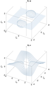 |
Fig. 5 Equilibrium surface fulfilling the stability condition for a field aligned with the rotational axis and combination of the axisymmetric dipole and octupole with l = 2 (upper panel) and l = 3 (lower panel). Plotted for B3,2∕B1 = 0.3 or B3,3 ∕B1 = 0.3. |
3 Light curves due to a rotating magnetosphere
The matter accumulates on equilibrium surfaces in the region of stability (Townsend & Owocki 2005). The density is highest in the part of the surface that is closest to the star. This material may obstruct the radiation emitted by the star and obscure part of the stellar surface. Wind models (Krtička 2014) show that absorption is most likely dominated by the light scattering on free electrons. The obscuration is highest for rays that are tangential to the equilibrium surface, because these rays encounter the largest amount of the material. As the star rotates, different parts of the equilibrium surface obstruct the line of sight. Therefore, the obscuration depends on the rotational phase and the light curve displays eclipses, as shown in Townsend et al. (2005).
The analysis of high-precision satellite photometry revealed that some chemically peculiar stars display small dips on their light curves.These features look like absorption features and typically do not come in isolation, but (when present) up to a dozen or more of such features appear in the light curve (Mikulášek et al. 2020). In our model, the number of these features per rotational period increases with the complexity of the field, therefore with the order of the multipole. From this, it seems that the warped light curves of chemically peculiar stars can be explained by the light absorption in corotating clouds that are trapped by the magnetic field that is described by multipoles of high order.
The magnetospheric matter settles in the magnetosphere, and its density distribution is given by the hydrostatic equilibrium along each field line (Townsend & Owocki 2005),
![Mathematical equation: \begin{equation*}\rho(\Delta s)=\rho_{\textrm{m}}\exp\left[-\frac{\mu\Delta\Phi(\Delta s)}{kT}\right], \end{equation*}](/articles/aa/full_html/2022/03/aa41997-21/aa41997-21-eq27.png) (20)
(20)
where ΔΦ(Δs) is the difference between the potential at a given point and the potential minimum located at the distance Δs along the field line, ρm is the matter density at the potential minimum, μ is the mean molecular weight, and k is the Boltzmann constant. Approximating ΔΦ by its Taylor expansion and using Eq. (4), ΔΦ(Δs) ≈−f′Δs2∕2. Therefore, the density distribution Eq. (20) takes the form of
 (21)
(21)
with the square of the characteristic scale height,
 (22)
(22)
The density ρm is different for individual field lines, and Townsend & Owocki (2005) accounted for stellar wind feeding to determine its value. However, the observational characteristics of Hα line profiles (Shultz et al. 2020) show that the magnetospheric matter density is given by a complex interplay between wind feeding and gas leakage either via diffusion and drift (Owocki & Cranmer 2018) or more likely by centrifugal breakout (Owocki et al. 2020). Consequently, we simply assumed ρm = Aξ−6 (Owocki et al. 2020), where A determines the total amount of mass in the magnetosphere.
3.1 Light absorption due to the circumstellar magnetosphere
As the circumstellar matter obstructs the rays aimed at a distant observer, it absorbs the stellar radiation and causes the light variability. The intensity along the ray is reduced according to
 (23)
(23)
where the optical depth is given by
 (24)
(24)
where we used Eq. (21), l denotes the length variable along the ray, mH is the hydrogen mass, and σT is the Thompson scattering cross-section. We integrated the specific intensity from Eq. (23) across the visible stellar surface for different viewing angles to obtain the phase-dependent light curve.
The magnetospheric matter accumulates around the equilibrium surfaces Eq. (1). For an axisymmetric magnetic field with β =0, the resulting density distribution is also axisymmetric. Consequently, there is no rotational variability in the case of aligned rotation of axisymmetric multipoles. For β > 0, the equilibrium surfaces become warped even for the case of multipoles that are axially symmetric around the magnetic axis. Most of the matter accumulates in the surface regions closest to the star, leading to a modulation of the light variability by the rotation.
Figure 6 shows light curves for different combinations of multipoles. We adopted a stellar mass M = 8 M⊙, a radius R = 4 R⊙, and a rotation period P = 1 d roughly corresponding to σ Ori E (Oksala et al. 2015). The light curves are plotted for a magnetic axis perpendicular to the rotational axis (β = π∕2) and for an equator-on orientation (i = π∕2). This gives the largest amplitude of the variability (Townsend 2008). With a nonzero magnetic axis tilt, the equilibrium surfaces become warped with the maximum density of matter in the surface regions closest to the star. As the equilibrium surfaces show a mirror symmetry around the plane containing the rotational and magnetic axes (see Fig. 2), there are two magnetospheric clouds per equilibrium surface. Therefore, each equilibrium surface produces two light minima at most, which appear when the cloud occults part of the stellar surface. Because the number of surfaces is given by the order of the multipole, the maximum number of light curve minima is twice the order of the multipole. However, minima due to higher multipoles show up only when these multipoles dominate at the Kepler radius. When the higher-order multipoles do not dominate at the Kepler radius, then they cause just a phase shift of minima due to equilibrium surface elevation (see Fig. 3).
For higher-order multipoles (n > 3), the rays that are neither close to parallel nor normal to the rotational axis may intersect several equilibrium surfaces. Consequently, the minima due to individual surfaces merge and create one huge absorption feature that is modulated by the minima due to individual surfaces (Fig. 6).
We also tested the influence of nonaxisymmetric multipoles (Sect. 2.4) on the light curve. Inclusion of the azimuthal magnetic field may increase the number of equilibrium surfaces and therefore the number of warps. Higher-order multipoles are still needed to obtain a large number of warps in the light curve, however. The equilibrium surfaces are axisymmetric even for nonaxisymmetric multipoles for a field that is aligned with the rotational axis (β = 0) because the alignment forms a disk-like circumstellar structure. However, because the f′ term in the disk density scale height Eq. (22) depends on mixed terms, the density distribution is not axisymmetric for equilibrium surfaces that do not lie in the equatorial plane. As a result, the variability appears even in the case of a field that is aligned with the rotational axis.
The disk width is inversely proportional to the square root of |f′ |. Therefore, the disk width is large (disk flares) when f′ tends to zero. This leads to an occultation of a large part of the stellar surface and to the appearance of a minimum in the light curve. For nonaxisymmetric multipoles, this appears when cos (lϕ) = 0. Therefore, there are 2l such flaring regions that may lead to 2l absorption features in the light curve.
Even a tiny nonaxisymmetric component in an otherwise dominant axisymmetric field leads to a warping of the equilibrium surface evenwhen the rotational and magnetic axes coincide (Fig. 5). This results in a light curve with 2l dips caused by 2l disk warps (Fig. 7).
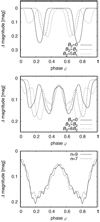 |
Fig. 6 Light curves due to the light absorption in circumstellar magnetospheres for i = β = π∕2. Upper panel: combination of dipole and quadrupole. Middle panel: combination of quadrupole and octupole. Bottom panel: light curves due to higher-order multipoles. |
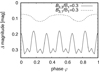 |
Fig. 7 Light curves due to the light absorption in circumstellar magnetospheres for a combination of the axisymmetric dipole and octupole with l = 3 and l = 1 for β = 0 viewed equator-on (i = π∕2). |
3.2 Continuum emission from a corotating magnetosphere
Part of the light absorbed by the corotating magnetosphere is emitted again and may reach a distant observer (Oksala et al. 2015). If the extinction appears due to light that scatters on free electrons, then the scattered light has the same spectral energy distribution as the star and there is no net absorption in the magnetosphere. However, unlike the simulation of the magnetospheric light absorption, modeling the light emission is a formidable problem. With emission, the radiative transfer equation needs to be solved in its full integro-differential form for all rays intercepting all magnetospheric points. In addition, the solution of the radiative transfer equation should be iterated for a consistent solution.
To make the problem more tractable, we did not solve the radiative transfer equation within the clouds and simply assumed that the radiation is reflected by the surface of the clouds. The amount of energy emitted by the stellar surface element d S* is F0 d S*, where F0 is the surface flux. Assuming that the stellar surface radiates according to the cosine law, the flux observed at the distance r* from the surface element is  , where θ* is the angle between the normal to the surface and the ray. A geometrically thin magnetospheric medium can be described by its cross-section with respect to the infalling radiation cosυ dS, where υ < π∕2 is an angle between the normal to the equilibrium surface element (given by ∇(f⋅b) from Eq. (1)) and the direction to the stellar surface element. The amount of radiation that is scattered by a given element is then
  . Assuming that the light is redistributed in the magnetospheric matter according to the cosine law, the flux observed at the distance d from the star is
  , where θ < π∕2 is the angle between the normal to the surface and the direction to the observer. Integrating over all stellar and equilibrium surfaces, the total observed reemitted flux relative to the flux coming from the star
  is
is
 (25)
(25)
When we numerically evaluated Eq. (25), we assumed that each surface element directly faces the star, and we accounted for occultation by the star. To simplify the calculation, the optical depth was approximated from Eq. (24) by
 (26)
(26)
The test showed that the total emitted flux calculated with this method is lower than the total absorbed flux by just a few percent. This is an acceptable difference because absorption and emission were treated differently, which is not fully compatible.
Figure 8 shows light curves due to magnetospheric emission for the case of a dipole (n = 1) with a rotational axis perpendicular to the magnetic field axis (β = 90°) and for different inclinations. The light curve due to light emission has a smooth profile and the variations appear because the line of sight changes. The minimum has a wedge-like shape with a nearly linear behavior on either side of the minima because the cos θ term appears in Eq. (25), which is roughly proportional to |cosφ |. The maxima due to each cloud are shifted with respect to the absorption minima by 0.25 in phase because the normal to the equilibrium surface is nearly perpendicular to the rotational axis and the maximum appears at the phase when the surface normal points in the direction of the observer. In contrast to the absorption, the variability appears even for a small magnetic field tilt and for a small inclination (cf. Townsend 2008).
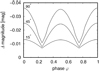 |
Fig. 8 Lightcurves due to the light emission in circumstellar magnetospheres for a dipolar magnetic field with β = 90° and different inclinations denoted in the graph. |
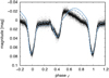 |
Fig. 9 Simulated light curve assuming a magnetic field given by the combination of a dipole and quadrupole and accounting for both absorption and emission in the magnetosphere (dashed line). The solid line corresponds to the model that also accounts for surface spots (Oksala et al. 2015). This is compared with the observed light curve of σ Ori E (Townsend et al. 2013) and phased with the ephemeris from Townsend et al. (2010). |
4 Application to stars with warped light curves
4.1 Star σ Ori E
The enigmatic light curve of σ Ori E (Hesser et al. 1976, see also Fig. 9) motivated several studies that interpreted its light variability as the result ofabsorption in the circumstellar magnetosphere (Landstreet & Borra 1978; Nakajima 1985; Preuss et al. 2004; Townsend et al. 2005). The light curve shows two deep minima that originate from the absorption in the stellar magnetosphere and from additional variability between the minima, possibly due to the light scattering (Oksala et al. 2015). With respect to the light curves of other chemically peculiar stars, it might be regarded as a warped light curve at its extrema.
We modeled the light curve assuming an inclination i = 75°, which roughly corresponds to observations (Oksala et al. 2015), and a magnetic field tilt β =90°. We selected a higher value of the tilt than derived from magnetic maps (Oksala et al. 2015) to obtain a light curve maximum height that agrees with observations. As a result of the magnetic field tilt, the circumstellar matter is not distributed axisymmetrically, but mostly appears at the intersection of the rotational and magnetic equatorial surfaces (Townsend et al. 2005). This results in two circumstellar clouds that periodically occult the stellar surface, leading to the light curves with two minima. To fit the width of the minima, we assumed the magnetospheric density parameter ρm = Aξ−3. This corresponds to the stellar wind attenuation in a dipolar field and gives a slower decrease in density than predicted by the model of a centrifugal breakout (Owocki et al. 2020) that we used in our previous calculations. This particular choice of the radial power-law index is also motivated by observational data. A higher index of the radial power law predicts a wider occultation phase than observed because most of the absorption appears closer to the star. The observed minima do not appear shifted by 0.5 in phase, which indicates that the magnetospheric matter is not distributed symmetrically (Townsend et al. 2005). Therefore, we assumed a combination of the dipolar and quadrupolar components B2 ∕B1 = 0.6 to shift the equilibrium surface (see Fig. 3) and consequently also the light minima in accordance with observations. A similar approach was used by Oksala et al. (2015). Additionally, we introduced a dependence of the density parameter A on a position to account for different depths of light minima. We assumed that the value of A in one half-space of the magnetosphere is half that in the second half-space.
The simulated light curve in Fig. 9 reproduces the main features of the observed light curve, although some details remain unexplained. The deep minima are nicely reproduced. The variations between the minima can be interpreted as due to the light scattering in the magnetosphere. As a result of the shift in the equilibrium surface introduced above, only one side of the surface is illuminated by the star, therefore the light curve due to the scattering contains only one maximum. This broad maximum appears around the phase φ = 0.7 and is the only effect in the light curve due to the light scattering. From this it follows that the quadrupolar component is needed not only to shift the light minima in phase, but also to explain the different heights of the local maxima in the light curves. Compared to the circumstellar density distribution determined by Oksala et al. (2015), the density distribution is asymmetric because of the variation in A parameter that we adopted, and it is more aligned with the rotational axis.
The shift between the predicted and observed maxima of about 0.2 in phase (Fig. 9) remains to be explained. It likely appears because the shape of the equilibrium surface is more complex than expected. We have not been able to explain this shift by variations in any magnetospheric parameters, including different orders of multipole, their mutual strength, and magnetic field inclination. The shift between primary minima and maxima due to emission is nearly 0.5 in phase, which means that it can be explained by assuming that the surface around which the magnetospheric cloud accumulates is perpendicular to the radial direction (i.e., the surface forms a small section of a sphere). A similar model was introduced to explain the continuum polarization in this star (Carciofi et al. 2013). The adopted model of geometrically thin clouds perhaps oversimplifies the situation.
The model of two clouds connected by a ring proposed by Carciofi et al. (2013) might be interpreted assuming a nonaxisymmetric field with n = l = 1. This model leads to the appearance of two flaring regions, which would explain the two deep minima. The flaring regions are extended in the direction perpendicular to the radial direction, therefore the extrema due to light emission and absorption coincide in phase.
Oksala et al. (2015) introduced another component of the light variability of σ Ori E due to abundance spots that appear on the surface of this star and that can be revealed from Doppler mapping. The abundance spots dominate the light variability in the ultraviolet domain to a great extent, and they manifest themselves as an additional shallow light maximum around phase 0.9 in the optical region. Accounting for the spots in our model has a small impact in the light curve, except for a slight shift of the light maximum toward a higher phase (Fig. 9).
We aimed to determine a magnetic field distribution that was able to reproduce not only eclipses, but also the height of the emission-like feature around phase φ = 0.6. In turn, the resulting surface magnetic field poorly agrees with the observed longitudinal magnetic field curve. This again indicates that further improvement of the magnetospheric model is required.
4.2 HD 37776 and other stars with warped light curves
The light curve of HD 37776 can mostly be explained as a result of flux redistribution in surface abundance patches of helium and silicon (Krtička et al. 2007). A detailed inspection of the HD 37776 light curve derived with the TESS satellite, however, revealed about ten localized narrow features that can be interpreted in the form of dips (warps; Mikulášek et al. 2020, Fig. 10) with additional substructures. Mikulášek et al. (2020) succeeded in providing a detailed phenomenological model of the HD 37776 TESS light curve, but the physical origin of the fine structure remained unclear. The star shows a complex magnetic field (Thompson & Landstreet 1985) with a dominating octupolar component (Kochukhov et al. 2011) and a significant nonpotential field (rot B≠0). Some of the strong warps might be attributed to the dominating l = 3 nonaxisymmetric component of the field. This component should give rise to six warps, which is slightly fewer warps than derived from observations.
This is illustrated in Fig. 10, where we plot HD 37776 light curve1 simulated by Krtička et al. (2007) from the Khokhlova et al. (2000) abundance maps, which was further modulated by circumstellar absorption due to n = 3 and l = 3 aligned multipoles (β = 0). In Sect. 2.4 we identified additional equilibrium planes cos(lϕ) = 0 that intersect the magnetic field axis. These surfaces appear in the region in which the equilibrium disk flares, therefore wedid not account for the variability induced by them. The comparison with the light curve derived using the TESS satellite (Ricker et al. 2015) shows slightly higher amplitude of the simulated data. This might be attributed to a missing iron opacity, which was not accounted for in our atmosphere modeling that we used to determine emergent fluxes, and it can compete with other opacity sources. Inclusion of circumstellar absorption better reproduces the overall shape of the light curve, although many details are missing, which indicates that shape of the magnetosphere might be more complex. This might be connected with additional components of the magnetic field. Alternatively, the light curve could be interpreted as a result of light absorption on the equilibrium surface of low-order axisymmetric multipoles (dipole or quadrupole) warped by a higher-order nonaxisymmetric multipole. We also note that the adopted magnetic field model was not selected to reproduce the surface magnetic field distribution derived from spectropolarimetry, and a more realistic magnetic field model may fit the observed light curve better.
The magnetic fields of most magnetic, chemically peculiar stars are dominated by the dipolar component already at the stellar surface (Bychkov et al. 2005; Aurière et al. 2007; Rusomarov et al. 2015; Shultz et al. 2018; Kochukhov et al. 2019), and stars in which higher-order multipoles prevail are scarce (Thompson & Landstreet 1985; Donati et al. 2006; Bailey et al. 2012; Yakunin et al. 2015). In stars with purely dipolar components, simple light curves with at most two absorption dips are predicted, such as that found in σ Ori E (Townsend et al. 2005). More complex light curves can appear in stars in which the higher-order multipoles dominate not only at the stellar surface, but at the Keplerian radius, where the clouds start to form. This is an even more strict condition than a dominance at the stellar surface caused by the radial decrease of higher-order multipoles, which is faster than for a pure dipole.
It follows from this that the multiple warps in the light curves of stars with prevailing dipolar magnetic field need to be explained by something else than the axisymmetric model of a rigidly rotating dipolar magnetosphere. For instance, the perturbation of an otherwise dominant axisymmetric field by even a weak nonaxisymmetric component leads to the appearance of warps on the equilibrium surface (Fig. 5) that may cause dips in the light curve (Fig. 7). Given the dominance of dipolar fields among magnetic, chemically peculiar stars, this appears to be the most promising model of the nature of the tiny features in the light curves of chemically peculiar stars.
On the other hand, if the magnetic field in the outer parts of the magnetosphere has a more complex topology than a simple dipole and is, for instance, governed by higher-order multipoles or has a component with a significant nonaxisymmetric term or with nonzero rotation, then this field may lead to a more complex distribution of magnetospheric matter and to the appearance of warps in the light curve. In the context of stellar interiors, Braithwaite & Nordlund (2006) showed with their numerical simulations that stable internal fields are not composed just from axisymmetric dipole, but also include a significant toroidal component. Magnetic field components with nonzero rotation may appear, for example, due to outflows or due to electric currents flowing in the magnetosphere. In this case, the explanation of warps by corotating magnetospheric clouds might be possible even for stars with simple surface fields. We additionally tested this possibility and simulated the light curve due to a magnetosphere governed by higher-order multipoles with accumulating clouds located in the outer regions of magnetosphere. The derived light curves resembled the warped light curves, giving this possibility some credit.
Magnetic Doppler imaging has unveiled a magnetic field with nonzero rotation in some hot stars (Kochukhov et al. 2004, 2011; Donati et al. 2006), which might indicate nonzero electric currents. We tested the possibility that these currents may be generated by nonzero velocity differences between oppositely charged particles in line-driven wind. We used our multicomponent wind models (Krtička & Kubát 2001) to estimate the magnitude of the electric current in B star winds. Our models showed that the magnetic fields induced by wind currents are weaker by several orders of magnitude than the field observed in magnetic, hot stars. Therefore, it is more likely that the magnetic fields with nonzero rotation are connected with atmospheric currents (Woltjer 1971; Rakosch et al. 1974) that are thought to contribute to hydrogen and helium line profile variations (Madej 1983; Valyavin et al. 2004; Vallverdú et al. 2014).
If the magnetospheric clouds appear at larger distances where the magnetic field no longer corresponds to a dipole, then the centrifugal acceleration dominates gravity in these regions. The vertical scale height at large distances is given by
 (27)
(27)
In other words, as a result of the linear increase in centrifugal acceleration with radius, the vertical scale height is inversely proportional to radius. Therefore, we expect larger clouds close to the star and smaller ones at large radii.
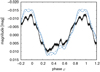 |
Fig. 10 Simulated light curve of HD 37776 derived assuming the silicon and helium surface distribution by Khokhlova et al. (2000) and modulated by n = 3 and l = 3 multipole (solid line). This is compared with the TESS light curve phased with the nonlinear ephemeris from Mikulášek et al. (2020, dots) and with the light curve calculated purely from surface spots (dashed line). All light curves were shifted to derive a zero mean magnitude. |
5 Discussion: Other possible sources of complex light variations
Matter cannot be supported by continuum radiation. This can be seen from evaluating the maximum mass that can be supported radiatively, which is given by the balance of the gravitational and radiative force  , where Σ is the column mass. The optical depth of thismaterial is given by
  . Therefore, the optical depth is given by the Eddington parameter, which is Γ <1 for normal stars. Consequently, a star cannot radiatively support material that is optically thick due to Thomson scattering.
Some stars show a complex magnetic field structure just above the stellar surface, with magnetic field lines closing significantly below the Keplerian corotation radius (e.g., Kochukhov & Wade 2016). These structures do not necessarily lead to corotating clouds supported by centrifugal force, as studied here. Instead, the field lines may be filled with wind material, which collides with streams from the opposite footpoint of the magnetic loop (Ud-Doula et al. 2008; Petit et al. 2013). This leads to the appearance of a dynamical magnetosphere with a complex upflow and downflow structure. These structures are inevitably unstable. However, because the flow along different loops is independent, the combination of absorption from a large number of loops may lead to a more or less time-independent photometric signature even for a dynamical magnetosphere. Moreover, this effect might be stronger in cooler stars with a lower wind density because the cooling time in these stars is longer and the post-shock gas is able to occult a larger fraction of the stellar surface.
The density of the post-shock in nearly isobaric matter can be estimated as (Owocki et al. 2016)
 (28)
(28)
where ρw is the wind density, Ts is the shock temperature, and Th is the temperature of the cooled post-shock gas. The Thomson scattering optical depth due to this structures is
 (29)
(29)
where Rh is the length corresponding to the post-shock gas, and vw is the wind velocity. Because Ts∕Th may be up to 103, the dynamical magnetosphere may affect the light curve only for stars with a higher mass-loss rate Ṁ ≳ 10−10 M⊙ yr−1. This overcomes the mass-loss rates of a typical chemically peculiar star by several orders of magnitude (Krtička 2014).
It is also possible consider the problem of the shock-heated magnetospheres (Babel & Montmerle 1997; ud-Doula et al. 2014)from the point of view of X-ray energetics. The density scale height at these temperatures is comparable to the stellar radius, therefore this matter is close to the hydrostatic equilibrium along the field lines (Owocki et al. 2016). The denser structures in this environment may give rise to the warped light curves. The hot magnetospheric matter needs to obscure about δ = 10−3 of stellar radiation to cause warp features with an amplitude of about 1 mmag. This gives the condition for the minimum density of this material as σTρC∕mH ≈ δ, where C denotes the length of the cloud in the direction of observation. This implies that the mass of the cloud ABmHδ∕σT must be about 10−14 M⊙ assuming the cloud dimensions A ≈ B ≈ R* and the total mass of this corona-like structure of 10−13 M⊙ with about ten such clouds. The X-ray luminosity of such a cloud would be about  , which, using the unity optical depth condition and assuming B ≈ C, gives an X-ray luminosity of
  . The X-ray cooling function Λ from Schure et al. (2009) gives LX ≈ 1031 erg s−1, which is higher by two to three orders of magnitude than the typical luminosity of magnetic B stars (Nazé et al. 2014) and cannot be sustained by the weak winds of late-B stars.
Prominence-like structures (e.g., Sudnik & Henrichs 2016) may provide an analogy for the proposed model of matter distribution leading to dips in the light curves. Classical solar prominence models (Kippenhahn & Schlüter 1957; Kuperus & Raadu 1974) nicely correspond to structures that may cause warped light curves. The potential extrapolation of surface fields in cool stars showed that equilibrium regions may exist even below the Keplerian radius (Jardine et al. 2001) if the field is sufficiently complex. However, the height of these structures would have to be comparable to the stellar radius to cause warp features, which again requires higher-order multipoles.
6 Conclusions
We simulated light curves due to light absorption and emission in the matter that is centrifugally supported in magnetospheres for a magnetic field governed by higher orders of multipolar expansion. Our aim was to understand the complex light curves of chemically peculiar stars, which show persistent phased multiple features that can be interpreted as dips (warps).
We have shown that with increasing order of the multipolar expansion of the magnetic field, the complexity of the light curve increases. Two warps at most appear per order of multipolar expansion for axisymmetric fields. However, higher-order axisymmetric multipoles have to dominate not only at the stellar radius, but also at the Keplerian radius to significantly affect the light curve. A similar condition was found by Jardine et al. (2001) for the existence of prominences in cool stars. Because most of the hot, magnetic stars do not show these intricate surface fields, complex warped light curves originating from complicated surface fields are expected to be rare. A study is under way to test this prediction (Mikulášek et al., in prep.).
We distinguished two geometrically different sources of variability. For axially symmetric magnetic fields, the resulting distribution of magnetospheric matter retains some kind of symmetry, therefore a nonzero tilt between the magnetic and rotational axes is needed to obtain some light variability. In this case, the variability occurs because the star is occulted by a geometrically thin magnetospheric disk that moves across the visible surface. This leads to strong warps in the light curve, which appear, for example, in σ Ori E.
On the other hand, for nonaxisymmetric fields, the variability appears even when the magnetic and rotational axis coincide. In this case, the disk geometrically flares and warps in the light curve are caused by the occultation of a large part of the stellar surface by the flaring disk. The occulting matter is typically optically thin, which leads to weak dips such as that observed in HD 37776.
A combination of low-order axisymmetric multipole with weak higher-order nonaxisymmetric multipoles leads to the warping of the originally symmetric equilibrium structure. This could appear even in typical magnetic, hot stars, which are dominated by a dipolar field. This combination of axisymmetric and non-axisymmetric multipoles might introduce structures that can explain the tiny features observed in the light curves of chemically peculiar stars.
Acknowledgements
The authors thank Profs. O. Kochukhov and S. P. Owocki for the discussion of the topic and an anonymous referee for valuable comments which helped us to significantly improve the paper.
References
- Abbott, D. C. 1979, IAU Symp., 83, 237 [NASA ADS] [Google Scholar]
- Adelman, S. J. 2006, PASP, 118, 77 [NASA ADS] [CrossRef] [Google Scholar]
- Alecian, G., & Stift, M. J. 2017, MNRAS, 468, 1023 [Google Scholar]
- Aurière, M., Wade, G. A., Silvester, J., et al. 2007, A&A, 475, 1053 [NASA ADS] [CrossRef] [EDP Sciences] [Google Scholar]
- Babel, J. 1995, A&A, 301, 823 [Google Scholar]
- Babel, J. 1996, A&A, 309, 867 [Google Scholar]
- Babel, J., & Montmerle, T. 1997, A&A, 323, 121 [NASA ADS] [Google Scholar]
- Bailey, J. D., Grunhut, J., Shultz, M., et al. 2012, MNRAS, 423, 328 [NASA ADS] [CrossRef] [Google Scholar]
- Braithwaite, J., & Nordlund, Å. 2006, A&A, 450, 1077 [NASA ADS] [CrossRef] [EDP Sciences] [Google Scholar]
- Bychkov, V. D., Bychkova, L. V., & Madej, J. 2005, A&A, 430, 1143 [NASA ADS] [CrossRef] [EDP Sciences] [Google Scholar]
- Carciofi, A. C., Faes, D. M., Townsend, R. H. D., & Bjorkman, J. E. 2013, ApJ, 766, L9 [NASA ADS] [CrossRef] [Google Scholar]
- Castor, J. I., Abbott, D. C., & Klein, R. I. 1975, ApJ, 195, 157 [Google Scholar]
- Donati, J. F., Howarth, I. D., Jardine, M. M., et al. 2006, MNRAS, 370, 629 [NASA ADS] [CrossRef] [Google Scholar]
- Grunhut, J. H., Rivinius, T., Wade, G. A., et al. 2012, MNRAS, 419, 1610 [CrossRef] [Google Scholar]
- Hesser, J. E., Walborn, N. R., & Ugarte, P. P. 1976, Nature, 262, 116 [NASA ADS] [CrossRef] [Google Scholar]
- Hümmerich, S., Mikulášek, Z., Paunzen, E., et al. 2018, A&A, 619, A98 [NASA ADS] [CrossRef] [EDP Sciences] [Google Scholar]
- Jagelka, M., Mikulášek, Z., Hümmerich, S., & Paunzen, E. 2019, A&A, 622, A199 [NASA ADS] [CrossRef] [EDP Sciences] [Google Scholar]
- Jardine, M., Barnes, J. R., Donati, J.-F., & Collier Cameron, A. 1999, MNRAS, 305, L35 [NASA ADS] [CrossRef] [Google Scholar]
- Jardine, M., Collier Cameron, A., Donati, J. F., & Pointer, G. R. 2001, MNRAS, 324, 201 [NASA ADS] [CrossRef] [Google Scholar]
- Khokhlova, V. L., Vasilchenko, D. V., Stepanov, V. V., & Romanyuk, I. I. 2000, Astron. Lett., 26, 177 [NASA ADS] [CrossRef] [Google Scholar]
- Kippenhahn, R., & Schlüter, A. 1957, ZAp, 43, 36 [NASA ADS] [Google Scholar]
- Kochukhov, O., & Ryabchikova, T. A. 2018, MNRAS, 474, 2787 [NASA ADS] [CrossRef] [Google Scholar]
- Kochukhov, O., & Wade, G. A. 2016, A&A, 586, A30 [NASA ADS] [CrossRef] [EDP Sciences] [Google Scholar]
- Kochukhov, O., Bagnulo, S., Wade, G. A., et al. 2004, A&A, 414, 613 [NASA ADS] [CrossRef] [EDP Sciences] [Google Scholar]
- Kochukhov, O., Lundin, A., Romanyuk, I., & Kudryavtsev, D. 2011, ApJ, 726, 24 [NASA ADS] [CrossRef] [Google Scholar]
- Kochukhov, O., Shultz, M., & Neiner, C. 2019, A&A, 621, A47 [NASA ADS] [CrossRef] [EDP Sciences] [Google Scholar]
- Krtička J. 2014, A&A, 564, A70 [NASA ADS] [CrossRef] [EDP Sciences] [Google Scholar]
- Krtička, J., & Kubát, J. 2001, A&A, 377, 175 [NASA ADS] [CrossRef] [EDP Sciences] [Google Scholar]
- Krtička, J., Mikulášek, Z., Zverko, J., & Žižňovský, J. 2007, A&A, 470, 1089 [NASA ADS] [CrossRef] [EDP Sciences] [Google Scholar]
- Krtička, J., Mikulášek, Z., Henry, G. W., et al. 2009, A&A, 499, 567 [NASA ADS] [CrossRef] [EDP Sciences] [Google Scholar]
- Kuperus, M., & Raadu, M. A. 1974, A&A, 31, 189 [NASA ADS] [Google Scholar]
- Landstreet, J. D., & Borra, E. F. 1978, ApJ, 224, L5 [NASA ADS] [CrossRef] [Google Scholar]
- Leto, P., Trigilio, C., Buemi, C. S., Umana, G., & Leone, F. 2006, A&A, 458, 831 [NASA ADS] [CrossRef] [EDP Sciences] [Google Scholar]
- Madej, J. 1983, Acta Astron., 33, 1 [NASA ADS] [Google Scholar]
- Michaud, G. 1970, ApJ, 160, 641 [Google Scholar]
- Mikulášek, M., Zverko, J., Krtička, J., et al. 2007, in Physics of Magnetic Stars, eds. I. I. Romanyuk, D. O. Kudryavtsev, O. M. Neizvestnaya, & V. M. Shapoval (USA: ASP Books), 300 [Google Scholar]
- Mikulášek, Z., Krtička, J., Henry, G. W., et al. 2008, A&A, 485, 585 [NASA ADS] [CrossRef] [EDP Sciences] [Google Scholar]
- Mikulášek, Z., Krtička, J., Shultz, M. E., et al. 2020, in Stellar Magnetism: A Workshop in Honour of the Career and Contributions of John D. Landstreet, ed. G. Wade, E. Alecian, D. Bohlender, & A. Sigut, 11, 46 [Google Scholar]
- Molnar, M. R. 1973, ApJ, 179, 527 [NASA ADS] [CrossRef] [Google Scholar]
- Nakajima, R. 1985, Ap&SS, 116, 285 [NASA ADS] [Google Scholar]
- Nazé, Y., Petit, V., Rinbrand, M., et al. 2014, ApJS, 215, 10 [CrossRef] [Google Scholar]
- Oksala, M. E., Wade, G. A., Marcolino, W. L. F., et al. 2010, MNRAS, 405, L51 [NASA ADS] [CrossRef] [Google Scholar]
- Oksala, M. E., Kochukhov, O., Krtička, J., et al. 2015, MNRAS, 451, 2015 [Google Scholar]
- Owocki, S. P., & Cranmer, S. R. 2018, MNRAS, 474, 3090 [NASA ADS] [CrossRef] [Google Scholar]
- Owocki, S. P., ud-Doula, A., Sundqvist, J. O., et al. 2016, MNRAS, 462, 3830 [NASA ADS] [CrossRef] [Google Scholar]
- Owocki, S. P., Shultz, M. E., ud-Doula, A., et al. 2020, MNRAS, 499, 5366 [NASA ADS] [CrossRef] [Google Scholar]
- Peterson, D. M. 1970, ApJ, 161, 685 [NASA ADS] [CrossRef] [Google Scholar]
- Petit, V., Owocki, S. P., Wade, G. A., et al. 2013, MNRAS, 429, 398 [NASA ADS] [CrossRef] [Google Scholar]
- Preuss, O., Schüssler, M., Holzwarth, V., & Solanki, S. K. 2004, A&A, 417, 987 [NASA ADS] [CrossRef] [EDP Sciences] [Google Scholar]
- Prvák, M. 2019, PhD thesis, Masaryk University, Czechia, https://is.muni.cz/th/onlb4/phd.pdf [Google Scholar]
- Prvák, M., Liška, J. Krtička, J., Mikulášek, Z., & Lüftinger, T. 2015, A&A, 584, A17 [NASA ADS] [CrossRef] [EDP Sciences] [Google Scholar]
- Rakosch, K. D., Sexl, R., & Weiss, W. W. 1974, A&A, 31, 441 [NASA ADS] [Google Scholar]
- Ricker, G. R., Winn, J. N., Vanderspek, R., et al. 2015, J. Astron. Telesc. Instrum., Syst., 1, 014003 [Google Scholar]
- Rusomarov, N., Kochukhov, O., Ryabchikova, T., & Piskunov, N. 2015, A&A, 573, A123 [NASA ADS] [CrossRef] [EDP Sciences] [Google Scholar]
- Schure, K. M., Kosenko, D., Kaastra, J. S., Keppens, R., & Vink, J. 2009, A&A, 508, 751 [NASA ADS] [CrossRef] [EDP Sciences] [Google Scholar]
- Shultz, M. E., Wade, G. A., Rivinius, T., et al. 2018, MNRAS, 475, 5144 [NASA ADS] [Google Scholar]
- Shultz, M., Rivinius, T., Das, B., Wade, G. A., & Chandra, P. 2019a, MNRAS, 486, 5558 [CrossRef] [Google Scholar]
- Shultz, M. E., Wade, G. A., Rivinius, T., et al. 2019b, MNRAS, 490, 274 [NASA ADS] [CrossRef] [Google Scholar]
- Shultz, M. E., Owocki, S., Rivinius, T., et al. 2020, MNRAS, 499, 5379 [NASA ADS] [CrossRef] [Google Scholar]
- Shulyak, D., Krtička, J., Mikulášek, Z., Kochukhov, O., & Lüftinger, T. 2010, A&A, 524, A66 [CrossRef] [EDP Sciences] [Google Scholar]
- Silvester, J., Kochukhov, O., Rusomarov, N., & Wade, G. A. 2017, MNRAS, 471, 962 [NASA ADS] [CrossRef] [Google Scholar]
- Smith, M. A.,& Groote, D. 2001, A&A, 372, 208 [NASA ADS] [CrossRef] [EDP Sciences] [Google Scholar]
- Sudnik, N. P.,& Henrichs, H. F. 2016, A&A, 594, A56 [NASA ADS] [CrossRef] [EDP Sciences] [Google Scholar]
- Thompson, I. B., & Landstreet, J. D. 1985, ApJ, 289, L9 [NASA ADS] [CrossRef] [Google Scholar]
- Townsend, R. H. D. 2008, MNRAS, 389, 559 [NASA ADS] [CrossRef] [Google Scholar]
- Townsend, R. H. D., & Owocki, S. P. 2005, MNRAS, 357, 251 [NASA ADS] [CrossRef] [Google Scholar]
- Townsend, R. H. D., Owocki, S. P., & Groote, D. 2005, ApJ, 630, L81 [NASA ADS] [CrossRef] [Google Scholar]
- Townsend, R. H. D., Oksala, M. E., Cohen, D. H., Owocki, S. P., & ud-Doula, A. 2010, ApJ, 714, L318 [NASA ADS] [CrossRef] [Google Scholar]
- Townsend, R. H. D., Rivinius, T., Rowe, J. F., et al. 2013, ApJ, 769, 33 [NASA ADS] [CrossRef] [Google Scholar]
- Trigilio, C., Leto, P., Umana, G., Leone, F., & Buemi, C. S. 2004, A&A, 418, 593 [NASA ADS] [CrossRef] [EDP Sciences] [Google Scholar]
- ud-Doula, A., & Owocki, S. P. 2002, ApJ, 576, 413 [NASA ADS] [CrossRef] [Google Scholar]
- Ud-Doula, A., Owocki, S. P., & Townsend, R. H. D. 2008, MNRAS, 385, 97 [NASA ADS] [CrossRef] [Google Scholar]
- ud-Doula, A., Owocki, S., Townsend, R., Petit, V., & Cohen, D. 2014, MNRAS, 441, 3600 [NASA ADS] [CrossRef] [Google Scholar]
- Vallverdú, R., Cidale, L., Rohrmann, R., & Ringuelet, A. 2014, Ap&SS, 352, 95 [Google Scholar]
- Valyavin, G., Kochukhov, O., & Piskunov, N. 2004, A&A, 420, 993 [NASA ADS] [CrossRef] [EDP Sciences] [Google Scholar]
- Vauclair, S., Dolez, N., & Gough, D. O. 1991, A&A, 252, 618 [NASA ADS] [Google Scholar]
- Vick, M., Michaud, G., Richer, J., & Richard, O. 2011, A&A, 526, A37 [NASA ADS] [CrossRef] [EDP Sciences] [Google Scholar]
- Wolff, S. C., & Wolff, R. J. 1971, AJ, 76, 422 [NASA ADS] [CrossRef] [Google Scholar]
- Woltjer, L. 1971, PASP, 83, 592 [NASA ADS] [CrossRef] [Google Scholar]
- Yakunin, I., Wade, G., Bohlender, D., et al. 2015, MNRAS, 447, 1418 [NASA ADS] [CrossRef] [Google Scholar]
The detailed ephemeris will be published elsewhere (Mikulášek et al., in prep.). The phase of the adopted nonlinear ephemeris can be approximated as  , where ϑ0 = (t − M0)∕P0.
P0 = 1.538 736(2) days,
Ṗ0 = −1.51(4) × 10−8,
, where ϑ0 = (t − M0)∕P0.
P0 = 1.538 736(2) days,
Ṗ0 = −1.51(4) × 10−8,
 d−1, and M0 = 2 459 580.715(5).
All Figures
|
Fig. 1 Equilibrium surfaces Eq. (1) fulfilling the stability condition Eq. (4) for a field aligned with the stellar rotational axis and multipoles with different orders. |
| In the text | |
|
Fig. 2 Equilibrium surfaces Eq. (1) fulfilling the stability condition Eq. (4) for a rotational axis ω tilted by 5∕12 π with respect to the axis of the magnetic field b for multipoles with different orders. Both axes are denoted in the graph. |
| In the text | |
|
Fig. 3 Equilibrium surfaces fulfilling the stability condition for a field aligned with the rotational axis and a combination of multipoles with different orders. |
| In the text | |
|
Fig. 4 Magnetic field vector for the dipolar (blue) and quadrupolar (red) field plotted in the y = 0 plane. The dipolar component is plotted with the unit length vector, and the length of the quadrupolar field vector is reduced by afactor of 1∕ξ. |
| In the text | |
|
Fig. 5 Equilibrium surface fulfilling the stability condition for a field aligned with the rotational axis and combination of the axisymmetric dipole and octupole with l = 2 (upper panel) and l = 3 (lower panel). Plotted for B3,2∕B1 = 0.3 or B3,3 ∕B1 = 0.3. |
| In the text | |
|
Fig. 6 Light curves due to the light absorption in circumstellar magnetospheres for i = β = π∕2. Upper panel: combination of dipole and quadrupole. Middle panel: combination of quadrupole and octupole. Bottom panel: light curves due to higher-order multipoles. |
| In the text | |
|
Fig. 7 Light curves due to the light absorption in circumstellar magnetospheres for a combination of the axisymmetric dipole and octupole with l = 3 and l = 1 for β = 0 viewed equator-on (i = π∕2). |
| In the text | |
|
Fig. 8 Lightcurves due to the light emission in circumstellar magnetospheres for a dipolar magnetic field with β = 90° and different inclinations denoted in the graph. |
| In the text | |
|
Fig. 9 Simulated light curve assuming a magnetic field given by the combination of a dipole and quadrupole and accounting for both absorption and emission in the magnetosphere (dashed line). The solid line corresponds to the model that also accounts for surface spots (Oksala et al. 2015). This is compared with the observed light curve of σ Ori E (Townsend et al. 2013) and phased with the ephemeris from Townsend et al. (2010). |
| In the text | |
|
Fig. 10 Simulated light curve of HD 37776 derived assuming the silicon and helium surface distribution by Khokhlova et al. (2000) and modulated by n = 3 and l = 3 multipole (solid line). This is compared with the TESS light curve phased with the nonlinear ephemeris from Mikulášek et al. (2020, dots) and with the light curve calculated purely from surface spots (dashed line). All light curves were shifted to derive a zero mean magnitude. |
| In the text | |
Current usage metrics show cumulative count of Article Views (full-text article views including HTML views, PDF and ePub downloads, according to the available data) and Abstracts Views on Vision4Press platform.
Data correspond to usage on the plateform after 2015. The current usage metrics is available 48-96 hours after online publication and is updated daily on week days.
Initial download of the metrics may take a while.