| Issue |
A&A
Volume 674, June 2023
|
|
|---|---|---|
| Article Number | A94 | |
| Number of page(s) | 8 | |
| Section | Stellar structure and evolution | |
| DOI | https://doi.org/10.1051/0004-6361/202245551 | |
| Published online | 07 June 2023 | |
EPIC 206197016: A very hot white dwarf orbited by a strongly irradiated red dwarf⋆
1
Department of Theoretical Physics and Astrophysics, Faculty of Science, Masaryk University, Kotlářská 2, Brno, Czech Republic
e-mail: This email address is being protected from spambots. You need JavaScript enabled to view it.
2
International Centre for Radio Astronomy Research, Curtin University, Perth, Australia
3
Space Research Institute, Austrian Academy of Sciences, Schmiedlstrasse 6, Graz, Austria
Received:
25
November
2022
Accepted:
23
April
2023
Abstract
Context. Very precise satellite photometry has revealed a large number of variable stars whose variability is caused either by surface spots or by binarity. Detailed studies of such variables provide insights into the physics of these objects.
Aims. We study the nature of the periodic light variability of the white dwarf EPIC 206197016 that was observed by the K2 mission.
Methods. We obtain phase-resolved medium-resolution spectroscopy of EPIC 206197016 using X-shooter spectrograph at VLT to understand the nature of the white dwarf variability. We use non-local thermodynamical equilibrium model atmospheres to determine stellar parameters at individual phases.
Results. EPIC 206197016 is a hot DA white dwarf with Teff = 78 kK. The analysis of the spectra reveals periodic radial velocity variations that can result from gravitational interaction with an invisible secondary whose mass corresponds to a red dwarf. The close proximity of the two stars where the semimajor axis is about 3 R⊙ results in the irradiation of the companion with temperatures more than twice as high on the illuminated side compared to the nonilluminated hemisphere. This effect can explain the observed light variations. The spectra of the white dwarf show a particular feature of the Balmer lines called the Balmer line problem, where the observed cores of the lower Balmer lines are deeper than predicted. This can be attributed to either weak pollution of hydrogen in the white dwarf atmosphere by heavy elements or to the presence of a circumstellar cloud or disk.
Key words: white dwarfs / stars: variables: general / binaries: spectroscopic / stars: atmospheres
Based on observations collected at the European Southern Observatory, Paranal, Chile (ESO programme 0103.D-0194(A)).
© The Authors 2023
 Open Access article, published by EDP Sciences, under the terms of the Creative Commons Attribution License (https://creativecommons.org/licenses/by/4.0), which permits unrestricted use, distribution, and reproduction in any medium, provided the original work is properly cited.
This article is published in open access under the Subscribe to Open model. This email address is being protected from spambots. You need JavaScript enabled to view it. to support open access publication.
1. Introduction
In a multiple stellar system, extrinsic light variability typically appears due to geometrical reasons, either as a result of stellar rotation or orbital motion. The periodic nature of this variability enables us to learn about the geometry of a studied object that would otherwise probably remain unresolved.
Rotational light variability is very common among stars of different spectral types. From cool to hot, many stars show photometric spots or patches, which cause light variability as a result of stellar rotation (e.g., Walkowicz & Basri 2013; Hümmerich et al. 2016; Cunha et al. 2019; Sikora et al. 2019; Momany et al. 2020). However, the physical nature of photometric spots may differ for stars with different spectral types. While the presence of spots in cool stars is connected with the convective flux being suppressed in regions with strong magnetic fields (Isik et al. 2007; Yadav et al. 2015), patches on hot stars appear most frequently as a result of flux redistribution in abundance spots (Peterson 1970; Wolff & Wolff 1971; Trasco 1972).
Light variations due to rotation have also been detected in white dwarfs. Dupuis et al. (2000) found periodic extreme ultraviolet variability in the DA white dwarf GD 394, which was attributed to a silicon surface spot. More recently, Wilson et al. (2020) detected optical variations of this star from Transiting Exoplanet Survey Satellite (TESS) observations. In many cases, the nature of light variability of white dwarfs is not reliably known (Williams et al. 2013; Maoz et al. 2015; Pshirkov et al. 2020). Nevertheless, apart from chemical spots (Kilic et al. 2015), magnetic fields are often considered a main cause (Reding et al. 2020).
Hot white dwarfs may have surface spots as a result of radiative diffusion, which affects their outer layers (Unglaub & Bues 2000). White dwarfs accrete debris coming from their planetary systems (e.g., Brown et al. 2017), which may also lead to uneven distribution of metals across their surfaces. In strongly magnetized white dwarfs, even continuum absorption coefficients may be affected by the magnetic field (Kemp 1970; Canuto et al. 1971; Čadež & Javornik 1981), providing another possible source of light variability.
However, there are other mechanisms that may mimic the variability due to the surface spots and hamper the search for surface inhomogeneities. In many cases, variations due to binary effects, that is, ellipsoidal variations and reflection effects, may resemble spot variability (e.g., Green et al. 2023). The ellipsoidal variability appears due to tidal deformation of surfaces of binary components (Kopal 1959). This is therefore particularly important to consider when the binary separation is comparable to the radii of the individual components, for instance, in main-sequence binaries with periods of few days (e.g., Koubský et al. 2019; Kochukhov et al. 2021) or in subdwarf binaries with periods on the order of tens of minutes (e.g., Kawka et al. 2015; Kupfer et al. 2020). The so-called reflection effect appears to be due to mutual irradiation of components (Kopal 1959), and it becomes especially important in binaries with large effective temperature differences, such as in systems containing white dwarfs. For instance, reflection or reprocessing effects are seen in many close binaries where the companion of a white dwarf is either a low-mass main-sequence star (Kawka et al. 2002) or a brown dwarf (Casewell et al. 2018). For short-period systems, the light curves are modified by relativistic effects (so-called Doppler beaming, Loeb & Gaudi 2003).
To resolve these issues and to understand the nature of light variability of white dwarfs, we inspected the list of white dwarfs observed by the Kepler satellite (Hermes et al. 2017b), looking for those that may show periodic variability. We selected the most promising ones for a detailed spectroscopic study to identify their nature (Krtička et al. 2020a). In this paper, we report the detailed analysis of EPIC 206197016 (WD 2244−100, PB 7199, SDSSJ224653.72−094834.4).
2. Observations
The available astrometric and photometric data for EPIC 206197016 are summarized in Table 1. The coordinates and R magnitude were obtained from the Mikulski Archive for Space Telescopes (MAST) K2 catalog (Howell et al. 2014). The distance d was determined using the parallax from the Gaia Data Release 3 (DR3) data (Gaia Collaboration 2016, 2018; Lindegren et al. 2021).
Astrometric and photometric properties of EPIC 206197016 (top) and derived mean parameters (bottom).
We performed phase-resolved spectroscopy of EPIC 206197016 as part of the ESO proposal 0103.D-0194(A). The spectra were acquired with the X-shooter spectrograph (Vernet et al. 2011) mounted on the 8.2 m UT2 Kueyen Telescope. The spectroscopic observations are summarized in Table 2. We utilized the UVB and VIS arms, which provide an average spectral resolution (R = λ/Δλ) of 9700 and 18 400, respectively.
List of EPIC 206197016 spectra used for the analysis.
The spectra were manually calibrated and shifted to the rest frame using the radial velocities vrad (given in Table 2) determined from each spectrum by means of the cross correlation technique. We used a theoretical spectrum as a template (Zverko et al. 2007). In addition, we tested the effect of the emission peak inside the Hα profile on the determined radial velocities, but we found it to be negligible.
The K2 photometry of EPIC 206197016 was obtained from the MAST archive1 (Howell et al. 2014). The photometry shows periodic light variations, from which we determined the ephemeris (in barycenter corrected Julian date)
 (1)
(1)
using the method described by Mikulášek (2016). Here, the zero phase corresponds to the maximum of the light curve.
The observational data were supplemented with photometry derived using the Virtual Observatory SED Analyzer2 web tool (VOSA; Bayo et al. 2008), which was used to build the spectral energy distribution. We used photometry from Galaxy Evolution Explorer (GALEX; Bianchi et al. 2011), Sloan Digital Sky Survey (SDSS; Alam et al. 2015), the Carlsberg Meridian Telescope CCD drift scan survey (Evans et al. 2002), the Panoramic Survey Telescope and Rapid Response System 1 survey (Pan-STARRS1; Chambers et al. 2016), Gaia (Gaia Collaboration 2018), Visible and Infrared Survey Telescope for Astronomy survey (VISTA; Cross et al. 2012), and Wide-field Infrared Survey Explorer (WISE; Wright et al. 2010).
3. Spectroscopic analysis
3.1. Stellar parameters
We fitted the stellar spectra to derive the stellar parameters. We used the TLUSTY non-local thermodynamical equilibrium (NLTE) model atmospheres and the SYNSPEC code (Lanz & Hubeny 2003, 2007) to calculate a grid of synthetic spectra. We interpolated within calculated synthetic spectra to get the best match between theoretical and observed spectra. Visual inspection did not reveal the presence of any helium lines and pointed to a very high temperature of the star. Therefore, we selected a grid parameterized by the effective temperature Teff ∈ [70, 80, 90] kK, surface gravity logg ∈ [7.00, 7.25, 7.50, 7.75], and helium abundance εHe = log(NHe/NH)∈[10−3, 10−2] to obtain a grid of 24 NLTE models of stellar atmospheres and synthetic spectra. We did not include any elements heavier than helium into our calculations. We used both normalized and flux calibrated spectra, which gave nearly the same results.
An example of the fitted spectra is given in Fig. 1, which shows that the models are able to nicely reproduce the higher order Balmer lines and the wings of the lower order Balmer lines, while the observed cores of Hα, Hβ, and Hγ are deeper than predicted. This is a manifestation of the so-called “Balmer line problem” (Napiwotzki 1992; Werner 1996; Werner et al. 2018) wherein the observed lower Balmer lines appear stronger than the higher Balmer lines. Therefore, the lower Balmer lines can be fitted with a lower effective temperature than the higher ones. The origin of this problem is not fully clear, but it can possibly be attributed to metal line blanketing or to the presence of a circumstellar magnetosphere (Werner 1996; Vennes 1999; Werner et al. 2019). To mitigate the problem, we fit only the spectra from the UVB arm.
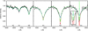 |
Fig. 1. Comparison of observed and fitted spectra. The black curve denotes observed spectrum (φ = 0.332), the blue curve corresponds to the fitted spectrum, the red curve denotes the spectrum with additional magnetospheric absorption, and the green curve denotes the spectrum from the model that includes heavy elements. The inlet shows the central part of the Hα profile. |
The final determined parameters are given in Table 1. They were determined as the average of the parameters derived from the individual UVB spectra. The derived parameters support our initial estimate that the object is a very hot DA white dwarf with no traces of helium in the atmosphere. The estimated temperature is somewhat lower than the value of 100 000 ± 4000 K determined by Tremblay et al. (2011) using similar methodology as we used here. The difference in temperature is perhaps connected with the fact that their analysis is based on spectra of lower quality.
Since the line cores are most significantly affected by the Balmer line problem, we separately fit all observed Balmer lines (including Hα) while only considering the line wings. This gives slightly more consistent parameters of Teff = 83 ± 3 kK and logg = 7.64 ± 0.07. However, these values are (within the errors) the same as those derived from the fitting of whole line profiles. This likely implies that the Balmer line problem does not significantly affect the derived stellar parameters. Furthermore, the good agreement between predicted (neglecting interstellar reddening) and observed spectral energy distribution shown in Fig. 2 also supports the reliability of the derived parameters. However, the spectral energy distribution provides just a loose constraint on the effective temperature because the fit performed using a larger grid of model atmosphere fluxes from Levenhagen et al. (2017) yields only Teff > 40 kK. The fit of the spectral energy distribution with temperature from spectroscopy gives a radius estimate of 0.021 ± 0.001 R⊙. With logg derived from spectroscopy (Table 1), this gives a stellar mass of 0.52 ± 0.12 M⊙, which is consistent with the value derived in the following analysis from evolutionary tracks within the errors. The lack of any infrared excess implies that any potential companion should be of a spectral type later than M8, as derived using the stellar parameters from Harmanec (1988, or extrapolating data from Eker et al. 2018). Because the spectral energy distribution is rather insensitive to the effective temperature of the white dwarf at observed wavelengths, this conclusion is not affected by observational uncertainties of derived parameters.
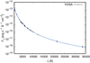 |
Fig. 2. Comparison of the predicted spectral energy distribution calculated for the determined parameters (Table 1, solid blue line) with observational data derived using the VOSA web tool (Bayo et al. 2008). |
Besides the Balmer lines, we have not found any clear evidence for the presence of other stellar lines in the spectra. We found absorption lines at 3384 Å (identified as Ti II), 3934 Å, and 3968 Å (Ca II), which are narrow and therefore likely have interstellar (or circumbinary) origin. Their origin is further supported by our analysis showing that these lines are stationary and do not change their wavelength. Furthermore, the spectra display a broad absorption feature at about 4606 Å, which we were unable to clearly identify.
From the derived effective temperature and surface gravity, we determined a mass of 0.57 M⊙ and a cooling age of 2.37 × 10⁵ yr using DA cooling tracks from the Montreal group3 (Holberg & Bergeron 2006; Bédard et al. 2020). The derived mass nicely agrees with M1 = 0.59 ± 0.02 M⊙, determined by Tremblay et al. (2011). We also checked the distance using the obtained values and the SDSS g band photometry and found it to be 560 ± 65 pc, which is consistent with the Gaia distance (Table 1), within the uncertainties.
3.2. Radial velocity curve and evolutionary status
Hermes et al. (2017a) detected radial velocity variations and suspected that EPIC 206197016 is a binary. We combined their radial velocity measurements with our determinations (Table 2) in Fig. 3. The best phasing of all radial velocities can be achieved with a period of P = 0.829168(54) d, which is slightly higher than that derived from photometry. The assumption of circular orbits provides a good fit to the radial velocity curve with semiamplitude v1 = 23 ± 4 km s−1. The mass ratio is given by
 (2)
(2)
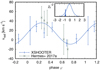 |
Fig. 3. Phase-folded X-shooter (blue) and Hermes et al. (2017a, green) radial velocity values. The data were phased with period from radial velocity variations. The inlet shows the periodogram of the radial velocity values as a function of the relative period difference ΔP/P × 104, where P is the orbital period derived from the radial velocity variations. The arrow indicates the period derived from the photometry. |
where i is the orbital inclination. With a white dwarf mass of M1 = 0.57 M⊙ and the derived semiamplitude of the radial velocities, the solution of Eq. (2) gives a secondary mass of M2 ≥ 0.06 M⊙. This corresponds to either a low-mass red dwarf or a high-mass brown dwarf. The orbital separation estimated from the third Kepler law is a > 3.1 R⊙, which is large enough to accommodate any cool main-sequence star into the system.
Comparable white dwarf binaries with a brown dwarf or a low-mass red dwarf companion have already been found (Becklin & Zuckerman 1988; Kawka & Vennes 2003; Farihi et al. 2010; Burleigh et al. 2011; Kosakowski et al. 2022). The initial-final mass relation of Cummings et al. (2018) estimates an initial mass of about 1.0 M⊙ for a white dwarf mass of M1 = 0.57 M⊙. However, the real initial mass may be significantly higher because this estimate does not take into account previous binary interaction. The stellar radius during late evolutionary phases of solar-mass stars exceeds the current separation of binary components by orders of magnitude, therefore indicating that the system has undergone a common envelope phase (Paczynski 1976; Zorotovic & Schreiber 2022).
We explored the possible evolutionary history of the system using the output from the Binary Population and Spectral Synthesis code (BPASS; Stanway & Eldridge 2018 version 2.2.1). We searched the available tracks for the system with parameters that are close to the observed values. We selected a model with the initial parameters M1 = 3 M⊙, M2 = 0.3 M⊙, and P = 6.3 d. This system passes through a contact binary phase, during which the primary loses a significant fraction of its mass (e.g., Kramer et al. 2020) and becomes a helium dominated subdwarf with a mass of 0.42 M⊙ that likely evolves into the realm of white dwarfs (this is not covered by the available track). There is still some hydrogen left on the stellar surface, and consequently, one can assume that helium later sinks down and the object appears as a hydrogen dominated DA white dwarf (Bédard et al. 2023). The orbital period of the system shrinks to about 0.6 d. The grid of evolutionary tracks does not contain systems with mass ratios lower than 0.1. Consequently, we were unable to find a model with a secondary mass close to the value estimated from the observations. However, a comparison with a track that has a higher mass of the secondary star showed that the final parameters of the primary are rather insensitive to the initial mass of the secondary. Therefore, although the final parameters do not perfectly match those of EPIC 206197016, it is reasonable to assume that a system with a lower initial mass of the secondary would evolve in a similar way and explain the final parameters better.
The binary might have experienced even more complex evolution featuring a second common envelope stage after the secondary left the main sequence (Li et al. 2023). However, this seems to be less likely, as the light variations studied in the next section do not indicate that the secondary left the main sequence.
4. Nature of the light variations
Although our test using the spot model of Prvák (2019) revealed that the observed light variations can be caused by spots, given the alleged binary nature of the object, it is more reasonable to assume a binary origin of the light variations for EPIC 206197016. In this case, the light variations could either be due to the distortion of the white dwarf surface or to reflection.
If the light variations are due to distortion of the white dwarf surface (ellipsoidal variability), then the orbital period would be twice that determined in Eq. (1). By using Kepler’s third law, the semimajor axis would be at least 4.9 R⊙. To estimate the amplitude of the ellipsoidal variability, we used our code (Krtička et al. 2020a), which within the Roche model predicts the light curve of the primary due to distortion of its surface by an accompanying secondary. Assuming a companion mass of 0.2 M⊙, the derived amplitude is three orders of magnitude lower than the observed amplitude of the light variability. Consequently, we conclude that the ellipsoidal variations due to distortion of the white dwarf are unlikely to cause light variability in EPIC 206197016.
Another possibility is that the light variations are due to a reflection effect on a white dwarf companion (e.g., Budaj 2011; Schaffenroth et al. 2019). In such a case, the orbital period would be equal to that determined in Eq. (1). For the modeling of the EPIC 206197016 light curve, we used our own code that calculates the light curve of the binary with irradiation. The code assumes spherical shape of both stars, which is reasonable due to the small radii of both components in comparison to the binary separation. We assumed that both components radiate as black bodies and that the limb darkening can be described by Lambert’s cosine law (Balian et al. 2006). The code integrates the flux over the whole secondary surface to get the magnitude of binary in a given phase. We adopted an albedo of  , which is reasonable for cool stars with deep convective envelopes (Ruciński 1969). We assumed a general elliptical orbit. The resulting light curve typically resembles a sinusoidal with sharper maxima and shallower minima (Barlow et al. 2022). Computed light curves favorably compare with data derived in the literature for other systems (Derekas et al. 2015; Devarapalli et al. 2022).
We fit the observed light curve as a function of binary and secondary parameters, that is, the orbital inclination, eccentricity e, effective temperature T2, radius R2, and mass M2 of the secondary. We fixed both the white dwarf parameters (given in Table 1) and orbital period. However, the solution was not well constrained given the large number of free parameters. Therefore, we additionally fixed the secondary effective temperature to a value roughly corresponding to the maximum one allowed by the spectral energy distribution. Using the evolutionary models of low-mass stars by Baraffe et al. (2015), this yielded an estimate of the mass of the secondary. Along with Eq. (2), this constraint allowed us to fix the orbital inclination. The resulting fit of the light curve (Fig. 4) gave secondary and orbital parameters T2 = 3000 K, M2 = 0.12 M⊙, R2 = 0.08 R⊙, i = 40°, and e = 0. The derived parameters of the secondary are reasonably close to the values derived from the evolutionary tracks of Baraffe et al. (2015), which predict an evolved 0.11 M⊙ mass star with a radius of 0.135 R⊙ and effective temperature of 2900 K. Based on these results, it follows that the secondary is most likely a red dwarf.
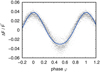 |
Fig. 4. Phase-folded light curve derived from K2 photometry. We plotted the relative difference of the observed flux from the mean value. The solid blue line is the modeled variability computed accounting for irradiation. |
As a result of irradiation, the effective temperature of the cool companion increases from about 3 kK to nearly 6 kK on its illuminated side. This significantly changes the atmospheric structure (Brett & Smith 1993; Lothringer & Casewell 2020; Lee et al. 2022), likely dissociating molecules and enhancing the atmospheric scale height (Hubeny et al. 2003). A large temperature difference between both hemispheres causes departures from hydrostatic equilibrium, resulting in a flow similar to the geostrophic flow on Earth. These effects are further modified by the energy stored in hydrogen dissociation and recombination (Tan & Komacek 2019). This might explain the slight shift between predicted and observed light minima (Fig. 4).
We did not find any signatures of the secondary in the observed spectral energy distribution (Fig. 2) nor in the spectra. The secondary can be expected to mainly dominate in the VIS part of the spectrum, which has a low signal-to-noise ratio (Table 2). This perhaps explains the missing spectral signatures of the secondary. The emission lines of the secondary could appear in the Hα line (e.g., Kawka et al. 2000, 2002), which is indeed variable. However, the emission also has contribution from the white dwarf itself (Fig. 1), which makes the analysis of this line problematic.
5. The origin of the Balmer line problem
The cores of the observed profiles of the Hα and Hβ lines of EPIC 206197016 are stronger than theory predicts. This outcome is called the Balmer line problem (Napiwotzki 1992; Werner 1996; Werner et al. 2018). To test possible periodic modulation of the Balmer line problem, we calculated the difference between the equivalent widths of predicted and observed spectra. The Balmer line core may indeed show some variability, but we consider this to be inconclusive due to a lack of correlation between variations in individual lines.
5.1. Second component
We tested if the Balmer line problem could not be explained by a combination of hot white dwarf spectrum with spectrum of another star. We tested for the presence of an additional white dwarf with stellar parameters similar to those derived for the primary star; a hot OB star, using spectra from OSTAR2002 and BSTAR2006 grids (Lanz & Hubeny 2003, 2007); and a cooler star with an effective temperature in the range of 3500 − 15 000 K, using the ATLAS9 grid (Castelli et al. 2003). The inclusion of an additional component did not lead to a significant improvement of the fit. The reason for this is that the optical region corresponds to the Rayleigh-Jeans tail of the spectra, and the combination of two spectra with similar shapes does not provide better agreement with observations. The further inclusion of a second light led to the appearance of numerous lines of the secondary (Vennes et al. 1998; Parsons et al. 2016), which do not appear in the observed spectra.
5.2. Heavy elements
Line-driven winds fade out during evolution along the white dwarf cooling track (Krtička et al. 2020b). Their disappearance opens a door for gravitational settling, which removes heavy elements from white dwarf photospheres (Unglaub & Bues 2000; Unglaub 2008) in cases where radiative levitation (Chayer et al. 1995) is inefficient. However, traces of heavy elements may still remain in the atmospheres of hot white dwarfs, possibly influencing the temperature distribution and emergent spectra. This could explain the difference between predicted and observed Balmer lines (Werner 1996; Vennes 1999; Werner et al. 2019).
To test this possibility, we prepared an additional grid of helium-free model atmospheres and synthetic spectra with Teff ∈ [80, 90] kK and logg ∈ [7.50, 7.75]. We adopted a reduced mass-fraction of heavy elements Z = 0.1 Z⊙ and fitted individual spectra with these new models. Because the presence of metals affects mostly the line cores, the derived atmospheric parameters agree within uncertainties with parameters derived from pure H–He models. The resulting spectrum (Fig. 1) shows much better agreement with the observations, especially in regard to the Hα and Hγ lines. There remains only a slight disagreement in the Hβ line.
The presence of metals in the atmospheres of hot white dwarfs can be revealed from ultraviolet observations. However, the inclusion of metals does not fully remove the Balmer line problem and points to yet another effect influencing the Balmer line profiles (Werner et al. 2019).
5.3. Magnetospheric origin
Werner et al. (2019) attributed the Balmer line problem in the hot DA white dwarf PG 0948+534 to light absorption in the magnetosphere. Indeed, a significant fraction of white dwarfs are found to be magnetic (see Kawka 2018, for a review). As a result of centrifugal force, the outflowing matter may become trapped in the corotating magnetosphere in the regions of potential minima along the individual field lines (Preuss et al. 2004; Townsend & Owocki 2005). The trapped magnetospheric matter may cause photometric and spectroscopic variability (Landstreet & Borra 1978; Townsend et al. 2005). The matter is distributed within the corotating disk, which is warped depending on the magnetic field inclination. The inner disk radius is roughly given by the Keplerian radius (Preuss et al. 2004),
 (3)
(3)
From this follows that white dwarfs with typical radii R ≈ 0.02 R⊙ should rotate with periods significantly shorter than one hour in order to have their Keplerian radii close to the stellar radii.
The circumstellar magnetosphere extends up to the Alfvén radius, where the magnetic field energy density ceases to dominate over the gas kinetic energy density. For a stellar wind outflow, the Alfvén radius is given by (Ud-Doula et al. 2008)
 (4)
(4)
where the wind magnetic confinement parameter (Ud-Doula & Owocki 2002) is
 (5)
(5)
Here, we assumed that the magnetic field has a dipolar topology with equatorial magnetic field strength Beq. The symbols Ṁ and v∞ are the wind mass-loss rate and terminal velocity, respectively. For a large confinement η* ≫ 1, the Alfvén radius is
 (6)
(6)
This shows that in addition to a fast rotation, a magnetic field with strength on the order of at least 100 kG is needed to confine the material in a sufficiently large magnetosphere.
The region around the potential minima along a given field line is filled with magnetospheric matter with a density given by a Gaussian distribution (Townsend & Owocki 2005)
 (7)
(7)
where h is the characteristic scale height and Δs is the distance from the potential minima along the field lines. The optical depth along a radial ray parallel with the disk is
 (8)
(8)
where f is the line oscillator strength, the parameter D is constant for the lines coming from the same series, and ϕ(λ) is the line profile (assumed to be Gaussian). The height of the disk that effectively blocks the stellar radiation is given by the condition of unity optical depth τ = 1, that is,
 (9)
(9)
This means that the fraction of the stellar surface obscured by the disk depends on the oscillator strength of a given line. For Balmer lines, the obscured fraction is the strongest for Hα, and it decreases with an increasing main quantum number of the upper level.
The absorption may vary with rotational phase in the case when the magnetic field axis is tilted with rotational axis. We did not detect any clear signature of photometric or spectroscopic variability in EPIC 206197016 that could be attributed to the corotating magnetosphere. This could mean that the magnetic field axis nearly coincides with the rotational axis and that we can assume the same amount of absorption in all spectra.
We fit EPIC 206197016 spectra assuming additional absorption with optical depth given by Eq. (8). The resulting spectra are overplotted in Fig. 1. Apparently, the inclusion of additional absorption significantly improves the spectral fit in the Hβ and Hγ lines. The core of the Hα line is still not yet reproduced, what may be connected to the presence of additional emission appearing in this line due to the disk (Townsend et al. 2005). The magnetosphere rotates rigidly, and therefore the rotational velocity of the material trapped in the magnetosphere increases proportionally to the radius. Instead, the line of sight velocity of the material that obscures the stellar limb is inversely proportional to the radius. As a result, the width of the absorption line profile directly gives a line of sight projection of the rotational velocity of the white dwarf. With d = 4 Å, this implies vsini = 300 km s−1. With a white dwarf radius of 0.021 R⊙, this gives a rotational period of about five minutes and a Keplerian radius of about 0.07 R⊙, based on Eq. (3). Accounting for spatial scaling, this Keplerian radius is comparable to the extension of magnetospheres of chemically peculiar stars (Petit et al. 2013; Shultz et al. 2020).
EPIC 206197016 is too cool to have any wind containing hydrogen (Krtička et al. 2020b). However, because the cooling time of hot white dwarfs (Miller Bertolami 2016) is comparable to the characteristic time of emptying the magnetosphere (Townsend & Owocki 2005), the magnetospheric matter may be the remainder of line-driven wind from previous evolutionary phases.
The magnetic field strength required to confine the matter in the magnetosphere of white dwarfs is on the order of 100 kG (Eq. (6)). Fields with comparable strength typically leave signatures in the spectra of white dwarfs (e.g., Kawka et al. 2021). However, there may be another source of the circumstellar disk matter. The disk could be the remainder of previous interaction phases, or it may have been formed by the matter of a former exoplanetary system (Jura 2003). Therefore, the deep cores of the Balmer lines may originate in the accreting Keplerian disk around the white dwarf. As Keplerian disks also have a Gaussian density distribution in the direction perpendicular to the disk plane, the same model as outlined for the magnetospheric matter may describe the light absorption from the circumstellar disk.
6. Conclusions
We carried out a detailed spectroscopic and photometric investigation of DA white dwarf EPIC 206197016 to understand the nature of its periodic light variability. From pure hydrogen optical spectrum we determined a relatively high effective temperature of 78 ± 3 kK, implying that the white dwarf ascended the white dwarf cooling branch relatively recently.
The optical spectrum shows a periodic Doppler shift, which can be interpreted as being the result of a binary motion caused by an unseen companion, presumably a red dwarf or a brown dwarf. The reflection effect on a red dwarf would also explain the light variability of this system.
The cores of lower Balmer lines show an unusually strong absorption, which we were unable to reproduce with purely hydrogen model atmospheres. We failed to pinpoint an exact cause of this effect, but the metal pollution of the atmosphere or a circumstellar environment, either in the form of an accretion disk or a corotating magnetosphere, could account for the enhanced absorption reasonably well. At such high effective temperatures, detecting metals and measuring their abundances would require ultraviolet spectra, but this would not affect the estimate of the atmospheric parameters.
Acknowledgments
We thank Dr. J. Budaj and the anonymous referee for the comments that helped us to improve the paper. Computational resources were provided by the e-INFRA CZ project (ID:90140), supported by the Ministry of Education, Youth and Sports of the Czech Republic.
References
- Alam, S., Albareti, F. D., Allende Prieto, C., et al. 2015, ApJS, 219, 12 [Google Scholar]
- Balian, R., Haar, D., & Gregg, J. 2006, From Microphysics to Macrophysics: Methods and Applications of Statistical Physics, Theoretical and Mathematical Physics No. sv. 1 (Berlin Heidelberg: Springer) [Google Scholar]
- Baraffe, I., Homeier, D., Allard, F., & Chabrier, G. 2015, A&A, 577, A42 [NASA ADS] [CrossRef] [EDP Sciences] [Google Scholar]
- Barlow, B. N., Corcoran, K. A., Parker, I. M., et al. 2022, ApJ, 928, 20 [NASA ADS] [CrossRef] [Google Scholar]
- Bayo, A., Rodrigo, C., Barrado Navascués, D., et al. 2008, A&A, 492, 277 [NASA ADS] [CrossRef] [EDP Sciences] [Google Scholar]
- Becklin, E. E., & Zuckerman, B. 1988, Nature, 336, 656 [Google Scholar]
- Bédard, A., Bergeron, P., Brassard, P., & Fontaine, G. 2020, ApJ, 901, 93 [Google Scholar]
- Bédard, A., Bergeron, P., & Brassard, P. 2023, ApJ, 946, 24 [CrossRef] [Google Scholar]
- Bianchi, L., Herald, J., Efremova, B., et al. 2011, Ap&SS, 335, 161 [Google Scholar]
- Brett, J. M., & Smith, R. C. 1993, MNRAS, 264, 641 [NASA ADS] [Google Scholar]
- Brown, J. C., Veras, D., & Gänsicke, B. T. 2017, MNRAS, 468, 1575 [NASA ADS] [CrossRef] [Google Scholar]
- Budaj, J. 2011, AJ, 141, 59 [NASA ADS] [CrossRef] [Google Scholar]
- Burleigh, M. R., Steele, P. R., Dobbie, P. D., et al. 2011, in Planetary Systems Beyond the Main Sequence, eds. S. Schuh, H. Drechsel,&U. Heber, AIP Conf. Ser., 1331, 262 [NASA ADS] [Google Scholar]
- Čadež, A., & Javornik, M. 1981, Ap&SS, 77, 299 [CrossRef] [Google Scholar]
- Canuto, V., Lodenquai, J., & Ruderman, M. 1971, Phys. Rev. D, 3, 2303 [NASA ADS] [CrossRef] [Google Scholar]
- Casewell, S. L., Braker, I. P., Parsons, S. G., et al. 2018, MNRAS, 476, 1405 [NASA ADS] [CrossRef] [Google Scholar]
- Castelli, F., & Kurucz, R. L. 2003, in Modelling of Stellar Atmospheres, eds. N. Piskunov, W. W. Weiss, & D. F. Gray, IAU Symp., 210, A20 [Google Scholar]
- Chambers, K. C., Magnier, E. A., Metcalfe, N., et al. 2016, ArXiv e-prints [arXiv:1612.05560] [Google Scholar]
- Chayer, P., Fontaine, G., & Wesemael, F. 1995, ApJS, 99, 189 [NASA ADS] [CrossRef] [Google Scholar]
- Cross, N. J. G., Collins, R. S., Mann, R. G., et al. 2012, A&A, 548, A119 [NASA ADS] [CrossRef] [EDP Sciences] [Google Scholar]
- Cummings, J. D., Kalirai, J. S., Tremblay, P. E., Ramirez-Ruiz, E., & Choi, J. 2018, ApJ, 866, 21 [NASA ADS] [CrossRef] [Google Scholar]
- Cunha, M. S., Antoci, V., Holdsworth, D. L., et al. 2019, MNRAS, 487, 3523 [NASA ADS] [CrossRef] [Google Scholar]
- Derekas, A., Németh, P., Southworth, J., et al. 2015, ApJ, 808, 179 [NASA ADS] [CrossRef] [Google Scholar]
- Devarapalli, S. P., Jagirdar, R., Gundeboina, V. K., Thomas, V. S., & Mynampati, S. R. 2022, AJ, 164, 11 [NASA ADS] [CrossRef] [Google Scholar]
- Dupuis, J., Chayer, P., Vennes, S., Christian, D. J., & Kruk, J. W. 2000, ApJ, 537, 977 [NASA ADS] [CrossRef] [Google Scholar]
- Eker, Z., Bakış, V., Bilir, S., et al. 2018, MNRAS, 479, 5491 [NASA ADS] [CrossRef] [Google Scholar]
- Evans, D. W., Irwin, M. J., & Helmer, L. 2002, A&A, 395, 347 [NASA ADS] [CrossRef] [EDP Sciences] [Google Scholar]
- Farihi, J., Hoard, D. W., & Wachter, S. 2010, ApJS, 190, 275 [NASA ADS] [CrossRef] [Google Scholar]
- Gaia Collaboration (Prusti, T., et al.) 2016, A&A, 595, A1 [NASA ADS] [CrossRef] [EDP Sciences] [Google Scholar]
- Gaia Collaboration (Brown, A. G. A., et al.) 2018, A&A, 616, A1 [NASA ADS] [CrossRef] [EDP Sciences] [Google Scholar]
- Green, M. J., Maoz, D., Mazeh, T., et al. 2023, MNRAS, 522, 29 [CrossRef] [Google Scholar]
- Harmanec, P. 1988, Bull. Astron. Inst. Czechoslovakia, 39, 329 [Google Scholar]
- Hermes, J. J., Gänsicke, B. T., Gentile Fusillo, N. P., et al. 2017a, MNRAS, 468, 1946 [NASA ADS] [CrossRef] [Google Scholar]
- Hermes, J. J., Gänsicke, B. T., Kawaler, S. D., et al. 2017b, ApJS, 232, 23 [Google Scholar]
- Holberg, J. B., & Bergeron, P. 2006, AJ, 132, 1221 [Google Scholar]
- Howell, S. B., Sobeck, C., Haas, M., et al. 2014, PASP, 126, 398 [Google Scholar]
- Hubeny, I., Burrows, A., & Sudarsky, D. 2003, ApJ, 594, 1011 [Google Scholar]
- Hümmerich, S., Paunzen, E., & Bernhard, K. 2016, AJ, 152, 104 [CrossRef] [Google Scholar]
- Isik, E., Schüssler, M., & Solanki, S. K. 2007, A&A, 464, 1049 [NASA ADS] [CrossRef] [EDP Sciences] [Google Scholar]
- Jura, M. 2003, ApJ, 584, L91 [Google Scholar]
- Kawka, A. 2018, Contrib. Astron. Obs. Skalnate Pleso, 48, 228 [NASA ADS] [Google Scholar]
- Kawka, A., & Vennes, S. 2003, AJ, 125, 1444 [CrossRef] [Google Scholar]
- Kawka, A., Vennes, S., Dupuis, J., & Koch, R. 2000, AJ, 120, 3250 [NASA ADS] [CrossRef] [Google Scholar]
- Kawka, A., Vennes, S., Koch, R., & Williams, A. 2002, AJ, 124, 2853 [NASA ADS] [CrossRef] [Google Scholar]
- Kawka, A., Vennes, S., O’Toole, S., et al. 2015, MNRAS, 450, 3514 [Google Scholar]
- Kawka, A., Vennes, S., Allard, N. F., Leininger, T., & Gadéa, F. X. 2021, MNRAS, 500, 2732 [Google Scholar]
- Kemp, J. C. 1970, ApJ, 162, 169 [NASA ADS] [CrossRef] [Google Scholar]
- Kilic, M., Gianninas, A., Bell, K. J., et al. 2015, ApJ, 814, L31 [NASA ADS] [CrossRef] [Google Scholar]
- Kochukhov, O., Johnston, C., Labadie-Bartz, J., et al. 2021, MNRAS, 500, 2577 [Google Scholar]
- Kopal, Z. 1959, Close Binary Systems (London: Chapman& Hall) [Google Scholar]
- Kosakowski, A., Kilic, M., Brown, W. R., Bergeron, P., & Kupfer, T. 2022, MNRAS, 516, 720 [NASA ADS] [CrossRef] [Google Scholar]
- Koubský, P., Harmanec, P., Brož, M., et al. 2019, A&A, 629, A105 [EDP Sciences] [Google Scholar]
- Kramer, M., Schneider, F. R. N., Ohlmann, S. T., et al. 2020, A&A, 642, A97 [NASA ADS] [CrossRef] [EDP Sciences] [Google Scholar]
- Krtička, J., Kawka, A., Mikulášek, Z., et al. 2020a, A&A, 639, A8 [EDP Sciences] [Google Scholar]
- Krtička, J., Kubát, J., & Krtičková, I. 2020b, A&A, 635, A173 [NASA ADS] [CrossRef] [EDP Sciences] [Google Scholar]
- Kupfer, T., Bauer, E. B., Marsh, T. R., et al. 2020, ApJ, 891, 45 [Google Scholar]
- Landstreet, J. D., & Borra, E. F. 1978, ApJ, 224, L5 [NASA ADS] [CrossRef] [Google Scholar]
- Lanz, T., & Hubeny, I. 2003, ApJS, 146, 417 [NASA ADS] [CrossRef] [Google Scholar]
- Lanz, T., & Hubeny, I. 2007, ApJS, 169, 83 [CrossRef] [Google Scholar]
- Lee, E. K. H., Lothringer, J. D., Casewell, S. L., et al. 2022, MNRAS, submitted [arXiv:2203.09854] [Google Scholar]
- Levenhagen, R. S., Diaz, M. P., Coelho, P. R. T., & Hubeny, I. 2017, ApJS, 231, 1 [NASA ADS] [CrossRef] [Google Scholar]
- Li, Z., Chen, X., Ge, H., Chen, H.-L., & Han, Z. 2023, A&A, 669, A82 [NASA ADS] [CrossRef] [EDP Sciences] [Google Scholar]
- Lindegren, L., Klioner, S. A., Hernández, J., et al. 2021, A&A, 649, A2 [EDP Sciences] [Google Scholar]
- Loeb, A., & Gaudi, B. S. 2003, ApJ, 588, L117 [Google Scholar]
- Lothringer, J. D., & Casewell, S. L. 2020, ApJ, 905, 163 [NASA ADS] [CrossRef] [Google Scholar]
- Maoz, D., Mazeh, T., & McQuillan, A. 2015, MNRAS, 447, 1749 [NASA ADS] [CrossRef] [Google Scholar]
- Mikulášek, Z. 2016, Contrib. Astron. Obs. Skalnate Pleso, 46, 95 [Google Scholar]
- Miller Bertolami, M. M. 2016, A&A, 588, A25 [NASA ADS] [CrossRef] [EDP Sciences] [Google Scholar]
- Momany, Y., Zaggia, S., Montalto, M., et al. 2020, Nat. Astron., 4, 10 [Google Scholar]
- Napiwotzki, R. 1992, in Analysis of Central Stars of Old Planetary Nebulae: Problems with the Balmer Lines, eds. U. Heber, & C. S. Jeffery, 401, 310 [Google Scholar]
- Paczynski, B. 1976, in Structure and Evolution of Close Binary Systems, eds. P. Eggleton, S. Mitton, & J. Whelan, 73, 75 [NASA ADS] [CrossRef] [Google Scholar]
- Parsons, S. G., Rebassa-Mansergas, A., Schreiber, M. R., et al. 2016, MNRAS, 463, 2125 [Google Scholar]
- Peterson, D. M. 1970, ApJ, 161, 685 [NASA ADS] [CrossRef] [Google Scholar]
- Petit, V., Owocki, S. P., Wade, G. A., et al. 2013, MNRAS, 429, 398 [NASA ADS] [CrossRef] [Google Scholar]
- Preuss, O., Schüssler, M., Holzwarth, V., & Solanki, S. K. 2004, A&A, 417, 987 [NASA ADS] [CrossRef] [EDP Sciences] [Google Scholar]
- Prvák, M. 2019, PhD Thesis, Masaryk University [Google Scholar]
- Pshirkov, M. S., Dodin, A. V., Belinski, A. A., et al. 2020, MNRAS, 499, L21 [Google Scholar]
- Reding, J. S., Hermes, J. J., Vanderbosch, Z., et al. 2020, ApJ, 894, 19 [NASA ADS] [CrossRef] [Google Scholar]
- Ruciński, S. M. 1969, Acta Astron., 19, 245 [Google Scholar]
- Schaffenroth, V., Barlow, B. N., Geier, S., et al. 2019, A&A, 630, A80 [NASA ADS] [CrossRef] [EDP Sciences] [Google Scholar]
- Shultz, M. E., Owocki, S., Rivinius, T., et al. 2020, MNRAS, 499, 5379 [NASA ADS] [CrossRef] [Google Scholar]
- Sikora, J., David-Uraz, A., Chowdhury, S., et al. 2019, MNRAS, 487, 4695 [Google Scholar]
- Stanway, E. R., & Eldridge, J. J. 2018, MNRAS, 479, 75 [NASA ADS] [CrossRef] [Google Scholar]
- Tan, X., & Komacek, T. D. 2019, ApJ, 886, 26 [Google Scholar]
- Townsend, R. H. D., & Owocki, S. P. 2005, MNRAS, 357, 251 [NASA ADS] [CrossRef] [Google Scholar]
- Townsend, R. H. D., Owocki, S. P., & Groote, D. 2005, ApJ, 630, L81 [NASA ADS] [CrossRef] [Google Scholar]
- Trasco, J. D. 1972, ApJ, 171, 569 [NASA ADS] [CrossRef] [Google Scholar]
- Tremblay, P. E., Bergeron, P., & Gianninas, A. 2011, ApJ, 730, 128 [Google Scholar]
- Ud-Doula, A., & Owocki, S. P. 2002, ApJ, 576, 413 [NASA ADS] [CrossRef] [Google Scholar]
- Ud-Doula, A., Owocki, S. P., & Townsend, R. H. D. 2008, MNRAS, 385, 97 [NASA ADS] [CrossRef] [Google Scholar]
- Unglaub, K. 2008, A&A, 486, 923 [NASA ADS] [CrossRef] [EDP Sciences] [Google Scholar]
- Unglaub, K., & Bues, I. 2000, A&A, 359, 1042 [NASA ADS] [Google Scholar]
- Vennes, S. 1999, ApJ, 525, 995 [NASA ADS] [CrossRef] [Google Scholar]
- Vennes, S., Christian, D. J., & Thorstensen, J. R. 1998, ApJ, 502, 763 [NASA ADS] [CrossRef] [Google Scholar]
- Vernet, J., Dekker, H., D’Odorico, S., et al. 2011, A&A, 536, A105 [NASA ADS] [CrossRef] [EDP Sciences] [Google Scholar]
- Walkowicz, L. M., & Basri, G. S. 2013, MNRAS, 436, 1883 [Google Scholar]
- Werner, K. 1996, ApJ, 457, L39 [Google Scholar]
- Werner, K., Rauch, T., & Kruk, J. W. 2018, A&A, 609, A107 [NASA ADS] [CrossRef] [EDP Sciences] [Google Scholar]
- Werner, K., Rauch, T., & Reindl, N. 2019, MNRAS, 483, 5291 [Google Scholar]
- Williams, K. A., Winget, D. E., Montgomery, M. H., et al. 2013, ApJ, 769, 123 [NASA ADS] [CrossRef] [Google Scholar]
- Wilson, D. J., Hermes, J. J., & Gänsicke, B. T. 2020, ApJ, 897, L31 [NASA ADS] [CrossRef] [Google Scholar]
- Wolff, S. C., & Wolff, R. J. 1971, AJ, 76, 422 [NASA ADS] [CrossRef] [Google Scholar]
- Wright, E. L., Eisenhardt, P. R. M., Mainzer, A. K., et al. 2010, AJ, 140, 1868 [Google Scholar]
- Yadav, R. K., Gastine, T., Christensen, U. R., & Reiners, A. 2015, A&A, 573, A68 [NASA ADS] [CrossRef] [EDP Sciences] [Google Scholar]
- Zorotovic, M., & Schreiber, M. 2022, MNRAS, 513, 3587 [NASA ADS] [CrossRef] [Google Scholar]
- Zverko, J., Žižňovský, J., Mikulášek, Z., & Iliev, I. K. 2007, Contrib. Astron. Obs. Skalnate Pleso, 37, 49 [NASA ADS] [Google Scholar]
All Tables
Astrometric and photometric properties of EPIC 206197016 (top) and derived mean parameters (bottom).
All Figures
|
Fig. 1. Comparison of observed and fitted spectra. The black curve denotes observed spectrum (φ = 0.332), the blue curve corresponds to the fitted spectrum, the red curve denotes the spectrum with additional magnetospheric absorption, and the green curve denotes the spectrum from the model that includes heavy elements. The inlet shows the central part of the Hα profile. |
| In the text | |
|
Fig. 2. Comparison of the predicted spectral energy distribution calculated for the determined parameters (Table 1, solid blue line) with observational data derived using the VOSA web tool (Bayo et al. 2008). |
| In the text | |
|
Fig. 3. Phase-folded X-shooter (blue) and Hermes et al. (2017a, green) radial velocity values. The data were phased with period from radial velocity variations. The inlet shows the periodogram of the radial velocity values as a function of the relative period difference ΔP/P × 104, where P is the orbital period derived from the radial velocity variations. The arrow indicates the period derived from the photometry. |
| In the text | |
|
Fig. 4. Phase-folded light curve derived from K2 photometry. We plotted the relative difference of the observed flux from the mean value. The solid blue line is the modeled variability computed accounting for irradiation. |
| In the text | |
Current usage metrics show cumulative count of Article Views (full-text article views including HTML views, PDF and ePub downloads, according to the available data) and Abstracts Views on Vision4Press platform.
Data correspond to usage on the plateform after 2015. The current usage metrics is available 48-96 hours after online publication and is updated daily on week days.
Initial download of the metrics may take a while.