| Issue |
A&A
Volume 659, March 2022
|
|
|---|---|---|
| Article Number | A129 | |
| Number of page(s) | 13 | |
| Section | Extragalactic astronomy | |
| DOI | https://doi.org/10.1051/0004-6361/202141072 | |
| Published online | 17 March 2022 | |
The Type II AGN-host galaxy connection
Insights from the VVDS and VIPERS surveys
1
INAF – Istituto di Astrofisica Spaziale e Fisica Cosmica di Milano, Via A. Corti 12, 20133 Milano, Italy
e-mail: This email address is being protected from spambots. You need JavaScript enabled to view it.
2
OmegaLambdaTec GmbH, Lichtenbergstraße 8, 85748 Garching, Germany
3
National Centre for Nuclear Research, ul. Hoza 69, 00-681 Warsaw, Poland
4
Aix Marseille Univ., CNRS, CNES, LAM Marseille, France
5
Institute for Computational Cosmology (ICC), Department of Physics, Durham University, South Road, Durham DH1 3LE, UK
6
Centre for Extragalactic Astronomy (CEA), Department of Physics, Durham University, South Road, Durham DH1 3LE, UK
7
Institute for Data Science (IDAS), Durham University, South Road, Durham DH1 3LE, UK
8
Astronomical Observatory of the Jagiellonian University, ul. Orla 171, 30-244 Kraków, Poland
9
Institut de Física d’Altes Energies (IFAE), The Barcelona Institute of Science and Technology, 08193 Bellaterra (Barcelona), Spain
10
National Centre for Nuclear Research, ul. Pasteura 7, 02-093 Warsaw, Poland
11
INAF – Istituto di Astrofisica Spaziale e Fisica Cosmica Bologna, Via Gobetti 101, 40129 Bologna, Italy
12
INAF – Istituto di Radioastronomia, Via Gobetti 101, 40129 Bologna, Italy
Received:
13
April
2021
Accepted:
4
November
2021
Abstract
We present a study of optically selected Type II active galactic nuclei (AGN) at 0.5 < z < 0.9 from the VIPERS and VVDS surveys, to investigate the connection between AGN activity and the physical properties of their host galaxies. The host stellar mass is estimated through spectral energy distribution fitting with the CIGALE code, and star formation rates are derived from the [OII]λ3727 Å line luminosity. We find that 49% of the AGN host galaxies are on or above the main sequence (MS), 40% lie in the sub-MS locus, and 11% in the quiescent locus. Using the [OIII]λ5007 Å line luminosity as a proxy of the AGN power, we find that at fixed AGN power Type II AGN host galaxies show a bimodal behaviour: systems with host galaxy stellar mass < 1010 M⊙ reside along the MS or in the starbursts locus (high-SF Type II AGN), while systems residing in massive host galaxies (> 1010 M⊙) show a lower level of star formation (low-SF Type II AGN). At all stellar masses the offset from the MS is positively correlated with the AGN power. We interpret this correlation as evidence of co-evolution between the AGN and the host, possibly due to the availability of cold gas. In the most powerful AGN with host galaxies below the MS we find a hint, though weak, of asymmetry in the [OIII] line profile, likely due to outflowing gas, consistent with a scenario in which AGN feedback removes the available gas and halts the star formation in the most massive hosts.
Key words: galaxies: active / galaxies: nuclei / quasars: emission lines / quasars: general
© ESO 2022
1. Introduction
Galaxies can be divided into two main types, blue star-forming galaxies, which typically have disc morphologies, and red passive galaxies, which are bulge-dominated (e.g. Gadotti 2009; Bluck et al. 2014; Whitaker et al. 2015). These two types can be easily identified in a colour-magnitude diagram where they form, respectively, the blue cloud and the red sequence (e.g. Strateva et al. 2001; Blanton et al. 2003; Kauffmann et al. 2003a; Baldry et al. 2004). According to the current theory of galaxy evolution, galaxies move from the blue cloud to the red sequence (Cowie et al. 1996; Baldry et al. 2004; Pérez-González et al. 2008; Fritz et al. 2014). The mechanisms involved in such a transformation, called galaxy quenching, are still a matter of study as they have to explain how the morphological transformation occurs, how star formation ceases, whether the environment and a galaxy stellar mass play a role, and when and on what timescale such a process occurs. Galaxy evolution models reproduce quenching by shutting off the cold gas supply in a galaxy (e.g. Gabor et al. 2010). This can occur by inhibiting the cold gas from entering a galaxy or from producing stars, or through ejective feedback mechanisms that remove gas from the galaxy. One of the most viable ejective mechanisms is provided by powerful active galactic nuclei (AGN), powered by accretion onto supermassive black holes (SMBHs, Lynden-Bell 1969).
The discovery that black hole (BH) masses of nearby bulges correlate with the stellar velocity dispersion, mass, and luminosity of the bulge (e.g. Magorrian et al. 1998; Ferrarese & Merritt 2000; Gebhardt et al. 2000; Gültekin et al. 2009; Kormendy & Ho 2013), and the similarities between the evolution of the star formation rate density and the growth of the AGN (e.g. Madau et al. 1996; Hasinger et al. 2005; Hopkins et al. 2007; Aird et al. 2015) led to the idea that SMBHs and their host galaxies are closely linked, despite the different size scales involved. Most galaxies have gone through an active phase during which the SMBHs have accreted material, grown their mass, and possibly supplied the energy to influence the host galaxy on large-scale distances (e.g. Cattaneo et al. 2009; Kauffmann & Haehnelt 2000). This could be possible through large-scale outflows expelling a large fraction of the gas from the host galaxy (e.g. Silk & Rees 1998), where a small fraction of the energy released by the BH accretion would be sufficient to heat and blow out the host galaxy gas content. By including AGN feedback in numerical simulations and semi-analytical models of galaxy evolution a good agreement with the observations has been obtained, such as suppression of star formation at the highest stellar masses, which appears necessary to recover the properties of the local galaxy population (e.g. Di Matteo et al. 2005; Croton et al. 2006; Schaye et al. 2015; Manzoni et al. 2021). However, the impact AGN might have on their hosts and on the star formation activity is still a matter of numerous investigations (e.g. Alexander & Hickox 2012; Kormendy & Ho 2013).
Previous works have studied the link between the AGN and their host galaxies, but with conflicting results. Some find that the strength of the AGN activity strongly correlates with the star formation rate (SFR) of their host (e.g. Mullaney et al. 2012; Chen et al. 2013; Hickox et al. 2014; Lanzuisi et al. 2017; Stemo et al. 2020; Zhuang & Ho 2020), whereas others find that SFR is weakly or not correlated with the AGN luminosity (e.g. Azadi et al. 2015; Stanley et al. 2015, 2017; Shimizu et al. 2017). A dependence on redshift and luminosity seems to exist, with higher luminosity AGN (LAGN > 1044 erg s−1) and lower redshift (z < 1) galaxies exhibiting a steep correlation, while no correlation is found for lower luminosities or AGN at higher redshifts (e.g. Shao et al. 2010; Harrison et al. 2012; Rosario et al. 2012; Santini et al. 2012). These inconclusive results could be due to different binning methods, for example AGN luminosity is averaged in bins of host properties such as SFR and stellar mass, or the SFR is averaged in bins of AGN luminosity. As Hickox et al. (2014) point out, the different results likely arise from AGN luminosity varying on timescales shorter than that of the SFR. Other factors include the sample size (e.g. Harrison et al. 2012; Page et al. 2012), selection effects, low number statistics, SFR measurements, and the mutual dependence of AGN luminosity and SFR on stellar mass (Harrison 2017).
Most star-forming galaxies show a tight correlation between the star formation rate (SFR) and the stellar mass, referred to as the main sequence (MS) of star formation (e.g. Daddi et al. 2007; Elbaz et al. 2007; Rodighiero et al. 2011; Whitaker et al. 2012; Speagle et al. 2014; Schreiber et al. 2015). Early studies pointed out that SFR increases with stellar mass as a linear relation, with normalization varying according to the redshift, and to the choice of initial mass function (IMF) and/or SFR indicators. Recent studies have found that this relation is linear for stellar masses up to ∼1010 M⊙ and actually flattens towards higher stellar masses (e.g. Whitaker et al. 2014; Schreiber et al. 2015).
The most luminous AGN tend to reside in the most massive galaxy hosts; therefore, the mutual dependence of AGN strength and SFR on stellar mass could lead to the correlation observed for AGN luminosity and SFR (as demonstrated by e.g. Stanley et al. 2017; Yang et al. 2017). Several studies have used X-ray luminosity as an AGN strength indicator; however, as discussed in Hickox et al. (2014), it traces the instantaneous AGN activity on a timescale much shorter than the timescale for star formation (> 100 Myr). Instead, [OIII] luminosity, which is produced in the narrow-line region (NLR), traces the AGN activity on longer timescales, resulting in a stronger correlation between the AGN luminosity and the SFR, as found by Zhuang & Ho (2020).
Other studies explored the AGN activity comparing the host galaxies properties with that of star-forming galaxies. Some find that AGN host galaxies mainly lie above or on the MS of galaxies (e.g. Silverman et al. 2009; Santini et al. 2012; Mullaney et al. 2012), whereas others find that most AGN host galaxies are below the MS, suggesting that AGN activity might regulate star formation inside their host galaxies through feedback mechanism (e.g. Bongiorno et al. 2012; Mullaney et al. 2015; Shimizu et al. 2015). These discordant results can be due to different AGN selection techniques and SFR indicators. Measuring AGN and star formation activity in these systems is therefore crucial to determining whether these processes are causally linked or not.
Active galactic nuclei can be identified at different wavelengths, in the X-ray, mid-IR (MIR), radio, and optical bands. The central source ionizes the gas located at kiloparsec scale distances, showing characteristic emission-line intensity ratios discernible from those coming from normal star-forming regions. Therefore, one simple and physical method for classifying AGN is to examine their emission line ratios. AGN can be classified into two classes depending on whether the central engine is viewed directly (Type I) or is obscured by a dusty torus (Type II) (e.g. Antonucci 1993; Urry & Padovani 2000). The spectra of Type I AGN show broad permitted emission lines (full width at half maximum (FWHM) ≥2000 km s−1), originating from the so-called broad-line region (BLR); on the contrary, those of Type II AGN show narrow permitted and forbidden lines. Type II AGN can be identified in spectroscopic surveys by using the ratio of specific emission lines such as [OIII] to Hβ and [NII] or [SII] to Hα up to z ∼ 0.5, and [OII] to Hβ at z ≥ 0.5 up to z ∼ 1. In Type I AGN the optical continuum is dominated by non-thermal emission, making it a challenge to study the host galaxy properties. We have therefore focused our analysis on Type II AGN.
The SFR can be estimated from the spectral energy distribution (SED) of an AGN; however, the energy output can affect the entire SED by contaminating the SFR indicators usually used for the star-forming galaxies. Broadband SED and infrared band are frequently used to calculate SFR for X-ray selected AGN (e.g. Mullaney et al. 2012; Stemo et al. 2020). The AGN contribution to the infrared luminosity, if not taken into account, would overestimate the infrared-based SFR (Zhuang et al. 2018) and other SFR indicators (e.g. Azadi et al. 2015; Ho 2005). Optical spectral features can be used to measure the stellar properties of host galaxies, such as the 4000 Å break, the strengths of the Hδ absorption (e.g. Kauffmann et al. 2003b), and the [OII] emission line (e.g. Ho 2005; Zhuang & Ho 2019). These features have been extensively used to measure the properties of statistical samples of AGN host galaxies (e.g. Kauffmann et al. 2003c; Silverman et al. 2009; Ho 2005).
Kauffmann et al. (2003c) have analysed a large sample of Type II AGN galaxies selected from the Sloan Digital Sky Survey (SDSS) at low redshift 0.02 < z < 0.3, and showed that AGN are typically hosted by massive galaxies (> 3 × 10¹⁰ M⊙) with properties similar to ordinary early-type galaxies; the spectral signatures of young stellar populations (108 − 109 yr) in AGN exhibit high [OIII] luminosity (L[OIII] > 107 L⊙). Analysing SDSS DR7 galaxies, which also include Type II AGN and low ionization nuclear emission line regions (LINERs), Leslie et al. (2016) show that AGN activity plays an important role in quenching star formation in massive galaxies. They find that the SFR in these objects is below the expected value according to the MS. Ho (2005) used [OII]λ3727 as a tracer of ongoing star formation in a statistical sample of AGN, finding that optically selected AGN host galaxies exhibit a low SFR despite the abundant molecular gas revealed. This finding suggests that such systems are less efficient in forming stars with respect to galaxies with similar molecular content, possibly due to the activity of the central nucleus.
We extend this analysis to a higher redshift and to stellar masses lower than the typical values probed by the SDSS. Using data taken with the VIsible Multi-Object Spectrograph (VIMOS), from the VIMOS Public Extragalactic Redshift Survey (VIPERS, e.g. Guzzo et al. 2014; Garilli et al. 2014; Scodeggio et al. 2018) and VIMOS VLT Deep Survey (VVDS, e.g. Le Fèvre et al. 2013), we investigate whether the SFR of the host galaxies, relative to that expected at a given stellar mass and redshift for a normal star-forming galaxy, changes as a function of AGN power and galaxy stellar mass in a statistical sample of Type II AGN galaxies at 0.5 < z < 0.9, selected on the basis of their optical emission lines (Lamareille 2010).
The paper is organized as follows. In Sects. 2.1 and 2.2 we summarize the VIPERS and VVDS survey properties. In Sect. 3 the spectroscopic analysis along with the Type II AGN sample selection and the SED fitting analysis are presented. In Sect. 4 we discuss the properties of Type II AGN host galaxies in the SFR-stellar mass plane, with the discovery of two distinct populations, along with their spectral properties, and tentative evidence for AGN feedback that quenches star formation. In Sect. 5 we provide a summary of the paper.
Throughout this work, we assume a standard cosmological model with ΩM = 0.3, Ωλ = 0.7, and H0 = 70 km s−1 Mpc−1.
2. The sample
The goal of the present paper is to select and study the properties of narrow emission line AGN at intermediate redshifts (0.5 < z < 0.9). For this purpose, we have collected spectroscopic and photometric data from the VIPERS survey (Guzzo et al. 2014; Garilli et al. 2014; Scodeggio et al. 2018) and the VVDS survey (Le Fèvre et al. 2005). The resulting sample is indicated as the VIMOS sample throughout the paper.
In the local universe the ionization source, either AGN or star formation, can be identified by using the intensity ratios of emission lines such as [OIII]λ5007, Hβ, Hα, [NII]λ6583, [SII]λλ6717,6731 through specific diagnostic diagrams (Baldwin et al. 1981, BPT), which are accessible using ground-based optical telescopes up to z ≤ 0.5. However, at higher redshift the Hα, [NII], and [SII] lines are redshifted in the near-IR (NIR) range and can no longer be used; therefore, alternative diagrams have been proposed. It is possible to use the [OII] emission line doublet, which enters the optical spectra at z ≥ 0.5, and the optical diagnostic diagram originally proposed by Rola et al. (1997) and further improved by Lamareille (2010), based on the ratios [OIII]/Hβ versus [OII]/Hβ (also known as the ‘blue diagram’).
2.1. VIPERS survey
The VIPERS spectroscopic survey was designed to sample galaxies at redshift 0.5 < z < 1.2, selected from the Canada-France-Hawaii Telescope Legacy Survey Wide (CFHTLS Wide) over the W1 and W4 fields (Guzzo et al. 2014; Garilli et al. 2014; Scodeggio et al. 2018). The observations were carried out using the VIMOS spectrograph on Unit 3 of the ESO Very Large Telescope (VLT), with the low-resolution red grism (R ∼ 210) and a slit width of 1 arcsec, covering the spectral range 5500−9500 Å with a dispersion of 7.14 Å per pixel. To achieve useful spectral quality in a limited exposure time, a bright magnitude limit of iAB < 22.5 was adopted, while low-redshift galaxies (z < 0.5) were removed using the colour-colour selection in the (r − i) versus (u − g) plane. Full information regarding observations, data reduction, and selection criteria are contained in Garilli et al. (2014) and Guzzo et al. (2014).
In this work we use the final VIPERS data from the Public Data Release 2 (PDR-2, Scodeggio et al. 2018) containing 91507 galaxies with a measured redshift. To collect a reliable sample of sources that host AGN, we adopted the blue diagram (Lamareille 2010). From the PDR-2 VIPERS catalogue, we selected sources with highly reliable [OIII]λ5007, [OII]λ3726, and Hβ4861 (hereafter [OIII], [OII], and Hβ) line measurements that satisfy the following constraints: the distance between the expected position and the Gaussian peak must be within 7 Å (∼1 pixel), the FWHM of the line must be between 7 and 22 Å (from 1 to 3 pixels), the Gaussian amplitude and the observed peak flux must differ by no more than 30%, and the equivalent width (EW) must be detected at 3.5σ or flux at ≳8σ. The final VIPERS sample consists of 7125 galaxies.
2.2. VVDS survey
We complemented the VIPERS data with the VVDS survey. This survey was designed to study the evolution of galaxies, large-scale structures, and AGN in the redshift range 0 < z < 6.7 using the VIMOS spectrograph with the same instrument configuration as in VIPERS. The VVDS is the result of a combination of magnitude-limited surveys such as Wide, which covers three fields (1003+01, 1400+05, 2217+00) down to IAB = 22.5, Deep, targeting the 0226−04 and ECDFS fields down to IAB = 24 and Ultra-Deep (0226−04 field) in the magnitude range 23 < IAB < 24.75. We used the final VVDS dataset (Le Fèvre et al. 2013), collecting sources with reliable redshift estimates (with redshift flag zflag = 2, 3, 4 corresponding to a probability of 75–100% that the redshift is correct). Furthermore, we focused on targets with [OIII] and Hβ fluxes detected at ≥5 and 2σ, respectively, and FWHM > 7 Å (1 pixel), ensuring that we collected a clean sample, as confirmed by visual inspection. The final VVDS sample consists of 1663 galaxies.
The requirement to have both [OII] and [OIII] in the observed spectrum limits our sample to the redshift range 0.5 < z < 0.9. Applying the above selections, our starting VIMOS sample comprises 8788 galaxies.
3. Analysis
3.1. Spectroscopic analysis
In order to obtain a uniform and precise measurement of line fluxes and equivalent widths we subtracted the stellar continuum with absorption lines from the galaxy spectra, using the penalized pixel fitting public code (pPXF, Cappellari 2012). Specifically, the spectra are fitted with a linear combination of stellar spectra templates from the MILES library (Vazdekis et al. 2010, library included in the software package), which contains single stellar population synthesis models, covering the full range of the optical spectrum with a resolution of FWHM = 2.54 Å. We convolved the template spectra with a Gaussian in order to match the spectral resolution of the VIMOS observed galaxy spectra, which have lower resolution. We included low-order multiplicative polynomials to adjust the continuum shape of the templates to the observed spectrum. In the fitting procedure, the spectra are shifted to rest frame and strong emission features are masked out. The pPXF best-fit model spectrum is chosen through χ2 minimization. Objects with best-fit results associated with reduced χ2 larger than 1σ of the χ2-distribution were discarded (∼19%).
The residual spectrum obtained by subtracting the best-fit stellar model from the observed spectrum of each target is then used to characterize the emission line features. As mentioned in Sect. 2.1, we used [OII], [OIII], and Hβ to identify AGN Type II using optical diagnostic tools.
For each spectrum we adopted as systemic redshift the one estimated from the [OIII]λ5007 emission line, and we performed a fit1 of stellar-subtracted spectra shifted to the rest frame. We separately fit two spectral regions, focusing on the [OIII]–Hβ and the [OII] doublet lines. We adopted a linear function to model possible continuum residuals, while Gaussian components were used to reproduce the emission lines.
We fixed the wavelength separation and broadening between the [OIII]λ5007 Å, [OIII]λ4959 Å, and Hβ lines. The flux intensities of the [OIII] doublet is set to 1:3, according to their atomic parameters (Osterbrock & Ferland 2006). The [OII] emission line doublet is unresolved in our spectra and we fit its profile using a single-Gaussian model, with three free parameters (normalization, centroid, and sigma). From the best-fit models, we derive the flux and the EW as spectral line parameters.
We note that 73% of the VVDS objects presented here were analysed by Lamareille et al. (2009). We checked for consistency between our line measurements and those presented in Lamareille et al. (2009), and found a fair agreement, with median absolute differences between EW being 0.8 Å, 2.2 Å, and 0.3 Å for [OIII], [OII], and Hβ, respectively.
3.2. Identification of Type II AGN
The demarcation proposed by Lamareille (2010) to separate star-forming galaxies (SFG) from Type II AGN (shown as blue curve in Fig. 1) is the following:
![Mathematical equation: $$ \begin{aligned} \mathrm{log}\frac{\mathrm{[OIII]}}{\mathrm{H\beta }} = \frac{0.11}{\log \frac{\mathrm{[OII]}}{\mathrm{H\beta }} - 0.92} + 0.85. \end{aligned} $$](/articles/aa/full_html/2022/03/aa41072-21/aa41072-21-eq1.gif) (1)
(1)
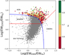 |
Fig. 1. Blue diagram (Lamareille 2010) for the VIMOS sample. Diamonds represent Type II AGN; they are colour-coded according to their redshift. VIMOS galaxies with reliable emission line measurements are shown as grey dots. The blue curve shows the separations between star-forming galaxies and AGN (Eq. (1)), the red dashed line between AGN and LINERs (Eq. (2)), the red solid line between star-forming galaxies and SF/AGN (Eq. (3)). |
The boundary used to distinguish between the Type II AGN and the LINERS regions (shown as red dashed line in Fig. 1) is
![Mathematical equation: $$ \begin{aligned} \log \frac{\mathrm{[OIII]}}{\mathrm{H\beta }} = 0.95 \times \log \frac{\mathrm{[OII]}}{\mathrm{H\beta }} - 0.4, \end{aligned} $$](/articles/aa/full_html/2022/03/aa41072-21/aa41072-21-eq2.gif) (2)
(2)
and the region where SFGs are mixed with AGN (shown as the red solid line in Fig. 1) is given by
![Mathematical equation: $$ \begin{aligned} \log \frac{\mathrm{[OIII]}}{\mathrm{H\beta }} > 0.3. \end{aligned} $$](/articles/aa/full_html/2022/03/aa41072-21/aa41072-21-eq3.gif) (3)
(3)
Given the wavelength distance between [OIII] and Hβ on the one hand, and [OII] doublet lines on the other, these line ratios are sensitive to reddening. Lamareille (2010) demonstrate that the use of equivalent widths instead of line fluxes minimizes this problem, even if it does not eliminate it completely. We thus use EW ratios instead of flux ratios to minimize the effect of reddening.
In Fig. 1 the blue diagram for the VIMOS sample is shown. Our selection of Type II AGN includes 812 objects.
3.3. Ancillary data
In order to carry out our study, we need to estimate galaxy properties such as stellar masses and star formation rates for the VIMOS AGN sample. The study of broad-band spectral energy distribution (SED) is the most commonly adopted method to derive galaxy properties. To estimate the selected AGN stellar mass we collect all available photometric data and fit them with galaxy+AGN templates.
3.3.1. VIPERS photometry
The VIPERS sample has been selected from the W1 and W4 fields of the CFHTLS, which provides magnitudes in the u * ,g, r, i, z photometric bands down to i < 22.5, corrected for Galaxy extinction derived from the Schlegel dust maps (Guzzo et al. 2014; Moutard et al. 2016). The following additional photometric data are available for a subset of sources:
-
NIR observations are available for 98% of the AGN sample in the Ks band in the W1 and W4 fields and in the Kvideo band in the W1 field (Moutard et al. 2016);
-
The VIPERS survey is also covered by GALEX observations in the far-UV (FUV) and near-UV (NUV) bands for 17% of the AGN sample (Moutard et al. 2016);
-
MIR photometry is available for 13% of the AGN targets with Spitzer, from the Spitzer Wide-area Infrared Extragalactic survey (SWIRE) observations in the XMM-LSS field (Lonsdale et al. 2004)
-
Photometric information in the WISE all-sky passbands is also available for 18% of the AGN targets (Wright et al. 2010, VIPERS team).
3.3.2. VVDS photometry
All the VVDS fields have been observed in the B, V, R, and I filters as part of the VIRMOS Deep Imaging Survey (McCracken et al. 2003; Le Fèvre et al. 2004a) with the CFH12K imager at CFHT. The following additional photometric data are available:
-
u * ,g′,r′,i′,z′ photometry from the Canada-France-Hawaii Telescope Legacy Survey (CFHTLS, Cuillandre et al. 2012) is available for 43% of the AGN sample and NIR photometric information from WIRcam InfraRed Deep Survey in the J, H, and K bands (Bielby et al. 2012) and from UKIDSS in the J and K filters (Lawrence et al. 2007) for 38% and 44% of the AGN sample, respectively;
-
FUV and NUV photometry with the GALEX satellite (Arnouts et al. 2005) is available for 2% of the AGN sample and MIR data with the Spitzer (SWIRE survey, Lonsdale et al. 2003) for 3% of the sample;
-
Imaging with the Advanced Camera for Surveys Field Channel instrument on board the Hubble Space Telescope is available for 4% of the AGN sample, in four bands B, V, I, and Z (Le Fèvre et al. 2004b).
3.4. SED fitting analysis
We derived stellar masses and SFRs through SED fitting of the available multiwavelength photometry (see Sect. 3.3.1) using the Code Investigating GALaxy Emission (CIGALE; Noll et al. 2009; Boquien et al. 2019, version 2020.0)2.
CIGALE provides a multi-component SED fit that includes multiple stellar components (old, and young), dust and interstellar medium (ISM) radiation, and AGN emission. The different components are linked to balance the absorbed radiation at UV–optical wavelengths with that re-emitted in the far-infrared (FIR).
The components used for the fitting procedure are (i) the stellar emission, which dominates the wavelength range 0.3−5 μm; (ii) the emission by the cold dust, which is heated by the star formation and dominates the FIR; and (iii) the AGN emission, coming from the accretion disc, peaking at UV–optical wavelengths and reprocessed by the dusty torus in the MIR. In the fitting procedure we fixed the redshift at the value derived from the [OIII] emission line (see Sect. 3). The models adopted for the SED fitting are the following.
For the stellar models we adopted a delayed star formation history (SFH), τ-model, with varying e-folding time and main stellar population ages, defined as
 (4)
(4)
where τ is the e-folding time of the star formation. The SFH is convolved with the stellar library of Bruzual & Charlot (2003) assuming the Chabrier initial mass function (IMF). The metallicity is fixed to solar value, 0.02. We set the separation between the young and old stellar populations to 10 Myr. Dust extinction is modelled by assuming the Calzetti et al. (2000) law. We use the colour-excess E(B − V)* in the range of values shown in Table 1. We assume that old stars have a lower extinction compared to the young stellar populations by a factor of 0.44 (Calzetti et al. 2000).
CIGALE parameters used for the SED fitting.
We adopted the Dale et al. (2014) templates to model the reprocessed emission in the IR from the dust heated by stellar radiation. These templates also include the contribution from the dust heated by AGN. We used them without the AGN contribution, which is set equal to 0 since it is defined separately with the Fritz et al. (2006) templates. The models represent emission from dust which is exposed to different ranges of radiation field intensity and the templates are combined to model the total dust emission with the relative contribution given by a power-law distribution dMdust ∝ U−αdU, with Mdust the dust mass heated by a radiation field and U the radiation field intensity. The free parameter α slope was allowed to vary in the range listed in Table 1.
To parametrize the AGN emission component, we used the models from Fritz et al. (2006), which assume isotropic emission from the central AGN and emission from the dusty torus. The law describing the dust density within the torus is variable along the radial and polar coordinates
 (5)
(5)
with α proportional to the equatorial optical depth at 9.7 μm (τ9.7), and β and γ related to the radial and angular coordinates, respectively. We fixed the parameters β, γ, and θ to parametrize the dust distribution within the torus, according to the values reported in Table 1. The geometry of the torus is described by using the ratio of the outer to the inner radii of the torus, Rmax/Rmin, and the opening angle of the torus, θ. We chose typical values, such as those found in Fritz et al. (2006), and by fixing these parameters we avoided degeneracies in the templates. It is possible to provide a range of inclination angles between the line of sight of the observer and the torus equatorial plane, ψ, with values ranging from 0 for Type II up to 90 for Type I AGN. Another important parameter is the fractional contribution of the AGN emission to the total IR luminosity, fracAGN. We set a wide range of values to account for the possibility that the AGN contribution to the IR luminosity is very low, 5%, up to 95% of the total contribution.
The photometric data are fitted with the models and the physical properties are then estimated through the analysis of the likelihood distribution. In Fig. 2 the distribution of stellar masses for AGN Type II is shown for different redshift bins. We probed stellar masses, Log (Mstellar/M⊙), in the range ∼8−12, with a median (mean) value of 9.5 (10.2).
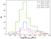 |
Fig. 2. Stellar mass distribution of the Type II AGN host galaxies for the VIMOS sample in different redshift ranges. |
The reliability of the computed host galaxies stellar mass values from the SED fitting analysis can be assessed through the analysis of a mock catalogue. The basic idea is to compare the stellar masses of the mock catalogue (true values), which are known exactly, to the values estimated from the analysis of the likelihood distribution. We used an option included in CIGALE to build a mock catalogue, based on the best-fit model for each object, as derived in Sect. 3.4. A detailed description of the mock analysis can be found in Giovannoli et al. (2011). Briefly, the best-fit SED model of each object is modified by adding a random Gaussian-distributed error to each flux measured in the photometric bands of the dataset, with the same standard deviation as the observed uncertainty in each band. The mock catalogue is then analysed in the same way as the real observations. Figure 3 shows the comparison between the stellar masses derived from the mock analysis and the values estimated for the real sample of Type II AGN. The estimated and true values are closely correlated, indicating that the stellar mass parameter can be consistently constrained, with a Pearson’s correlation coefficient for linear regression of ∼0.98.
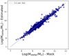 |
Fig. 3. Comparison between the true value of the stellar mass as derived from the mock analysis and the value estimated by SED fitting. The grey dashed line indicates the 1:1 relation between the parameters. |
3.5. Star formation rate
It would also be possible to derive the SFR from the SED decomposition; however, a lack of FIR coverage prevents us from retrieving a reliable estimate of the SFR from the SED (see Ciesla et al. 2015). An alternative SFR indicator is the [OII]λ3726+3728 doublet line. The [OII] emission line is commonly used to measure SFR in star-forming galaxies (e.g. Kennicutt 1998; Hopkins et al. 2003; Kewley et al. 2004), even though it suffers from dust extinction, as it is known to be strongly excited by star formation. For galaxies with an active nucleus, lines of low ionization potential such as [OII] could be excited by both SF and AGN activity; however, it has been observed that the [OII] is mainly produced by star formation (e.g. Ho 2005; Zhuang & Ho 2019).
As discussed in Silverman et al. (2009), the [OII]/[OIII] flux ratio decreases with increasing [OIII] luminosities, and the slope that describes this relation is flatter for Type II AGN than for Type I AGN (see Fig. 4). This difference is explained by an additional contribution to the [OII] flux in Type II AGN due to ongoing star formation. Previously, Kim et al. (2006) explained the enhanced [OII]/[OIII] ratios for Type II Quasars from Zakamska et al. (2003) (median value of [OII]/[OIII] = −0.12) as being due to a more prevalent star formation in Type II AGN. In Fig. 4 we show the [OII]/[OIII] luminosity ratio as a function of [OIII] luminosity for the VIMOS sample. The median value of the [OII]/[OIII] ratio is −0.14, consistent with the Zakamska et al. sample. We note that the line luminosities are not corrected for extinction; therefore, the line ratios can be considered lower limits. We also plot the best-fit linear relation for SDSS Type I (dashed line) and Type II (solid line) sources as reported in Silverman et al. (2009). Type II AGN in the VIMOS sample exhibit a similar slope to the SDSS Type II AGN and have slightly enhanced [OII]/[OIII] ratios compared to the SDSS sample. This finding further justifies the use of this line as a SFR indicator (e.g. Silverman et al. 2009; Kim et al. 2006).
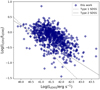 |
Fig. 4. [OII]/[OIII] luminosity ratio as a function of [OIII] luminosity for the VIMOS Type II AGN. The dashed and solid lines represent the best-fit relation for SDSS Type I and Type II AGN at z < 0.3, respectively. |
Assuming that high ionization lines such as [OIII] are mainly powered by AGN activity (e.g. Kauffmann et al. 2003c), we adopted this line to remove the AGN contribution from the [OII] line. Recently, Zhuang & Ho (2019) found a fairly constant [OII]/[OIII] ∼ 0.10 for the Type II AGN contribution according to a set of photoionization models; we therefore subtracted 10% of the [OIII] luminosity from the [OII] line. We then derived the SFR by using the calibration from Kewley et al. (2004) (rescaled by a factor of 1.7 to account for the different IMF used),
![Mathematical equation: $$ \begin{aligned} \mathrm{SFR_{[OII]}} = 6.58 \pm 1.65 \times 10^{-42} (L_{\rm [OII]} - 0.109\,L_{\rm [OIII]})\,(M_{\odot }\,\mathrm{yr^{-1}}), \end{aligned} $$](/articles/aa/full_html/2022/03/aa41072-21/aa41072-21-eq6.gif) (6)
(6)
where L[OII] and L[OIII] are in units of erg s−1. We probed SFR in the range 0.01−38 M⊙ yr−1, with a median (mean) value of 0.8 (1.3) M⊙ yr−1.
4. Results
4.1. SFR-stellar mass plane
In Fig. 5 we show the SFR-stellar mass relation for the Type II AGN host galaxies of the VIMOS sample. We indicate the star-forming MS relation at z = 0.7, the mean redshift of our sample, from Schreiber et al. (2015) (solid curve) along with the scatter (0.4 dex, dashed lines). We rescaled both the SFR and stellar masses of Schreiber et al. (2015) by a factor of 1.7 to account for the different IMF used (Salpeter vs. Chabrier). The bulk of the VIMOS sample populates the MS region, with a fraction of AGN host galaxies on and off the MS.
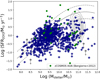 |
Fig. 5. Star formation rate as a function of stellar mass (Mstellar) for the VIMOS sample (blue diamonds). The solid line represents the star-forming main sequence found by Schreiber et al. (2015), and the dashed lines give the scatter of 0.4 dex. Upper limits are shown as grey diamonds. The optically selected Type II AGN from zCOSMOS survey found by Bongiorno et al. (2012) and from BOSS DR12 are shown as green circles and grey contours, respectively. |
At high stellar masses (> 1010 M⊙) almost all sources are below the MS (see Fig. 5). Overall, Type II host galaxies show a broader distribution of SFR than star-forming MS galaxies, consistent with previous studies (e.g. Mullaney et al. 2015).
As discussed in Bongiorno et al. (2012), optically selected Type II sources from the zCOSMOS-bright survey show properties similar to the VIMOS sample. This is not surprising since the two surveys cover similar volumes and depths. We add this sample in Fig. 5 as green circles. These sources are selected through the blue diagram in the redshift range 0.50 < z < 0.92, with stellar masses and SFRs derived through SED fitting analysis. In terms of stellar masses and SFR, they span the same range as the VIMOS Type II AGN galaxies, and for these sources the MS locus at high stellar masses remains underpopulated for Type II AGN host galaxies with respect to what is found for star-forming galaxies, suggesting that the distribution could be different with respect to non-AGN galaxies.
We investigate whether a fraction of Type II AGN can be missed by the adopted selection criteria. One possibility is that this missing fraction could reside in the composite locus of SF-Type II AGN. A high level of star formation can produce an enhancement in the Hβ flux, moving a Type II AGN down to the composite locus in the blue diagram plane. We therefore investigated the host galaxies properties of the composite sources (as defined by the blue diagram) in the VIPERS sample. We collected their SED-based stellar masses and measured the SFR using the [OII]λ3727 emission line. We found that the composite galaxies actually exhibit stellar masses < 1010 M⊙ and SFRs slightly enhanced with respect to those observed for Type II AGN in a similar mass range. This indicates that the missing fraction of Type II AGN is not classified as composite.
We also compare the VIMOS sample with the DR12 BOSS sample of Type II AGN (Thomas et al. 2013). Specifically, we used the galaxy properties (i.e. emission line measurements, BPT classification, and stellar masses) derived by the Portsmouth Group for the BOSS DR12 (Thomas et al. 2013). They applied the blue diagram criterion to select a Type II AGN sample at redshift 0.5 < z < 0.9. We restricted our analysis to those galaxies with [OIII], [OII], and Hβ flux detection over 2σ (as defined by the amplitude-to-noise ratio parameter). For consistency with the VIMOS sample, we measured SFRs of the Type II AGN host galaxies from the BOSS DR12 using the [OII]λ3727+3729 emission line fluxes, subtracting off the AGN contribution by using the [OIII]λ5007 line flux (see Eq. (6)). Stellar masses are calculated by the Portsmouth team from the best-fit SED (Maraston et al. 2013). They used two types of templates to derive stellar masses, i.e. passively evolving and star-forming models, based on the galaxy types expected according to the BOSS colour cut. As presented in Thomas et al. (2013), BOSS Type II AGN preferentially show a g − r colour (strongly dependent on the star formation history of galaxies) between that observed for luminous red and star-forming galaxies. Here we used stellar masses from the star-forming model, and note that stellar masses could be underestimated.
A dust extinction effect could still play a role. In the case of a highly star-forming galaxy (and high stellar mass) with an AGN, the Hβ emission line could remain undetected due to attenuation by dust, and hence the galaxy would be excluded from our sample selection. This would result in a missing fraction of galaxies with high stellar mass. We therefore compare our sample with the Type II AGN from the BOSS survey. The bulk of Type II AGN is preferentially found in host galaxies with stellar mass > 1010 M⊙, due to the BOSS selection colour cut favouring the most massive galaxies and 17% of Type II AGN from the BOSS survey occupies the locus of MS and starburst. Despite the slightly enhanced statistics than that probed by the VIMOS targets, we can conclude they are overall consistent, considering the small area covered by VIPERS and VVDS surveys (24 deg2 for VIPERS, and 8.7 deg2, 0.74 deg2, and 512 arcmin2 for VVDS-Wide, Deep, and Ultra Deep, respectively) with respect to the BOSS survey (∼10 000 deg2).
4.2. Correlation between SFR offset from the main sequence and AGN luminosity
Feedback from AGN could be responsible for the quenching of star formation in massive galaxies, with increasing AGN efficiency in driving outflows at increasing AGN luminosity (e.g. Menci et al. 2008; Faucher-Giguère & Quataert 2012; Hopkins et al. 2016).
To test this point, we examined the relationship between the SFR offset from MS and the AGN power. In Fig. 6 we show the relative offset of the SFR from the MS relation of Schreiber et al. (2015) as a function of [OIII] luminosity, which can be considered to be a proxy of AGN power. VIMOS Type II AGN host galaxies show different properties in terms of star formation with a clear dependence on stellar mass, forming two distinct groups of AGN in this diagram: at a fixed AGN power, Type II AGN host galaxies at Mstellar < 1010 M⊙ show higher star formation activity than more massive galaxies. To define the boundary of this bimodality, we divided our targets into five subsamples with different AGN power (indicated in Fig. 6, left panel). In each luminosity bin, we used the Gaussian kernel density estimation (KDE) to estimate the probability density function of the SFR offset and derive the separation between the two subsamples (see right panel of Fig. 6). We proceeded as follows: (i) we fit two Gaussians to reproduce the bimodality of KDE functions; (ii) we derive the intersection point of the two best-fit Gaussians in each bin; and (iii) we perform a linear regression on the intersection points. The best-fit line to these points (i.e. 0.54 × Log (L[OIII]/erg s−1)−23.22) is shown in Fig. 6, left panel, as a black solid line.
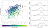 |
Fig. 6. SFR offset from the MS (parametrized as SFR[OII]/SFRMS) and its probability density function in bins of [OIII] luminosity for the VIMOS sample. Left panel: SFR offset is shown as a function of [OIII] luminosity (proxy of AGN power) with full diamonds, colour-coded according to the stellar mass. Circles and stars represent median values of the SFR offset derived using [OII]-based and SED-based SFRs, respectively, for the subset of sources above the black diagonal line (brown) and for those below (orange) in five bins of [OIII] luminosity (see main text for details). The five bins of [OIII] luminosity are given by the black horizontal segments. The horizontal dashed lines delimit the locus of the MS ± 0.4 dex. Right panel: probability density function of the SFR offset (black solid curves) in the five [OIII] luminosity bins in the left panel, with superimposed the best-fit double Gaussian components (black dashed curves) which reproduce the observed bimodality. The intersection points of the two Gaussians in the five luminosity bins are represented as upside down triangles in the left panel (see Sect. 4.2). |
Above the boundary line, 64% of the VIMOS subsample occupies the same region as the star-forming (i.e. log(SFR[OII]/SFRMS) within ±0.4 dex) and starburst galaxies (i.e. log(SFR[OII]/SFRMS) > 0.4), with stellar mass mostly below 1010 M⊙, and the remaining 36% have SFRs below the bulk of the MS galaxies but above the quiescent locus (sub-MS, −1.3 < log(SFR[OII]/SFRMS) < −0.4). Hereafter, we refer to this subsample as high-SF Type II AGN. Instead, below the line threshold the diagram is occupied by massive targets along the MS (3%), 51% in the sub-MS and 46% in the quiescent regime (i.e. log(SFR[OII]/SFRMS) < −1.3, e.g. Aird et al. 2019). Hereafter, we refer to this subsample as low-SF Type II AGN.
Since our sample does not have Hα and Hβ within the observed spectral window, we could not compute the Balmer decrement, and as a consequence did not correct the line luminosities for extinction. We explored the possible effect the extinction could have on the presence of the two populations. Rosa-González et al. (2002) show that the excess in the [OII]-based and UV-based SFR estimates is mainly due to an overestimation of the extinction resulting from the effect of underlying stellar Balmer absorptions in the measured emission line fluxes. Therefore they constructed unbiased SFR estimators, which statistically include the effect of underlying stellar Balmer absorptions in the measured emission line fluxes.
Kewley et al. (2004) found a strong correlation between the intrinsic [OII] luminosity and the colour excess for the galaxies in Nearby Field Galaxies Survey, deriving a direct relation between intrinsic and observed [OII] luminosity, although they note that the relation should not be blindly applied to other galaxies. We have tested what happens to the distribution shown in Fig. 6 applying either the extinction correction by Kewley et al. (2004) given in Eq. (18) or the recipe by Rosa-González et al. (2002). In both cases we still find the observed separation between low- and high-SF AGN, and we can therefore conclude that the bimodality does not depend on the extinction.
In the following we investigate whether the offset from the MS is related to the AGN power by comparing it with the [OIII] luminosity. In Fig. 6 we show the median Log (SFR/SFRMS) in bins of [OIII] luminosity of the high- and low-SF subsamples (brown and orange circles respectively, where the errors bars indicate the 25th and 75th percentiles). We find a correlation between the relative offset of the SFR from the MS and the AGN power for both populations: at increasing AGN luminosities Type II AGN hosts tend to have higher SFR. As a positive correlation exists between the [OII] and [OIII] luminosity, as a counter-check we performed the same analysis using the SFR derived from the SED fitting, obtaining similar results but with a shallower slope, thus confirming the reliability of our findings (see stars in Fig. 6).
Previous works examined the connection between the SFR and AGN activity, with controversial results claiming strong to weak or absent relations (e.g. Azadi et al. 2015; Chen et al. 2013; Stanley et al. 2015, 2017; Harrison et al. 2012). The origin of these discrepancies could be related to sample selection effects, methods of estimating the SFR and the AGN luminosity, as well as the number statistics of the sample (e.g. Harrison et al. 2012). Harrison et al. (2012) reported that the SFR of z = 1 − 3 AGN is independent of X-ray luminosity, used as an indicator of AGN activity. This result is in contrast with that found by Page et al. (2012) and the authors suggest that the poor statistics is at least partially responsible for the disagreement at high luminosity between their work and that of Page et al. (2012). Stanley et al. (2015) used 2000 X-ray detected AGN to investigate the SFR and AGN luminosity relation, in the redshift range 0.2 < z < 2.5 and with X-ray luminosity 1042 < L2 − 8 kev < 1045.5 erg s−1. They used infrared SED decomposition (AGN+star formation components) to derive IR-based SFR and X-ray luminosity as a probe of AGN power, founding a broadly flat SFR-AGN luminosity relation at all redshifts and all the AGN luminosities investigated. They argue that the flat observed relation is probably due to short timescale variations in AGN luminosity (probed by X-ray luminosity), which can wash out the long-term relationship between SFR and AGN activity. Masoura et al. (2021) found a positive correlation between the MS offset and the X-ray luminosity of a sample of X-ray selected Type II AGN at 0.03 < z < 3.5. Zhuang & Ho (2020) analysed a sample of 5800 Type I and 7600 Type II AGN at z < 0.35 to study the star formation activity based on [OII] and [OIII] emission lines, finding a tight linear correlation between AGN luminosity (probed by [OIII] emission) and SFR. The [OIII] AGN indicator probes the AGN activity on longer timescales than X-ray luminosity, which traces the instantaneous AGN strength, and therefore the use of [OIII] may result in a stronger correlation between SFR and AGN luminosity.
The positive correlation found for SFR and AGN activity support the idea that the AGN and the star formation activity in the host galaxy are sustained by a common fuelling mechanism, the large amounts of cold gas, and that the growths of the stellar mass and of the SMBH proceed concurrently (e.g. Silverman et al. 2009; Santini et al. 2012).
However at high stellar masses Type II AGN host galaxies show systematically lower SFR values. This could indicate that the process of AGN growth is linked to the process of star formation in AGN host galaxies (e.g. Matsuoka et al. 2015; Mullaney et al. 2015; Shimizu et al. 2015). The AGN could work against star formation, decreasing the gas reservoir in several ways, such as mechanical heating and powerful outflows, moving the host galaxies of Type II AGN down to the quiescent locus in the SFR–Mstellar plane.
4.3. Low-SF and high-SF Type II AGN properties
4.3.1. [OIII] line shape
About 50% of our Type II AGN host galaxies are located below the MS. Their lower-than-expected SFRs might be evidence of ongoing quenching. Powerful AGN radiation is often invoked as one of the main mechanisms that halt star formation by ejecting the gas necessary to fuel it. The ejected gas can be traced at all scales, and in various gas components: blueshifted absorption lines from the accretion disc (i.e. ultra-fast outflows; e.g. Tombesi et al. 2010), blueshifted emission line components produced by ionized gas in the BLR (e.g. CIV; Vietri et al. 2020 and references therein) and NLR (e.g. [OIII]; Harrison et al. 2016), and as blueshifted lines produced by outflowing cold molecular gas on galactic scales (e.g. CO; Polletta et al. 2011, and many others). Here we investigate whether we find any evidence of AGN-driven outflowing gas by analysing the profile of the [OIII] emission line. Each population (as defined in Sect. 4.2) is divided into [OIII] luminosity bins as done in Sect. 4.1.
We performed a median spectral stack, by using the IRAF task scombine, resampling spectra to a rest-frame wavelength grid from 3520 Å with a step size of 4.29 Å, corresponding to the wavelength resolution at redshift 0.7, the mean redshift of the sources studied in this paper. We also normalized each spectrum to the continuum from 4500 Å up to 4600 Å, where the spectrum is free of strong emission and absorption lines.
We analysed the line profile of the [OIII]λ4959,5007 doublet, Hβ and [OII] doublet by fitting the lines with two models, considering a single and a double Gaussian to search for a possible second broad and shifted component, indicative of the presence of outflow. We used the same constraints as discussed in Sect. 3. We adopted the double-Gaussian model as best fit when it satisfies the Bayesian Information Criterion (BIC, Schwarz 1978), which uses differences in χ2 that penalize models with more free parameters. For both models we estimated the BIC defined as χ2 + k ln(N), with N the number of data points and k the number of free parameters of the model. For each stacked spectrum we derived the ΔBIC = BIC1–BIC2, where BIC1 and BIC2 are derived from the models with one and two Gaussian profiles, respectively. We favoured the fit with a single-Gaussian profile when ΔBIC < 10.
In Fig. 7 we compared the spectral properties of the Hβ and [OIII] doublet lines in each [OIII] luminosity bin and for each subsample. In all but the high-luminosity bin of the low-SF Type II AGN hosts, the [OIII] line appears to be symmetrical, as the preferred single-Gaussian model and visual inspection suggest.
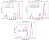 |
Fig. 7. Comparison of the stacked spectra, in the Hβ–[OIII] doublet lines wavelength range, in bins of [OIII]λ5007 luminosity above (left) and below (right) the line threshold, as defined in Sect. 4.2 (lower panel). Stacked spectrum in the [OIII] luminosity bin Log (L[OIII]/erg s−1) > 42.5 of the low-SF Type II AGN with superimposed the 1σ uncertainties estimated through a bootstrap resampling technique and the best-fitting one-component Gaussian curve (black dashed line). The inset shows the best-fit double-Gaussian model (magenta curve) and its line decomposition (green and blue Gaussian profiles refer to the narrow and broad best-fit components). |
Only in the highest luminosity bin (Log (L[OIII]/erg s−1) > 42.5) of the low-SF population, does there seem to be a hint of asymmetry in the [OIII] line profile. Figure 7 (bottom panel) shows the spectrum (magenta line) and the best-fitting single-component Gaussian (black dashed line). To rule out that such an excess is compatible with errors, we estimated the uncertainties on the stack through a bootstrap resampling technique, creating 1000 realizations of the AGN stack spectra with replacement, and derived the 1σ uncertainties from the 84th and 16th percentiles of the bootstrap distribution, shown as the grey area in Fig. 7 (bottom panel). In the fitting a double-Gaussian model is preferred, with a centroid of the second component nearly at systemic redshift and a FWHM of 1260 km s−1, after correcting for instrumental broadening (see inset in Fig. 7, bottom panel).
This finding is in agreement with previous results that reported an increasing outflow component at increasing luminosity (e.g. Mullaney et al. 2013). The presence of outflowing gas in galaxies with stellar mass > 1010 M⊙ and their position in SFR-stellar mass plane is qualitatively consistent with the evolutionary scenario, where the AGN is capable of driving outflows that could regulate the star formation and the baryonic content of galaxies.
The line profile analysis indicates the presence of disturbed kinematics only in the high-luminosity bin of the low-SF sample. We do not find a similar result for the high-SF sample at the highest luminosity bin. This could be either due to the absence of outflow in galaxies with stellar mass < 1010 M⊙ or, considering the unified model, to the fact that the outflowing material should emerge in a direction perpendicular to the plane of the obscuring torus (i.e. to our line of sight), resulting in a small projected velocity of the outflow and/or in a symmetric line profile, which can explain the symmetric profiles found for most of the stacked VIMOS sample (see Mullaney et al. 2013; Harrison et al. 2012). If the outflow signature is unresolved, it could be that the outflows are not quenching the star formation in these systems or that the timescale is actually longer than the stage at which these objects are seen.
Higher resolution spectroscopy becomes necessary to characterize subtle spectral features and distinguish between gravitational and non-gravitational motions. This would provide a deep insight on the AGN feedback in these systems.
4.3.2. Black hole masses and Eddington ratios
Previous studies have shown that there is a correlation among strong blue wings, the large FWHM of line profiles originating in the NLR, and the Eddington ratio, which describes the accretion mechanism of an AGN (e.g. Woo et al. 2016). The Eddington ratio is defined as
 (7)
(7)
where LEdd(=1.27 × 1038 MBH, with MBH indicating the BH mass) is the limit at which the outward radiation pressure from the accreting matter balances the inward gravitational pressure exerted by the BH, and LBol is the bolometric luminosity.
Black hole masses for Type I AGN are usually estimated indirectly by using the virial theorem, which links the BH mass to the BLR radius and the gas velocity dispersion. Considering the Hα emission line, the single-epoch relation can be written as (Baron & Ménard 2019)
 (8)
(8)
with ϵ the virial shape factor, λLλ5100 the monochromatic AGN luminosity at 5100 Å, and FWHM the BLR component of the Hα emission line.
However, Type II AGN are viewed edge-on, preventing us from seeing the BLR, which is obscured by the presence of a dusty torus. Therefore, in Type II AGN BH masses cannot be estimated by using the single-epoch mass determination, which requires the view of BLR clouds. Indirect methods can be used as the well-known correlations between the BH mass and host galaxy bulge stellar mass or stellar velocity dispersion. However, these relations are established for local inactive galaxies. Recently, Baron & Ménard (2019) have found a correlation between the narrow L([OIII])/L(Hβ) line ratio and the width of the Hα BLR component, linking the kinematics of the BLR clouds to the ionization state of the NLR as follows:
![Mathematical equation: $$ \begin{aligned} \mathrm{log} \frac{L_{\rm [OIII]}^\mathrm{narrow}}{L_{\rm H\beta }^\mathrm{narrow}} = 0.58 \pm 0.07 \times \log \frac{FWHM _{\rm H_{\alpha }}^\mathrm{BLR}}{\mathrm{km\,s^{-1}}} -1.38 \pm 0.38. \end{aligned} $$](/articles/aa/full_html/2022/03/aa41072-21/aa41072-21-eq10.gif) (9)
(9)
This power-law dependence holds for AGN-dominated systems with log([OIII]/Hβ) > 0.55. We therefore derive the BLR Hα FWHM component for the 79% of our targets, exhibiting log([OIII]/Hβ) > 0.55. For the continuum luminosity we rely on the relation found by Baron & Ménard (2019)
 (10)
(10)
and on Heckman et al. (2004) for the bolometric luminosity, inferred from the [OIII] luminosity with no correction for dust extinction and applying a bolometric correction of 3500.
We derive BH masses in the range ∼107 − 10 M⊙ and λEdd ∼ 10−3 − 0.5, with a median value of ∼0.08, consistent with what is found in other AGN samples (e.g. Lamastra et al. 2009) We now explore if there is an indication of a variation in BH mass and Eddington ratio distribution between the Type II AGN groups in Fig. 8. Despite the wide range spanned, differences between BH mass and λEdd distributions are discernible. The median values for each parameter are shown as vertical lines in corresponding colours and line styles. The median value of λEdd derived for the high-SF galaxies is slightly higher than that derived for low-SF galaxies. Furthermore, these galaxies are less massive and have in general lower BH mass than low-SF galaxies. On the contrary, this latter galaxy sample shows larger values of BH mass, the distribution of which points towards higher BH mass values, as shown by the MBH distribution in Fig. 8.
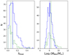 |
Fig. 8. Eddington ratio (left) and black hole mass (right) distributions of Type II AGN divided into two subsamples, according to the classification of their host galaxies as high-SF (blue) and low-SF (green). The solid and dashed lines represent the median value of the parameters. |
To assess the difference between the distributions, we compute the Kolmogorov-Smirnov (K-S) test for the λEdd and BH mass distributions of the two groups of Type II AGN. The null-hypothesis is that the two samples are drawn from the same parent population. The K-S test was performed by using the python routine scipy.stat.ks_2samp. For the λEdd distributions we compute a statistic of 0.3 and p-value = 2.6 × 10⁻⁸ and for BH mass distributions a statistic of 0.2 and p-value = 4.5 × 10⁻⁶. The very low probability value excludes that the two groups of Type II AGN are drawn from the same parent population, suggesting that the difference between these groups also relates to the AGN activity.
It is instructive to compare these findings with what is found in the local Universe. Kauffmann & Heckman (2009) examined the dependence of the distribution of the Eddington ratio on the star formation history of SDSS Type II AGN. They found that the Eddington ratio distributions can be different for actively star-forming and passive host galaxies. Specifically, they divided these two populations according to the break index D(4000) (Balogh et al. 1999), a useful diagnostic of the recent star formation history in these systems. The star-forming host galaxies show a log-normal distribution of Eddington ratios peaking at a few percent of Eddington luminosity, independent of black hole masses. This regime dominates the growth of BH with mass < 108 M⊙, while the passive galaxies (D4000 > 1.7) show a power-law distribution of Eddington ratios with its amplitude decreasing with increasing black hole mass. This regime dominates the growth of BH with mass > 108 M⊙. This finding is in line with our evidence of different accretion rates distribution for high- and low-SF Type II AGN host galaxies.
Finally, although the estimated Eddington ratios have large uncertainties, we did not find a clear dependence of the broadening of the [OIII] line with the Eddington ratio since the only evidence of outflowing gas is found in the [OIII]-luminous low-SF galaxies, which are accreting at ∼5% of the Eddington luminosity, a lower rate than that of the high-SF Type II AGN subsample, which show average Eddington ratios of ∼0.10. This could be interpreted as a final decay phase of the AGN activity in the [OIII]-luminous low-SF galaxies, where the outflowing gas persists but the AGN feeding mechanism is fading as is the star formation activity, likely due to AGN feedback.
5. Summary and conclusions
In this paper we have used the VVDS and VIPERS optical spectroscopic surveys, carried out using the VIMOS spectrograph, to select and investigate the properties of those galaxies hosting an AGN at redshift 0.5 < z < 0.9. We have analysed the emission line properties of the [OIII] and [OII] doublets, and the Hβ, and adopted the blue diagram of Lamareille (2010) to distinguish Type II AGN from star-forming galaxies and LINERS through emission line ratios [OIII]/Hβ versus [OII]/Hβ.
Our main findings can be summarized as follows:
(i) The masses of the host galaxies range from 108 to 1012 M⊙, with a median value of 109.5 M⊙ and span a SFR range of 0.01−38 M⊙ yr−1. The VIMOS sample with stellar mass < 1010 M⊙ mostly resides on the star-forming MS locus, as defined by Schreiber et al. (2015), with a fraction of sources (∼20%) between the MS and quiescent region having stellar mass > 1010 M⊙, indicating reduced level of star formation.
(ii) We find a bimodality in the SFR MS offset-AGN power plane (probed by the [OIII] luminosity), and ascribe them to two different populations in the VIMOS sample. We divide our Type II AGN sample into two groups according to the properties of their host galaxies, the high-SF group with stellar mass < 1010 M⊙, occupying the star-forming MS region, and the low-SF group with levels of star formation between the MS and quiescent locus and even lower, and stellar mass greater than 1010 M⊙. For both populations a positive correlation exists between the SFR offset from the MS and the AGN power, which could reflect the available amount of gas that both triggers star formation and fuels the AGN activity. Despite this positive correlation, a lower level of star formation rates are found in low-SF Type II galaxies.
(iii) AGN feedback may be responsible for reducing the supply of cold gas in host galaxies at least for AGN luminous systems. For the [OIII]-luminous low-SF galaxies we found a hint of outflowing gas, as probed by the asymmetric [OIII] line profile, which could be connected with the low SFR content found, possibly due to the effect of AGN acting on the ISM, expelling a certain amount of gas. These massive low-SF galaxies seem to be at their final AGN stage, as indicated by their average Eddington ratio value (∼5% of Eddington luminosity).
The spectral analysis was performed with the python routine scipy.optimize.curve_fit.
CIGALE can also handle upper limits.
Acknowledgments
We thank the anonymous referee for the helpful comments. GV acknowledges financial support from Premiale 2015 MITic (PI: B. Garilli). AP and KM acknowledge support from the Polish National Science Centre under grants: UMO-2018/30/M/ST9/00757 and UMO-2018/30/E/ST9/00082. GM acknowledges support from ST/P006744/1. The results published have been funded by the European Union’s Horizon 2020 research and innovation programme under the Maria Skłodowska-Curie (grant agreement No 754510), the National Science Centre of Poland (grant UMO-2016/23/N/ST9/02963) and by the Spanish Ministry of Science and Innovation through Juan de la Cierva-formacion program (reference FJC2018-038792-I). Based on observations made with ESO Telescopes at the La Silla or Paranal Observatories under programme ID(s) 182.A-0886(H), 182.A-0886(N), 182.A-0886(K), 182.A-0886(R), 182.A-0886(G), 182.A-0886(C), 182.A-0886(B), 182.A-0886(O), 182.A-0886(P), 182.A-0886(J), 182.A-0886(D), 182.A-0886(I), 182.A-0886(Q), 60.A-9157(B). Based on data obtained with the European Southern Observatory Very Large Telescope, Paranal, Chile, under Large Programmes 070.A-9007 and 177.A-0837.
References
- Aird, J., Coil, A. L., Georgakakis, A., et al. 2015, MNRAS, 451, 1892 [Google Scholar]
- Aird, J., Coil, A. L., & Georgakakis, A. 2019, MNRAS, 484, 4360 [NASA ADS] [CrossRef] [Google Scholar]
- Alexander, D. M., & Hickox, R. C. 2012, New Astron. Rev., 56, 93 [Google Scholar]
- Antonucci, R. 1993, ARA&A, 31, 473 [Google Scholar]
- Arnouts, S., Schiminovich, D., Ilbert, O., et al. 2005, ApJ, 619, L43 [NASA ADS] [CrossRef] [Google Scholar]
- Azadi, M., Aird, J., Coil, A. L., et al. 2015, ApJ, 806, 187 [NASA ADS] [CrossRef] [Google Scholar]
- Baldry, I. K., Glazebrook, K., Brinkmann, J., et al. 2004, ApJ, 600, 681 [Google Scholar]
- Baldwin, J. A., Phillips, M. M., & Terlevich, R. 1981, PASP, 93, 5 [Google Scholar]
- Balogh, M. L., Morris, S. L., Yee, H. K. C., Carlberg, R. G., & Ellingson, E. 1999, ApJ, 527, 54 [Google Scholar]
- Baron, D., & Ménard, B. 2019, MNRAS, 487, 3404 [CrossRef] [Google Scholar]
- Bielby, R., Hudelot, P., McCracken, H. J., et al. 2012, A&A, 545, A23 [NASA ADS] [CrossRef] [EDP Sciences] [Google Scholar]
- Blanton, M. R., Hogg, D. W., Bahcall, N. A., et al. 2003, ApJ, 594, 186 [NASA ADS] [CrossRef] [Google Scholar]
- Bluck, A. F. L., Mendel, J. T., Ellison, S. L., et al. 2014, MNRAS, 441, 599 [NASA ADS] [CrossRef] [Google Scholar]
- Bongiorno, A., Merloni, A., Brusa, M., et al. 2012, MNRAS, 427, 3103 [Google Scholar]
- Boquien, M., Burgarella, D., Roehlly, Y., et al. 2019, A&A, 622, A103 [NASA ADS] [CrossRef] [EDP Sciences] [Google Scholar]
- Bruzual, G., & Charlot, S. 2003, MNRAS, 344, 1000 [NASA ADS] [CrossRef] [Google Scholar]
- Calzetti, D., Armus, L., Bohlin, R. C., et al. 2000, ApJ, 533, 682 [NASA ADS] [CrossRef] [Google Scholar]
- Cappellari, M. 2012, Astrophysics Source Code Library [record ascl:1210.002] [Google Scholar]
- Cattaneo, A., Faber, S. M., Binney, J., et al. 2009, Nature, 460, 213 [NASA ADS] [CrossRef] [Google Scholar]
- Chen, C.-T. J., Hickox, R. C., Alberts, S., et al. 2013, ApJ, 773, 3 [NASA ADS] [CrossRef] [Google Scholar]
- Ciesla, L., Charmandaris, V., Georgakakis, A., et al. 2015, A&A, 576, A10 [NASA ADS] [CrossRef] [EDP Sciences] [Google Scholar]
- Cowie, L. L., Songaila, A., Hu, E. M., & Cohen, J. G. 1996, AJ, 112, 839 [Google Scholar]
- Croton, D. J., Springel, V., White, S. D. M., et al. 2006, MNRAS, 365, 11 [Google Scholar]
- Cuillandre, J. C. J., Withington, K., Hudelot, P., et al. 2012, in Observatory Operations: Strategies, Processes, and Systems IV, eds. A. B. Peck, R. L. Seaman, & F. Comeron, SPIE Conf. Ser., 8448, 84480M [NASA ADS] [CrossRef] [Google Scholar]
- Daddi, E., Dickinson, M., Morrison, G., et al. 2007, ApJ, 670, 156 [NASA ADS] [CrossRef] [Google Scholar]
- Dale, D. A., Helou, G., Magdis, G. E., et al. 2014, ApJ, 784, 83 [Google Scholar]
- Di Matteo, T., Springel, V., & Hernquist, L. 2005, Nature, 433, 604 [NASA ADS] [CrossRef] [Google Scholar]
- Elbaz, D., Daddi, E., Le Borgne, D., et al. 2007, A&A, 468, 33 [NASA ADS] [CrossRef] [EDP Sciences] [Google Scholar]
- Faucher-Giguère, C.-A., & Quataert, E. 2012, MNRAS, 425, 605 [Google Scholar]
- Ferrarese, L., & Merritt, D. 2000, ApJ, 539, L9 [Google Scholar]
- Fritz, J., Franceschini, A., & Hatziminaoglou, E. 2006, MNRAS, 366, 767 [Google Scholar]
- Fritz, A., Scodeggio, M., Ilbert, O., et al. 2014, A&A, 563, A92 [NASA ADS] [CrossRef] [EDP Sciences] [Google Scholar]
- Gabor, J. M., Davé, R., Finlator, K., & Oppenheimer, B. D. 2010, MNRAS, 407, 749 [NASA ADS] [CrossRef] [Google Scholar]
- Gadotti, D. A. 2009, MNRAS, 393, 1531 [Google Scholar]
- Garilli, B., Guzzo, L., Scodeggio, M., et al. 2014, A&A, 562, A23 [NASA ADS] [CrossRef] [EDP Sciences] [Google Scholar]
- Gebhardt, K., Bender, R., Bower, G., et al. 2000, ApJ, 539, L13 [Google Scholar]
- Giovannoli, E., Buat, V., Noll, S., Burgarella, D., & Magnelli, B. 2011, A&A, 525, A150 [NASA ADS] [CrossRef] [EDP Sciences] [Google Scholar]
- Gültekin, K., Richstone, D. O., Gebhardt, K., et al. 2009, ApJ, 698, 198 [Google Scholar]
- Guzzo, L., Scodeggio, M., Garilli, B., et al. 2014, A&A, 566, A108 [NASA ADS] [CrossRef] [EDP Sciences] [Google Scholar]
- Harrison, C. M. 2017, Nat. Astron., 1, 0165 [NASA ADS] [CrossRef] [Google Scholar]
- Harrison, C. M., Alexander, D. M., Swinbank, A. M., et al. 2012, MNRAS, 426, 1073 [NASA ADS] [CrossRef] [Google Scholar]
- Harrison, C. M., Alexander, D. M., Mullaney, J. R., et al. 2016, MNRAS, 456, 1195 [Google Scholar]
- Hasinger, G., Miyaji, T., & Schmidt, M. 2005, A&A, 441, 417 [NASA ADS] [CrossRef] [EDP Sciences] [Google Scholar]
- Heckman, T. M., Kauffmann, G., Brinchmann, J., et al. 2004, ApJ, 613, 109 [Google Scholar]
- Hickox, R. C., Mullaney, J. R., Alexander, D. M., et al. 2014, ApJ, 782, 9 [NASA ADS] [CrossRef] [Google Scholar]
- Ho, L. C. 2005, ApJ, 629, 680 [CrossRef] [Google Scholar]
- Hopkins, A. M., Miller, C. J., Nichol, R. C., et al. 2003, ApJ, 599, 971 [Google Scholar]
- Hopkins, P. F., Richards, G. T., & Hernquist, L. 2007, ApJ, 654, 731 [Google Scholar]
- Hopkins, P. F., Torrey, P., Faucher-Giguère, C.-A., Quataert, E., & Murray, N. 2016, MNRAS, 458, 816 [NASA ADS] [CrossRef] [Google Scholar]
- Kauffmann, G., & Haehnelt, M. 2000, MNRAS, 311, 576 [Google Scholar]
- Kauffmann, G., & Heckman, T. M. 2009, MNRAS, 397, 135 [NASA ADS] [CrossRef] [Google Scholar]
- Kauffmann, G., Heckman, T. M., White, S. D. M., et al. 2003a, MNRAS, 341, 54 [Google Scholar]
- Kauffmann, G., Heckman, T. M., White, S. D. M., et al. 2003b, MNRAS, 341, 33 [Google Scholar]
- Kauffmann, G., Heckman, T. M., Tremonti, C., et al. 2003c, MNRAS, 346, 1055 [Google Scholar]
- Kennicutt, R. C., Jr. 1998, ARA&A, 36, 189 [Google Scholar]
- Kewley, L. J., Geller, M. J., & Jansen, R. A. 2004, AJ, 127, 2002 [Google Scholar]
- Kim, M., Ho, L. C., & Im, M. 2006, ApJ, 642, 702 [NASA ADS] [CrossRef] [Google Scholar]
- Kormendy, J., & Ho, L. C. 2013, ARA&A, 51, 511 [Google Scholar]
- Lamareille, F. 2010, A&A, 509, A53 [CrossRef] [EDP Sciences] [Google Scholar]
- Lamareille, F., Brinchmann, J., Contini, T., et al. 2009, A&A, 495, 53 [NASA ADS] [CrossRef] [EDP Sciences] [Google Scholar]
- Lamastra, A., Bianchi, S., Matt, G., et al. 2009, A&A, 504, 73 [NASA ADS] [CrossRef] [EDP Sciences] [Google Scholar]
- Lanzuisi, G., Delvecchio, I., Berta, S., et al. 2017, A&A, 602, A123 [NASA ADS] [CrossRef] [EDP Sciences] [Google Scholar]
- Lawrence, A., Warren, S. J., Almaini, O., et al. 2007, MNRAS, 379, 1599 [Google Scholar]
- Le Fèvre, O., Mellier, Y., McCracken, H. J., et al. 2004a, A&A, 417, 839 [CrossRef] [EDP Sciences] [Google Scholar]
- Le Fèvre, O., Vettolani, G., Paltani, S., et al. 2004b, A&A, 428, 1043 [CrossRef] [EDP Sciences] [Google Scholar]
- Le Fèvre, O., Vettolani, G., Garilli, B., et al. 2005, A&A, 439, 845 [Google Scholar]
- Le Fèvre, O., Cassata, P., Cucciati, O., et al. 2013, A&A, 559, A14 [Google Scholar]
- Leitherer, C., Li, I. H., Calzetti, D., & Heckman, T. M. 2002, ApJS, 140, 303 [NASA ADS] [CrossRef] [Google Scholar]
- Leslie, S. K., Kewley, L. J., Sanders, D. B., & Lee, N. 2016, MNRAS, 455, L82 [NASA ADS] [CrossRef] [Google Scholar]
- Lonsdale, C. J., Smith, H. E., Rowan-Robinson, M., et al. 2003, PASP, 115, 897 [Google Scholar]
- Lonsdale, C., Polletta, M. D. C., Surace, J., et al. 2004, ApJS, 154, 54 [NASA ADS] [CrossRef] [Google Scholar]
- Lynden-Bell, D. 1969, Nature, 223, 690 [NASA ADS] [CrossRef] [Google Scholar]
- Madau, P., Ferguson, H. C., Dickinson, M. E., et al. 1996, MNRAS, 283, 1388 [Google Scholar]
- Magorrian, J., Tremaine, S., Richstone, D., et al. 1998, AJ, 115, 2285 [Google Scholar]
- Manzoni, G., Scodeggio, M., Baugh, C. M., et al. 2021, New Astron., 84, 101515 [NASA ADS] [CrossRef] [Google Scholar]
- Maraston, C., Pforr, J., Henriques, B. M., et al. 2013, MNRAS, 435, 2764 [NASA ADS] [CrossRef] [Google Scholar]
- Masoura, V. A., Mountrichas, G., Georgantopoulos, I., & Plionis, M. 2021, A&A, 646, A167 [EDP Sciences] [Google Scholar]
- Matsuoka, Y., Strauss, M. A., Shen, Y., et al. 2015, ApJ, 811, 91 [NASA ADS] [CrossRef] [Google Scholar]
- McCracken, H. J., Radovich, M., Bertin, E., et al. 2003, A&A, 410, 17 [NASA ADS] [CrossRef] [EDP Sciences] [Google Scholar]
- Menci, N., Fiore, F., Puccetti, S., & Cavaliere, A. 2008, ApJ, 686, 219 [NASA ADS] [CrossRef] [Google Scholar]
- Moutard, T., Arnouts, S., Ilbert, O., et al. 2016, A&A, 590, A102 [NASA ADS] [CrossRef] [EDP Sciences] [Google Scholar]
- Mullaney, J. R., Daddi, E., Béthermin, M., et al. 2012, ApJ, 753, L30 [Google Scholar]
- Mullaney, J. R., Alexander, D. M., Fine, S., et al. 2013, MNRAS, 433, 622 [Google Scholar]
- Mullaney, J. R., Alexander, D. M., Aird, J., et al. 2015, MNRAS, 453, L83 [Google Scholar]
- Noll, S., Burgarella, D., Giovannoli, E., et al. 2009, A&A, 507, 1793 [NASA ADS] [CrossRef] [EDP Sciences] [Google Scholar]
- Osterbrock, D. E., & Ferland, G. J. 2006, Astrophysics of Gaseous Nebulae and Active Galactic Nuclei (Sausalito: University Science Books) [Google Scholar]
- Page, M. J., Symeonidis, M., Vieira, J. D., et al. 2012, Nature, 485, 213 [NASA ADS] [CrossRef] [Google Scholar]
- Pérez-González, P. G., Rieke, G. H., Villar, V., et al. 2008, ApJ, 675, 234 [Google Scholar]
- Polletta, M., Nesvadba, N. P. H., Neri, R., et al. 2011, A&A, 533, A20 [NASA ADS] [CrossRef] [EDP Sciences] [Google Scholar]
- Rodighiero, G., Daddi, E., Baronchelli, I., et al. 2011, ApJ, 739, L40 [Google Scholar]
- Rola, C. S., Terlevich, E., & Terlevich, R. J. 1997, MNRAS, 289, 419 [NASA ADS] [Google Scholar]
- Rosa-González, D., Terlevich, E., & Terlevich, R. 2002, MNRAS, 332, 283 [CrossRef] [Google Scholar]
- Rosario, D. J., Santini, P., Lutz, D., et al. 2012, A&A, 545, A45 [NASA ADS] [CrossRef] [EDP Sciences] [Google Scholar]
- Santini, P., Rosario, D. J., Shao, L., et al. 2012, A&A, 540, A109 [NASA ADS] [CrossRef] [EDP Sciences] [Google Scholar]
- Schaye, J., Crain, R. A., Bower, R. G., et al. 2015, MNRAS, 446, 521 [Google Scholar]
- Schreiber, C., Pannella, M., Elbaz, D., et al. 2015, A&A, 575, A74 [NASA ADS] [CrossRef] [EDP Sciences] [Google Scholar]
- Schwarz, U. J. 1978, A&A, 65, 345 [NASA ADS] [Google Scholar]
- Scodeggio, M., Guzzo, L., Garilli, B., et al. 2018, A&A, 609, A84 [NASA ADS] [CrossRef] [EDP Sciences] [Google Scholar]
- Shao, L., Lutz, D., Nordon, R., et al. 2010, A&A, 518, L26 [NASA ADS] [CrossRef] [EDP Sciences] [Google Scholar]
- Shimizu, T. T., Mushotzky, R. F., Meléndez, M., Koss, M., & Rosario, D. J. 2015, MNRAS, 452, 1841 [NASA ADS] [CrossRef] [Google Scholar]
- Shimizu, T. T., Mushotzky, R. F., Meléndez, M., et al. 2017, MNRAS, 466, 3161 [NASA ADS] [CrossRef] [Google Scholar]
- Silk, J., & Rees, M. J. 1998, A&A, 331, L1 [NASA ADS] [Google Scholar]
- Silverman, J. D., Lamareille, F., Maier, C., et al. 2009, ApJ, 696, 396 [NASA ADS] [CrossRef] [Google Scholar]
- Speagle, J. S., Steinhardt, C. L., Capak, P. L., & Silverman, J. D. 2014, ApJS, 214, 15 [Google Scholar]
- Stanley, F., Harrison, C. M., Alexander, D. M., et al. 2015, MNRAS, 453, 591 [Google Scholar]
- Stanley, F., Alexander, D. M., Harrison, C. M., et al. 2017, MNRAS, 472, 2221 [Google Scholar]
- Stemo, A., Comerford, J. M., Barrows, R. S., et al. 2020, ApJ, 888, 78 [NASA ADS] [CrossRef] [Google Scholar]
- Strateva, I., Ivezić, Ž., Knapp, G. R., et al. 2001, AJ, 122, 1861 [CrossRef] [Google Scholar]
- Thomas, D., Steele, O., Maraston, C., et al. 2013, MNRAS, 431, 1383 [NASA ADS] [CrossRef] [Google Scholar]
- Tombesi, F., Cappi, M., Reeves, J. N., et al. 2010, A&A, 521, A57 [NASA ADS] [CrossRef] [EDP Sciences] [Google Scholar]
- Urry, M., & Padovani, P. 2000, PASP, 112, 1516 [NASA ADS] [CrossRef] [Google Scholar]
- Vazdekis, A., Sánchez-Blázquez, P., Falcón-Barroso, J., et al. 2010, MNRAS, 404, 1639 [NASA ADS] [Google Scholar]
- Vietri, G., Mainieri, V., Kakkad, D., et al. 2020, A&A, 644, A175 [NASA ADS] [CrossRef] [EDP Sciences] [Google Scholar]
- Whitaker, K. E., van Dokkum, P. G., Brammer, G., & Franx, M. 2012, ApJ, 754, L29 [Google Scholar]
- Whitaker, K. E., Franx, M., Leja, J., et al. 2014, ApJ, 795, 104 [NASA ADS] [CrossRef] [Google Scholar]
- Whitaker, K. E., Franx, M., Bezanson, R., et al. 2015, ApJ, 811, L12 [NASA ADS] [CrossRef] [Google Scholar]
- Woo, J.-H., Bae, H.-J., Son, D., & Karouzos, M. 2016, ApJ, 817, 108 [Google Scholar]
- Wright, E. L., Eisenhardt, P. R. M., Mainzer, A. K., et al. 2010, AJ, 140, 1868 [Google Scholar]
- Yang, G., Chen, C. T. J., Vito, F., et al. 2017, ApJ, 842, 72 [NASA ADS] [CrossRef] [Google Scholar]
- Zakamska, N. L., Strauss, M. A., Krolik, J. H., et al. 2003, AJ, 126, 2125 [NASA ADS] [CrossRef] [Google Scholar]
- Zhuang, M.-Y., & Ho, L. C. 2019, ApJ, 882, 89 [CrossRef] [Google Scholar]
- Zhuang, M.-Y., & Ho, L. C. 2020, ApJ, 896, 108 [NASA ADS] [CrossRef] [Google Scholar]
- Zhuang, M.-Y., Ho, L. C., & Shangguan, J. 2018, ApJ, 862, 118 [NASA ADS] [CrossRef] [Google Scholar]
All Tables
All Figures
|
Fig. 1. Blue diagram (Lamareille 2010) for the VIMOS sample. Diamonds represent Type II AGN; they are colour-coded according to their redshift. VIMOS galaxies with reliable emission line measurements are shown as grey dots. The blue curve shows the separations between star-forming galaxies and AGN (Eq. (1)), the red dashed line between AGN and LINERs (Eq. (2)), the red solid line between star-forming galaxies and SF/AGN (Eq. (3)). |
| In the text | |
|
Fig. 2. Stellar mass distribution of the Type II AGN host galaxies for the VIMOS sample in different redshift ranges. |
| In the text | |
|
Fig. 3. Comparison between the true value of the stellar mass as derived from the mock analysis and the value estimated by SED fitting. The grey dashed line indicates the 1:1 relation between the parameters. |
| In the text | |
|
Fig. 4. [OII]/[OIII] luminosity ratio as a function of [OIII] luminosity for the VIMOS Type II AGN. The dashed and solid lines represent the best-fit relation for SDSS Type I and Type II AGN at z < 0.3, respectively. |
| In the text | |
|
Fig. 5. Star formation rate as a function of stellar mass (Mstellar) for the VIMOS sample (blue diamonds). The solid line represents the star-forming main sequence found by Schreiber et al. (2015), and the dashed lines give the scatter of 0.4 dex. Upper limits are shown as grey diamonds. The optically selected Type II AGN from zCOSMOS survey found by Bongiorno et al. (2012) and from BOSS DR12 are shown as green circles and grey contours, respectively. |
| In the text | |
|
Fig. 6. SFR offset from the MS (parametrized as SFR[OII]/SFRMS) and its probability density function in bins of [OIII] luminosity for the VIMOS sample. Left panel: SFR offset is shown as a function of [OIII] luminosity (proxy of AGN power) with full diamonds, colour-coded according to the stellar mass. Circles and stars represent median values of the SFR offset derived using [OII]-based and SED-based SFRs, respectively, for the subset of sources above the black diagonal line (brown) and for those below (orange) in five bins of [OIII] luminosity (see main text for details). The five bins of [OIII] luminosity are given by the black horizontal segments. The horizontal dashed lines delimit the locus of the MS ± 0.4 dex. Right panel: probability density function of the SFR offset (black solid curves) in the five [OIII] luminosity bins in the left panel, with superimposed the best-fit double Gaussian components (black dashed curves) which reproduce the observed bimodality. The intersection points of the two Gaussians in the five luminosity bins are represented as upside down triangles in the left panel (see Sect. 4.2). |
| In the text | |
|
Fig. 7. Comparison of the stacked spectra, in the Hβ–[OIII] doublet lines wavelength range, in bins of [OIII]λ5007 luminosity above (left) and below (right) the line threshold, as defined in Sect. 4.2 (lower panel). Stacked spectrum in the [OIII] luminosity bin Log (L[OIII]/erg s−1) > 42.5 of the low-SF Type II AGN with superimposed the 1σ uncertainties estimated through a bootstrap resampling technique and the best-fitting one-component Gaussian curve (black dashed line). The inset shows the best-fit double-Gaussian model (magenta curve) and its line decomposition (green and blue Gaussian profiles refer to the narrow and broad best-fit components). |
| In the text | |
|
Fig. 8. Eddington ratio (left) and black hole mass (right) distributions of Type II AGN divided into two subsamples, according to the classification of their host galaxies as high-SF (blue) and low-SF (green). The solid and dashed lines represent the median value of the parameters. |
| In the text | |
Current usage metrics show cumulative count of Article Views (full-text article views including HTML views, PDF and ePub downloads, according to the available data) and Abstracts Views on Vision4Press platform.
Data correspond to usage on the plateform after 2015. The current usage metrics is available 48-96 hours after online publication and is updated daily on week days.
Initial download of the metrics may take a while.