© ESO 2022

1. Introduction

Galaxy clusters lie at the nodes of the cosmic web, tracing the deepest virialised potential wells of the dark matter distribution in the present Universe. Large samples of galaxy clusters can be built by exploiting different techniques thanks to their multi-wavelength emission. In particular, galaxy clusters can be detected through the bremsstrahlung emission of the intracluster medium in the X-ray band (e.g. Böhringer et al. 2004; Clerc et al. 2014; Pierre et al. 2016), through the detection of the Sunyaev-Zel’dovich effect in the cosmic microwave background (CMB) (e.g. Hilton et al. 2018), or through their gravitational lensing effect on the background galaxies (e.g. Maturi et al. 2005; Miyazaki et al. 2018). Furthermore, galaxy clusters can be detected in the optical band by looking for overdensities and peculiar features characterising cluster members in galaxy surveys (e.g. Rykoff et al. 2014; Bellagamba et al. 2018).

The number counts and clustering of galaxy clusters are effective probes to constrain the geometrical and dynamical properties of the Universe (see e.g. Vikhlinin et al. 2009; Veropalumbo et al. 2014, 2016; Sereno et al. 2015; Marulli et al. 2017, 2018, 2021; Pacaud et al. 2018; Costanzi et al. 2019, Nanni in prep. and references therein). The formation and evolution of galaxy clusters, being mostly driven by gravity, can be followed with a high accuracy using N-body simulations (Borgani & Kravtsov 2011; Angulo et al. 2012; Giocoli et al. 2012), which particularly allow one to calibrate, from a theoretical point of view, the functional form of the dark matter halo mass function in different cosmological scenarios (e.g. Sheth & Tormen 1999; Tinker et al. 2008; Watson et al. 2013; Despali et al. 2016). Many attempts have also been made to investigate the impact of the baryonic physical processes on cluster statistics, including the mass function (e.g. Cui et al. 2012; Velliscig et al. 2014; Bocquet et al. 2016; Castro et al. 2021). In addition, promising techniques to constrain the cosmological parameters concern the study of the weak lensing peak counts in cosmic shear maps (e.g. Maturi et al. 2011; Reischke et al. 2016; Shan et al. 2018; Martinet et al. 2018; Giocoli et al. 2018) and galaxy cluster sparsity (e.g. Balmès et al. 2014; Corasaniti et al. 2021).

Although it is possible to predict with great accuracy the abundance of dark matter haloes as a function of mass for a given cosmological model, the cluster masses cannot be easily derived from observational data. Currently, the most reliable mass measurements are provided by weak gravitational lensing (e.g. Bardeau et al. 2007; Okabe et al. 2010; Hoekstra et al. 2012; Melchior et al. 2015; Schrabback et al. 2018; Stern et al. 2019), which consists in the deflection of the light rays coming from background sources, due to the intervening cluster potential, and it accounts for both the dark and baryonic matter components. As opposed to the other methods to estimate cluster masses based on the properties of the gas and member galaxies, such as the ones exploiting X-ray emission, galaxy velocity dispersion, or the Sunyaev-Zel’dovich effect on the CMB, the gravitational lensing method does not rely on any assumption pertaining to the dynamical state of the cluster. However, weak lensing mass measurements of individual galaxy clusters are only feasible if the signal-to-noise ratio (S/N) of the shear profiles is sufficiently high: this requires either a massive structure or deep observations. Thus, in cosmological studies of cluster statistics, it is often necessary to stack the weak lensing signal produced by a set of objects with similar properties, from which a mean value of their mass is estimated. These mean mass values can be linked to a direct observable or mass proxy, which can be used to define a mass-observable scaling relation. Such a mass proxy could be, for example, the luminosity, the pressure, or the temperature of the intracluster medium in the case of X-ray observations, while it could be the richness (i.e. the number of member galaxies) for optical surveys, or the pressure measured from the cluster Sunyaev-Zel’dovich signal.

In addition to the mass scaling relation, a crucial quantity that has to be estimated accurately in any cosmological study of clusters is the selection function of the sample. In fact, it is crucial to properly account for purity and completeness of the cluster catalogue. Once the selection function and the mass-observable scaling relation have been accurately assessed, galaxy cluster statistics provide powerful cosmological constraints in the low-redshift Universe, which can be combined with high-redshift constraints from the CMB. In particular, by measuring the abundance of clusters as a function of mass and redshift, it is possible to provide constraints on the matter density parameter, Ω_m, and on the amplitude of the matter power spectrum, σ₈. The constraints on σ₈ from clusters can be combined with the primordial matter power spectrum amplitude constrained by the CMB in order to assess the growth rate of cosmic structures. Moreover, combining cluster statistics with distance measurements, for example from baryon acoustic oscillations or Type Ia supernovae data, provides constraints on the total energy density of massive neutrinos, Ω_ν, on the normalised Hubble constant, h ≡ H₀/(100 km s⁻¹ Mpc⁻¹), and on the dark energy equation of state parameter, w (Allen et al. 2011). Ongoing wide extra-galactic surveys, such as the Kilo Degree Survey (KiDS)¹, the Dark Energy Survey² (Dark Energy Survey Collaboration 2016), the surveys performed with the South Pole Telescope³ and with the Atacama Cosmology Telescope⁴, and future projects, such as Euclid⁵ (Laureijs et al. 2011; Sartoris et al. 2016; Amendola et al. 2018), the Vera C. Rubin Observatory LSST⁶ (LSST Dark Energy Science Collaboration 2012), eRosita⁷, and the Simons Observatory survey⁸ will provide highly complete and pure cluster catalogues up to high redshifts and low masses.

In this work we analyse a catalogue of 3652 galaxy clusters (Maturi et al. 2019) identified with the Adaptive Matched Identifier of Clustered Objects (AMICO) algorithm (Bellagamba et al. 2018) in the third data release of the Kilo Degree Survey (KiDS-DR3; de Jong et al. 2017). We measure the number counts of the clusters in the sample as a function of the intrinsic richness, λ^*, used as a mass proxy, and of the redshift, z. In addition, we estimate the mean values of cluster masses in bins of λ^* and z, following a stacked weak lensing analysis as in Bellagamba et al. (2019). Then we simultaneously model the cluster number counts and the masses, through a Bayesian approach consisting in a Markov chain Monte Carlo (MCMC) analysis, taking the selection function of the sample into account. Assuming a flat Λ cold dark matter (ΛCDM) framework, we constrain the cosmological parameters σ₈, Ω_m, and S₈ ≡ σ₈(Ω_m/0.3)^0.5, as well as the scaling relation parameters, including its intrinsic scatter, σ_intr. The analysis of cluster clustering within this dataset is performed in Nanni (in prep.), where we obtain results in agreement with those presented in this work.

The whole cosmological analysis is performed using the CosmoBolognaLib⁹ (CBL) (Marulli et al. 2016) V5.4, a large set of free C++/Python software libraries that provide an efficient numerical environment for cosmological investigations of the large-scale structure of the Universe.

The paper is organised as follows. In Sect. 2 we present the AMICO KiDS-DR3 cluster catalogue and the weak lensing dataset, also introducing the mass-observable scaling relation. In addition, we discuss the methods considered in this work to estimate the selection function of the sample and the uncertainties related to the cluster properties. In Sect. 3 we present the theoretical model used to describe the galaxy cluster counts, along with the likelihood function. The results are presented and discussed in Sect. 4, leading to our conclusions summarised in Sect. 5.

2. Dataset

2.1. The catalogue of galaxy clusters

The catalogue of galaxy clusters this work is based on, named AMICO KiDS-DR3 (Maturi et al. 2019), is derived from the third data release of KiDS (de Jong et al. 2017), which was carried out with the OmegaCAM wide-field imager (Kuijken 2011) mounted at the VLT Survey Telescope, which is a 2.6 m telescope situated at the Paranal Observatory. In particular, the 2 arcsec aperture photometry in u, g, r, and i bands is provided, as well as the photometric redshifts for all galaxies down to the 5σ limiting magnitudes of 24.3, 25.1, 24.9, and 23.8 for the aforementioned four bands, respectively. For the final galaxy cluster catalogue considered for cluster counts (Maturi et al. 2019), only the galaxies with a magnitude of r < 24 have been considered for a total of about 32 million galaxies. For the weak lensing analysis, instead, no limits in magnitude have been imposed for the lensed sources in order to exploit the whole dataset available, and the catalogue (developed by Hildebrandt et al. 2017) provides the shear measurements for about 15 million galaxies.

Galaxy clusters have been detected thanks to the application of the AMICO algorithm (Bellagamba et al. 2018), which identifies galaxy overdensities by exploiting a linear matched optimal filter. In particular, the detection process adopted for this study solely relies on the angular coordinates, magnitudes, and photometric redshifts (photo-zs from now on) of galaxies. Unlike other algorithms used in literature for cluster identification, AMICO does not use any direct information coming from colours, as the so-called red sequence for example. For this reason, AMICO is also expected to be accurate at higher redshifts, where the red sequence may not be prominent yet. The excellent performances of AMICO have been recently confirmed by the analysis made in Euclid Collaboration (2019), where the purity and completeness of the cluster catalogues extracted by applying six different algorithms on realistic mock catalogues reproducing the expected characteristics of the future Euclid photometric survey (Laureijs et al. 2011) have been compared. As a result of this challenge, AMICO is one of the two algorithms for cluster identification that has been officially adopted by the Euclid mission.

The KiDS-DR3 sample covers a total area of 438 deg², but all the galaxies located in the regions affected by image artefacts, or falling in the secondary and tertiary halo masks used for the weak lensing analysis (see de Jong et al. 2015), have been rejected. This yields a final effective area of 377 deg², containing all the cluster detections with an S/N > 3.5 and within the redshift range z ∈ [0.1, 0.8] for a total of 7988 objects. Due to the low S/N of the shear profiles for z > 0.6, which is not sufficient to perform a stacked weak lensing analysis, we decided to exclude the redshift bin z ∈ [0.6, 0.8] from the analysis. In Fig. 1 we show the redshift distribution of the AMICO KiDS-DR3 cluster sample.

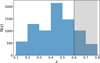Fig. 1. Distribution of the clusters as a function of redshift. Objects with z > 0.6, not considered in the cosmological analysis, are covered by the shaded grey area.

2.2. Mass proxy

We exploit the cluster shear signal through a stacked weak lensing analysis to estimate the mean cluster masses in bins of intrinsic richness and redshift. The intrinsic richness, λ^*, is defined as the following:

$$\begin{array}{c}\hfill {\lambda }_j^{\ast }={\displaystyle \sum _{i=1}^{N_{\mathrm{gal}}}}{P}_i(j)\text{with}\{\begin{array}{c}{m}_i<m^{\ast }(z_j)+1.5\hfill \\ R_i(j)<R_{\max }(z_j)\hfill \end{array},\end{array}$$(1)

where P_i(j) is the probability assigned by AMICO to the ith galaxy of being a member of a given detection j (see Maturi et al. 2019). The intrinsic richness thus represents the sum of the membership probabilities, that is the weighted number of visible galaxies belonging to a detection, under the conditions given by Eq. (1). The sum of the membership probabilities is an excellent estimator of the true number of member galaxies, as shown in Bellagamba et al. (2018) by running the AMICO algorithm on mock catalogues (see Fig. 8 in the reference). In particular, in Eq. (1), z_j is the redshift of the jth detected cluster, m_i is the magnitude of the ith galaxy, and R_i corresponds to the distance of the ith galaxy from the centre of the cluster. The parameter R_max(z_j) represents the radius enclosing a mass M₂₀₀ = 10¹⁴ M_⊙ h⁻¹, such that the corresponding mean density is 200 times the critical density of the Universe at the given redshift z_j. In the following analysis, indeed, we consider the masses evaluated as M₂₀₀. Lastly, m^* is the typical magnitude of the Schechter function in the cluster model assumed in the AMICO algorithm. We use the term intrinsic richness as opposed to apparent richness, defined in Maturi et al. (2019). In particular, since the threshold in absolute magnitude is always lower than the survey limit, thanks to its redshift dependence, λ^* does not depend on the survey limit. Conversely, the apparent richness is a quantity that includes all visible galaxies and is therefore related to how a cluster is observed given a certain apparent magnitude limit.

We set λ^* = 20 as the threshold for the counts’ analysis in order to exclude the bins affected by detection impurities and severe incompleteness. Thus the final sample of galaxy clusters considered for the counts’ analysis contains 3652 objects, with λ^* ≥ 20, and in the redshift bins z ∈ [0.1, 0.3], z ∈ [0.3, 0.45], and z ∈ [0.45, 0.6]. With regard to the binning in intrinsic richness, we adopt four logarithmically spaced bins in the range λ^* ∈ [20,  137] for each redshift bin. To test the robustness of our results with respect to this binning choice, we repeated the analysis assuming different numbers of λ^* bins and obtained negligible differences in the final results, that is to say far below the 1σ of the posterior distributions, and values of reduced χ² always consistent with 1. On the other hand, as we discuss in the next section, in order to fully exploit the available data, we did not impose any threshold in λ^* in the weak lensing masses analysis, and we chose a different binning in λ^*. To test the reliability of this approach, we also performed the cosmological analysis by imposing λ^* ≥ 20 for the weak lensing masses, deriving results fully in agreement with those obtained without assuming this threshold, as detailed in Sect. 4.

2.3. Weak lensing masses

To estimate the mean masses of the observed galaxy clusters, we followed the same stacked weak lensing procedure described in Bellagamba et al. (2019), based on KiDS-450 data. The clusters selected for the weak lensing analysis lie in the redshift range z ∈ [0.1, 0.6], over an effective area of 360.3 deg². This area is slightly smaller compared to that considered for the counts’ analysis since it was derived from the masking described in Hildebrandt et al. (2017). Despite the availability of galaxy clusters up to z = 0.8 in the AMICO KiDS-DR3 catalogue, the S/N of the stacked shear profiles is too low to perform the stacking for z > 0.6. Therefore we base our analysis on the redshift bins z ∈ [0.1, 0.3], z ∈ [0.3, 0.45], and z ∈ [0.45, 0.6], deriving the estimated mean masses in a flat ΛCDM cosmology with Ω_m = 0.3 and h = 0.7.

With an MCMC analysis, we sampled the posterior distributions of the base 10 logarithm of the estimated mean cluster masses, $log{\overline{M}}_{200}$, in 14 bins of intrinsic richness and redshift, considering λ^* ≥ 0 for a total of 6962 objects (see Table 1). As detailed in Sect. 3.4, we account for the systematic errors affecting the weak lensing mass estimates by relying on the results found in Bellagamba et al. (2019). Specifically, we consider the systematics due to background selection, photo-zs, and shear measurements, affecting the measured stacked cluster profiles. Such errors are then propagated into the mass estimates. In particular, the sum in quadrature of such contributions to systematic errors, along with those produced by the halo model, orientation, and projections, is equal to 7.6%. The description of the modelling, including a more extensive discussion on the statistical and systematic uncertainties, is detailed in Bellagamba et al. (2019).

The $log{\overline{M}}_{200}$ posteriors are marginalised over the other parameters entering the modelling, that is the concentration parameter, c₂₀₀, the fraction of haloes belonging to the miscentred population, f_off, and the root mean square deviation (rms) of the distribution of the halo misplacement on the plane of the sky, σ_off. In particular, we derived the posteriors for c₂₀₀, f_off, and σ_off in each bin, assuming the following flat priors: c₂₀₀ ∈ [1,  20], f_off ∈ [0,  0.5], and σ_off ∈ [0 Mpc h⁻¹,  0.5 Mpc h⁻¹]. Such parameters are not constrained by the data, that is their posteriors are statistically consistent with the priors. For what concerns the miscentring parameters, they are related to the possible difference between the centre defined by the AMICO algorithm using the galaxy overdensities and the mass centre related to the weak lensing signal. The uncertainty due to the use of a grid in AMICO indeed only impacts small scales not used in this analysis and thus they can be neglected.

The logarithm of the estimated mean mass values for different bins of intrinsic richness and redshift are listed in Table 1. In Fig. 2 we show the median value of the mass-intrinsic richness scaling relation, described in Sect. 3.1, obtained by only performing the modelling of the weak lensing masses as in Bellagamba et al. (2019), along with the 68% confidence level obtained from the analysis of cluster counts and weak lensing masses, detailed in Sect. 3. It turns out that the log M₂₀₀ − logλ^* relation is reasonably linear and with an intrinsic scatter of ∼0.1, as we discuss in Sect. 4, indicating the reliability of λ^* as a mass proxy.

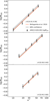Fig. 2. Logarithm of the masses in units of (1014 M⊙ h−1), $log{\overline{M}}_{200}$, from the AMICO KiDS-DR3 cluster catalogue as a function of the intrinsic richness λ*, in the redshift bins z ∈ [0.10,  0.30], z ∈ [0.30,  0.45], and z ∈ [0.45,  0.60], from top to bottom. The black triangles represent the mean values of $log{\overline{M}}_{200}$, given by the mean of the marginalised posterior obtained in the weak lensing analysis, while the error bars are given by 1σ of the posterior distribution. The orange lines represent the median scaling relation obtained by modelling only $log{\overline{M}}_{200}$, following the procedure described in Bellagamba et al. (2019). The grey bands represent the 68% confidence level derived from the multivariate posterior of all the free parameters considered in the cosmological analysis described in Sect. 3.

2.4. Selection function

In order to estimate the selection function of the AMICO KiDS-DR3 cluster catalogue, we make use of the mock catalogue described in Maturi et al. (2019). The construction of the mock clusters is based on the original galaxy dataset, thus all the properties of the survey are properly taken into account, such as masks, photo-z uncertainties, and the clustering of galaxies. In this way the assumptions necessary to build up the mock catalogue are minimised. In particular, regarding the photo-z uncertainties, the galaxies are drawn from the survey sample and selected from bins of richness and redshift, using a Monte Carlo sampling based on the cluster membership probability. The probability that each galaxy is included in a given redshift bin is driven by its own photo-z probability distribution function, which includes the contribution of the photometric noise. In this way, the selection of the simulated cluster member galaxies mimics the real uncertainties of the photometric redshifts in the photometric catalogue. Then, to derive the selection function, the AMICO code was run on the mock catalogue, consisting of 9018 clusters distributed over a total area of 189 deg². Only the detections with an S/N > 3.5 are considered, with this being the threshold applied to the real dataset.

In Fig. 3 we show the purity and completeness of the dataset, which define the selection function. The completeness is defined as the number of detections correctly identified as clusters over the total number of mock clusters as a function of redshift and intrinsic richness. Thus it provides a measure of how many objects are lost in the detection procedure. On the other hand, the purity is a measure of the contamination level of the cluster sample. It is defined as the fraction of detections matching the clusters in the mock catalogue, over the total number of detections, in a given bin of redshift and intrinsic richness. As shown in Fig. 3, it turns out that the catalogue is highly pure, with a purity approaching 100% over the whole redshift range for λ^* ≥ 20.

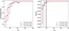Fig. 3. Completeness (left panel) and purity (right panel) of the AMICO KiDS-DR3 cluster catalogue as a function of the redshift, z, and of the intrinsic richness, λ*. The completeness is a function of the true λ*, i.e. ${\lambda }_{\text{tr}}^{*}$, while the purity is defined as a function of the observed intrinsic richness, ${\lambda }_{\text{ob}}^{*}$. The shaded area in the right panel highlights the bins excluded from the number counts’ analysis, i.e. for ${\lambda }_{\text{ob}}^{*}$ < 20.

In order to account for the selection function in the modelling of cluster counts, we built a new dataset by applying the purity and the completeness to the real cluster catalogue. This dataset will be used to derive the multiplicative weights that will be considered in the cluster counts’ model, as we detail in the following. Since we define the purity as a function of the observed intrinsic richness, ${\lambda }_{\text{ob}}^{*}$, we assigned each object in the real catalogue to a bin of observed intrinsic richness, in which we computed the purity. Subsequently, we extracted a uniform random number between 0 and 1, and if it is lower than the purity corresponding to the bin, the object is considered in the aforementioned new dataset. Otherwise, it is rejected. In this way, the final sample will statistically take the effects of impurities into account. On the other hand, since the completeness is defined in bins of true intrinsic richness, ${\lambda }_{\text{tr}}^{*}$, it is required to implement a method that assigns a value of completeness to an observed value of intrinsic richness. For this purpose, we derived several probability distributions from the mock catalogue describing the probability to obtain a true value of λ^*, given a range of observed intrinsic richness defined by ${\lambda }_{\mathrm{ob}}^{\ast \text{low}}$ and ${\lambda }_{\mathrm{ob}}^{\ast \text{up}}$, namely $P({\lambda }_{\mathrm{tr}}^{\ast }|{\lambda }_{\mathrm{ob}}^{\ast \text{low}},{\lambda }_{\mathrm{ob}}^{\ast \text{up}})$. We find that these distributions are reasonably Gaussian. Then, given a galaxy cluster in our dataset with a value of ${\lambda }_{\text{ob}}^{*}$ in a given range, we performed a Gaussian Monte Carlo extraction from $P({\lambda }_{\mathrm{tr}}^{\ast }|{\lambda }_{\mathrm{ob}}^{\ast \text{low}},{\lambda }_{\mathrm{ob}}^{\ast \text{up}})$ through which we obtain a value of ${\lambda }_{\text{tr}}^{*}$. Given the extracted true value of intrinsic richness, we assigned a completeness value to the considered object. Having this new catalogue corrected for the purity and the completeness, we constructed a weight factor defined as the ratio between the uncorrected counts and the corrected ones for bins in intrinsic richness (denoted by $\mathrm{\Delta }{\lambda }_{\text{ob},i}^{*}$) and redshift (labelled as Δz_ob, j). These weight factors, w($\mathrm{\Delta }{\lambda }_{\text{ob},i}^{*}$, Δz_ob, j), will be used to weigh the counts’ model as described in Sect. 3.2. The value of w($\mathrm{\Delta }{\lambda }_{\text{ob},i}^{*}$, Δz_ob, j) in the first bins of intrinsic richness amounts to ∼0.87, ∼0.76, and ∼0.64 in the redshift bins z ∈ [0.10,  0.30], z ∈ [0.30,  0.45], and z ∈ [0.45,  0.60], respectively, while we derived no correction for the other bins (i.e. in these bins the weights are equal to 1). The measured counts of the AMICO KiDS-DR3 clusters are shown in Fig. 4, along with the 68% confidence level derived in Sect. 4.

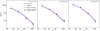Fig. 4. Number counts from the AMICO KiDS-DR3 cluster catalogue as a function of the intrinsic richness λ*, in the redshift bins z ∈ [0.10,  0.30], z ∈ [0.30,  0.45], and z ∈ [0.45,  0.60], from left to right. The black dots represent the counts directly retrieved from the catalogue, where the error bars are given by the Poissonian noise. The solid blue lines represent the model computed by assuming the cosmological parameters obtained by Planck Collaboration VI (2020) (Table 2, TT, TE, and EE+lowE), while the red dashed lines show the results based on the WMAP cosmological parameters (Hinshaw et al. 2013) (Table 3, WMAP-only Nine-year). Both in the Planck and WMAP cases, the scaling relation parameters and the intrinsic scatter have been fixed to the median values listed in Table 2, retrieved from the modelling. The grey bands represent the 68% confidence level derived from the multivariate posterior of all the free parameters considered in the cosmological analysis.

3. Modelling

3.1. Model for the weak lensing masses

We modelled the scaling relation between the estimated cluster mean masses and the intrinsic richnesses using the following functional form:

$$\begin{array}{cc}\hfill log\frac{M_{200}}{{10}^{14}{M}_{\odot }/h}& =\alpha +\beta {\displaystyle {\int }_0^{\infty }\mathrm{d}{\lambda }^{\ast }P({\lambda }^{\ast }|{\lambda }_{\mathrm{eff}}^{\ast })log\frac{{\lambda }^{\ast }}{{\lambda }_{\mathrm{piv}}^{\ast }}}\hfill \\ \hfill & +\gamma {\displaystyle {\int }_0^{\infty }\mathrm{d}zP(z|z_{\mathrm{eff}})log\frac{E(z)}{E(z_{\mathrm{piv}})},}\hfill \end{array}$$(2)

where E(z)≡H(z)/H₀, while z_eff and ${\lambda }_{\text{eff}}^{*}$ are the lensing-weighted effective redshift and richness, respectively, whose computation is described in Bellagamba et al. (2019). The probability distributions P(λ^*|${\lambda }_{\text{eff}}^{*}$) and P(z|z_eff) are assumed to be Gaussian, with a mean equal to the values of ${\lambda }_{\text{eff}}^{*}$ and z_eff listed in Table 1, and an rms given by the uncertainties on ${\lambda }_{\text{eff}}^{*}$ and z_eff, respectively. The last term in Eq. (2) accounts for deviations in the redshift evolution from what is predicted in the self-similar growth scenario (Sereno & Ettori 2015). Following Bellagamba et al. (2019), we set ${\lambda }_{\text{piv}}^{*}=30$ and z_piv = 0.35. In Eq. (2) the observables are the estimated mean mass values, $log{\overline{M}}_{200}$, shown in Table 1, along with the effective values of redshift, z_eff, and of intrinsic richness, λ_eff, in the given bin. Furthermore, since $log{\overline{M}}_{200}$ depends on cosmological parameters, we adopted the rescaling described in Sereno (2015), that is

$$\begin{array}{c}\hfill {\overline{M}}_{200,\mathrm{new}}={\overline{M}}_{200,\mathrm{ref}}\frac{{\left[D_d^{-\frac{3\delta \gamma }{2-\delta \gamma }}{\left(\frac{D_{\mathrm{ds}}}{D_{\mathrm{s}}}\right)}^{-\frac{3}{2-\delta \gamma }}H{(z)}^{-\frac{1+\delta \gamma }{1-\delta \gamma /2}}\right]}_{\mathrm{new}}}{{\left[D_d^{-\frac{3\delta \gamma }{2-\delta \gamma }}{\left(\frac{D_{\mathrm{ds}}}{D_{\mathrm{s}}}\right)}^{-\frac{3}{2-\delta \gamma }}H{(z)}^{-\frac{1+\delta \gamma }{1-\delta \gamma /2}}\right]}_{\mathrm{ref}}},\end{array}$$(3)

where ref indicates the assumed reference cosmology, in other words Ω_m = 0.3 and h = 0.7, while the subscript new refers to that of the test. We set the slope to δγ = 0, corresponding to the case of a singular isothermal profile, with this being a good approximation in general (as discussed in Sereno 2015). For example, assuming M₂₀₀ ≃ 10¹⁵  M_⊙ and c₂₀₀ ≃ 3, δγ ≃ −0.1 is obtained, thus we varied δγ in the reasonable range [ − 0.2, 0.2] and verified that this does not have an impact on the final results. The terms D_s, D_d, and D_ds are the source’s, the lens’, and the lens-source’s angular diameter distances, respectively. In D_d, D_ds, and in the Hubble parameter, H(z), we assumed the effective redshift values, z_eff, listed in Table 1. With regard to the redshifts of the sources, we considered the lensed source effective redshifts, z_s,eff, listed in Table 1, obtained by following the procedure described in Giocoli et al. (2021). In particular, we obtained z_s,eff by weighting the redshift of each source by the corresponding source density for each derived radial bin for each cluster. We then considered the mean value of source redshift in bins of cluster richness per redshift. We verified that we can neglect the uncertainty on z_s,eff in our analysis. In such mass rescaling, the relative uncertainty on $log{\overline{M}}_{200,\mathrm{new}}$ is constant, corresponding to the relative errors on $log{\overline{M}}_{200,\mathrm{ref}}$.

3.2. Model for the cluster counts

The specific characteristics of the dataset must be included in the model and in the covariance matrix of the likelihood function. We describe the expectation value of the counts in a given bin of intrinsic richness, $\mathrm{\Delta }{\lambda }_{\text{ob},i}^{\ast }$, and of observed redshift, Δz_ob, j, as

$$\begin{array}{cc}\hfill ⟨N(\mathrm{\Delta }{\lambda }_{\text{ob},i}^{\ast },\mathrm{\Delta }{z}_{\text{ob},j})⟩& =w(\mathrm{\Delta }{\lambda }_{\text{ob},i}^{\ast },\mathrm{\Delta }{z}_{\text{ob},j})\mathrm{\Omega }{\displaystyle \underset{0}{\overset{\infty }{\int }}\mathrm{d}{z}_{\mathrm{tr}}\frac{\mathrm{d}V}{\mathrm{d}{z}_{\mathrm{tr}}\mathrm{d}\mathrm{\Omega }}}\hfill \\ \hfill & \times {\displaystyle \underset{0}{\overset{\infty }{\int }}\mathrm{d}{M}_{\mathrm{tr}}\frac{\mathrm{d}n(M_{\mathrm{tr}},z_{\mathrm{tr}})}{\mathrm{d}{M}_{\mathrm{tr}}}\underset{0}{\overset{\infty }{\int }}\mathrm{d}{\lambda }_{\mathrm{tr}}^{\ast }P({\lambda }_{\mathrm{tr}}^{\ast }|M_{\mathrm{tr}},z_{\mathrm{tr}})}\hfill \\ \hfill & \times {\displaystyle \underset{\mathrm{\Delta }{z}_{\text{ob},j}}{\int }\mathrm{d}{z}_{\mathrm{ob}}P(z_{\mathrm{ob}}|z_{\mathrm{tr},\mathrm{corr}})\underset{\mathrm{\Delta }{\lambda }_{\text{ob},i}^{\ast }}{\int }\mathrm{d}{\lambda }_{\mathrm{ob}}^{\ast }P({\lambda }_{\mathrm{ob}}^{\ast }|{\lambda }_{\mathrm{tr}}^{\ast }),}\hfill \end{array}$$(4)

where z_tr is the true redshift, V is the co-moving volume, Ω is the survey effective area, M_tr is the true mass, and dn(M_tr, z_tr)/dM_tr is the mass function, for which the model by Tinker et al. (2008) is assumed. The term w($\mathrm{\Delta }{\lambda }_{\text{ob},i}^{*}$, Δz_ob, j) is the weight factor described in Sect. 2.4, accounting for the purity and completeness of the sample. The probability distribution P(z_ob|z_{tr,  corr}), assessed through the mock catalogue described in Sect. 2.4, is a Gaussian accounting for the uncertainties on the redshifts. The mean of such distribution, z_{tr,  corr}, is the true redshift corrected by the redshift bias, and it is expressed as

$$\begin{array}{c}\hfill z_{\mathrm{tr},\mathrm{corr}}=z_{\mathrm{tr}}+\mathrm{\Delta }{z}_{\mathrm{bias}}(1+z_{\mathrm{tr}}),\end{array}$$(5)

where Δz_bias (1 + z_tr) is the redshift bias term discussed in Maturi et al. (2019), with Δz_bias = 0.02. In particular, this bias corresponds to what was found in de Jong et al. (2017) by comparing the KiDS photo-zs to the GAMA spectroscopic redshifts (see their Table 8). In order to assess the impact of its uncertainty, we included Δz_bias as a free parameter in the model, assuming a Gaussian prior with a mean equal to 0.02 and an rms equal to 0.02, which is similar to the rms of the sample and much larger than the rms of the mean (see Fig. 7 in Maturi et al. 2019). As we verified, such uncertainty on Δz_bias does not significantly impact our final results. Conversely, AMICO provides unbiased estimates of redshift (see Maturi et al. 2019), thus we modelled P(z_ob|z_tr) by keeping the mean of such distributions fixed to the central value of Δz_tr. In particular, in the mock catalogue, we measured P(z_ob|z_tr) in several bins of z_tr, namely Δz_tr, and we performed the statistical MCMC analysis assuming a common flat prior on the rms in all the Δz_tr bins. The resulting rms of P(z_ob|z_tr) is equal to 0.025. AMICO also provides unbiased estimates for λ^*, thus following the same procedure adopted for P(z_ob|z_tr), we derived an uncertainty of ∼17% on ${\lambda }_{\text{ob}}^{*}$, defining the rms of the Gaussian distribution P(${\lambda }_{\text{ob}}^{*}$|${\lambda }_{\text{tr}}^{*}$), whose mean is equal to ${\lambda }_{\text{tr}}^{*}$. We neglected the uncertainties on the rms of P(z_ob|z_tr) and P(${\lambda }_{\text{ob}}^{*}$|${\lambda }_{\text{tr}}^{*}$), amounting to ∼1%, since we verified their negligible effect on the final results.

Furthermore, P(${\lambda }_{\text{tr}}^{*}$|M_tr, z_tr) is a probability distribution that weights the expected counts according to the shape of the mass-observable scaling relation, and it is expressed as follows:

$$\begin{array}{c}\hfill P({\lambda }_{\mathrm{tr}}^{\ast }|M_{\mathrm{tr}},z_{\mathrm{tr}})=\frac{P(M_{\mathrm{tr}}|{\lambda }_{\mathrm{tr}}^{\ast },z_{\mathrm{tr}})P({\lambda }_{\mathrm{tr}}^{\ast }|z_{\mathrm{tr}})}{P(M_{\mathrm{tr}}|z_{\mathrm{tr}})},\end{array}$$(6)

where the distribution P(M_tr|${\lambda }_{\text{tr}}^{*}$, z_tr) is a log-normal one whose mean is given by the mass-observable scaling relation and the standard deviation is given by the intrinsic scatter, σ_intr, set as a free parameter of the model:

$$\begin{array}{c}\hfill P(log{M}_{\mathrm{tr}}|{\lambda }_{\mathrm{tr}}^{\ast },z_{\mathrm{tr}})=\frac{1}{\sqrt{2\pi }{\sigma }_{\mathrm{intr}}}exp(-\frac{x^2(M_{\mathrm{tr}},{\lambda }_{\mathrm{tr}}^{\ast },z_{\mathrm{tr}})}{2{\sigma }_{\mathrm{intr}}^2}),\end{array}$$(7)

where

$$\begin{array}{cc}\hfill x(M_{\mathrm{tr}},{\lambda }_{\mathrm{tr}}^{\ast },z_{\mathrm{tr}})=& log\frac{M_{\mathrm{tr}}}{{10}^{14}{M}_{\odot }/h}\hfill \\ \hfill & -(\alpha +\beta log\frac{{\lambda }_{\mathrm{tr}}^{\ast }}{{\lambda }_{\mathrm{piv}}^{\ast }}+\gamma log\frac{E(z_{\mathrm{tr}})}{E(z_{\mathrm{piv}})})\hfill \end{array}$$(8)

and

$$\begin{array}{c}\hfill {\sigma }_{\mathrm{intr}}={\sigma }_{\mathrm{intr},0}+{\sigma }_{\mathrm{intr},{\lambda }^{\ast }}log\frac{{\lambda }_{\mathrm{tr}}^{\ast }}{{\lambda }_{\mathrm{piv}}^{\ast }}.\end{array}$$(9)

The P(M_tr|${\lambda }_{\text{tr}}^{*}$, z_tr) distribution indeed accounts for the intrinsic uncertainty that affects a scaling relation between the intrinsic richness and the mass: given an infinitely accurate scaling relation, represented by the mean, the cluster mass provided by a value of intrinsic richness is scattered from the true value. Furthermore, P(${\lambda }_{\text{tr}}^{*}$|Δz_tr) in Eq. (6) is a power law with an exponential cut-off, derived from the mock catalogue by considering the objects with ${\lambda }_{\text{tr}}^{*}$ ≳ 20. Specifically, similar to other literature analyses (e.g. Murata et al. 2019; Costanzi et al. 2019; Abbott et al. 2020), P(${\lambda }_{\text{tr}}^{*}$|M_tr, z_tr) is assumed to be cosmology-independent. Thus we assume that the ratio ${\lambda }_{\text{tr}}^{*}$|z_tr)/P(M_tr|z_tr) is cosmology-independent, where P(M_tr|z_tr) acts as a normalisation of P(${\lambda }_{\text{tr}}^{*}$|M_tr, z_tr):

$$\begin{array}{c}\hfill P(M_{\mathrm{tr}}|z_{\mathrm{tr}})={\displaystyle \underset{0}{\overset{\infty }{\int }}\mathrm{d}{\lambda }_{\mathrm{tr}}^{\ast }P(M_{\mathrm{tr}}|{\lambda }_{\mathrm{tr}}^{\ast },z_{\mathrm{tr}})P({\lambda }_{\mathrm{tr}}^{\ast }|z_{\mathrm{tr}}).}\end{array}$$(10)

3.3. Halo mass function systematics

As mentioned in Sect. 3.2, we assume the Tinker et al. (2008) halo mass function to model the observed cluster counts. Following Costanzi et al. (2019), in order to characterise the systematic uncertainty in the halo mass function in dark matter only simulations, we related the Tinker et al. (2008) mass function to the true mass function via

$$\begin{array}{c}\hfill n(M,z)=n{(M,z)}^{\mathrm{Tinker}}(slog(M/M^{\ast })+q),\end{array}$$(11)

where log M^* = 13.8 h⁻¹ M_⊙ is the pivot mass, while q and s are free parameters of the model with a Gaussian prior having the following covariance matrix:

$$\begin{array}{c}\hfill C(\overline{s},\overline{q})=\left(\begin{array}{cc}0.00019& 0.00024\\ 0.00024& 0.00038\end{array}\right),\end{array}$$(12)

and with $\overline{s}=0.037$ and $\overline{q}=1.008$ as the mean values. Diagonalising the matrix (12), we obtained the following 1D Gaussian priors: $\mathcal{N}(\overline{s},{\sigma }_{\mathrm{s}})=\mathcal{N}(0.037,0.014)$, and $\mathcal{N}(\overline{q},{\sigma }_{\mathrm{q}})=\mathcal{N}(1.008,0.019)$, where 𝒩(μ, σ) stands for a Gaussian distribution with mean μ and standard deviation σ.

3.4. Likelihood

Our likelihood function encapsulates the description of cluster counts and weak lensing masses. We base the likelihood term describing the counts, ℒ_counts, on the functional form given by Lacasa & Grain (2019), that is to say a convolution of a Poissonian likelihood describing the counts, and a Gaussian distribution accounting for the super-sample covariance (SSC):

$$\begin{array}{cc}\hfill {\mathcal{L}}_{\mathrm{counts}}=& {\displaystyle \int }\mathrm{d}{\mathit{\delta }}_{\mathrm{b}}^{n_{\mathrm{z}}}{\displaystyle \left[\prod _{i,j}\text{Poiss}(N_{i,j}|{\overline{N}}_{i,j}+\frac{\partial N_{i,j}}{\partial {\delta }_{\text{b},j}}{\delta }_{\text{b},j})\right]\mathcal{N}({\mathit{\delta }}_{\mathrm{b}}|0,S).}\hfill \end{array}$$(13)

In the equation above, 𝒩(δ_b|0, S) is the Gaussian function describing the SSC effects on cluster count measurements, which is a function of the matter density contrast fluctuation, δ_b, and has a covariance matrix S¹⁰. In particular, n_z is the number of redshift bins considered in the modelling procedure, and it defines the dimension of the integration variable, δ_b = {δ_b, 1, …, δ_b, nz}, and of the S matrix, whose dimension is n_z × n_z. Thus each δ_b, j represents the fluctuation of the measured matter density contrast, with respect to the expected one, in a given bin of redshift. The indices i and j are the labels of the bins of intrinsic richness and redshift, while N_i, j ≡ N($\mathrm{\Delta }{\lambda }_{\text{ob},i}^{*}$, Δz_ob, j) is the observed cluster number counts in a bin of intrinsic richness and redshift, and ${\overline{N}}_{i,j}$ is the model defined in Eq. (4). The term ∂N_i, j/∂δ_b, j is the response of the counts, that is the measure of how the counts vary with changes of the background density, and it is expressed as follows:

$$\begin{array}{cc}\hfill \frac{\partial N_{i,j}}{\partial {\delta }_{\text{b},j}}& =w(\mathrm{\Delta }{\lambda }_{\text{ob},i}^{\ast },\mathrm{\Delta }{z}_{\text{ob},j})\mathrm{\Omega }{\displaystyle \underset{0}{\overset{\infty }{\int }}\mathrm{d}{z}_{\mathrm{tr}}\frac{\mathrm{d}V}{\mathrm{d}{z}_{\mathrm{tr}}\mathrm{d}\mathrm{\Omega }}}\hfill \\ \hfill & \times {\displaystyle \underset{0}{\overset{\infty }{\int }}\mathrm{d}{M}_{\mathrm{tr}}\frac{\mathrm{d}n(M_{\mathrm{tr}},z_{\mathrm{tr}})}{\mathrm{d}{M}_{\mathrm{tr}}}b(M_{\mathrm{tr}},z_{\mathrm{tr}})\underset{0}{\overset{\infty }{\int }}\mathrm{d}{\lambda }_{\mathrm{tr}}^{\ast }P({\lambda }_{\mathrm{tr}}^{\ast }|M_{\mathrm{tr}},z_{\mathrm{tr}})}\hfill \\ \hfill & \times {\displaystyle \underset{\mathrm{\Delta }{z}_{\text{ob},j}}{\int }\mathrm{d}{z}_{\mathrm{ob}}P(z_{\mathrm{ob}}|z_{\mathrm{tr},\mathrm{corr}})\underset{\mathrm{\Delta }{\lambda }_{\text{ob},i}^{\ast }}{\int }\mathrm{d}{\lambda }_{\mathrm{ob}}^{\ast }P({\lambda }_{\mathrm{ob}}^{\ast }|{\lambda }_{\mathrm{tr}}^{\ast }),}\hfill \end{array}$$(14)

in other words, the response is similar to the model described in Eq. (4), in which we also include the contribution of the linear bias b(M, z).

For computational purposes, we consider in the analysis an alternative form of the likelihood, ${\mathcal{L}}_{\text{counts}}^{\prime }$, that is the integrand in Eq. (13), of which we computed the natural logarithm:

$$\begin{array}{c}\hfill ln{\mathcal{L}}_{\mathrm{counts}}^{\prime }=ln{\displaystyle [\prod _{i,j}\text{Poiss}(N_{i,j}|{\overline{N}}_{i,j}+\frac{\partial N_{i,j}}{\partial {\delta }_{\text{b},j}}{\delta }_{\text{b},j})·\mathcal{N}({\mathit{\delta }}_{\text{b}}|0,S)].}\end{array}$$(15)

Here, we set δ_b = {δ_b, 1, …, δ_b, nz} as free parameters of the model, with a multivariate Gaussian prior having S as the covariance matrix. Due to the dependence on cosmological parameters of the S matrix, the values of its elements change at every step of the MCMC. In turn, a variation of S implies the change of the prior on δ_b. At the end of the MCMC, we marginalised over δ_b to derive the posteriors of our parameters of interest.

With regard to the likelihood describing the weak lensing masses, ℒ_lens, we assumed a log-normal functional form and then we considered its natural logarithm:

$$\begin{array}{c}\hfill ln{\mathcal{L}}_{\mathrm{lens}}\propto {\displaystyle \sum _{k=1}^{N_{\mathrm{bin}}}\sum _{l=1}^{N_{\mathrm{bin}}}[log{\overline{M}}_{\mathrm{ob}}^k-log{\overline{M}}_{\mathrm{mod}}^l]{\mathit{C}}_{M,kl}^{-1}[log{\overline{M}}_{\mathrm{ob}}^l-log{\overline{M}}_{\mathrm{mod}}^k],}\end{array}$$(16)

where N_bin corresponds to the number of bins in which the mean mass ${\overline{M}}_{200}$, or ${\overline{M}}_{\mathrm{ob}}$, was measured, through the weak lensing analysis described in Sect. 2.3. Furthermore, ${\overline{M}}_{\mathrm{mod}}$ represents the mass obtained from the scaling relation model described in Eq. (2), where we assumed the effective redshift and intrinsic richness values z_eff and ${\lambda }_{\text{eff}}^{*}$ listed in Table 1. The covariance matrix C_M in Eq. (16) has the following form:

$$\begin{array}{c}\hfill {\mathit{C}}_{M,kl}={\delta }_{\mathit{kl}}{E}_k^2+{[{\sigma }_{\mathrm{sys}}/ln(10)]}^2+{\delta }_{\mathit{kl}}{({\sigma }_{\mathrm{intr}}/\sqrt{N_{\mathrm{cl}}})}^2,\end{array}$$(17)

where E_k represents the statistical error on $log{\overline{M}}_{\mathrm{ob}}$ derived from the posterior distribution of $log{\overline{M}}_{\mathrm{ob}}$, where we stress that the relative uncertainties are constants after the rescaling described in Sect. 2.3. The term σ_sys = 0.076 is the sum in quadrature of the uncertainties on the background selection, photo-zs, shear measurements, halo model, orientation, and projections, obtained in Bellagamba et al. (2019), and N_cl is the number of clusters in the bin of intrinsic richness and redshift in which the mean mass has been derived. By dividing σ_intr by $\sqrt{N_{\mathrm{cl}}}$, we neglected the cluster clustering contribution to the last term of Eq. (17).

Thus, the logarithm of the joint likelihood, lnℒ, is given by

$$\begin{array}{c}\hfill ln\mathcal{L}=ln{\mathcal{L}}_{\mathrm{counts}}^{\prime }+ln{\mathcal{L}}_{\mathrm{lens}}.\end{array}$$(18)

4. Results

We performed a cosmological analysis of cluster number counts and stacked weak lensing based on the assumption of a flat ΛCDM model. The aim is to constrain the matter density parameter, Ω_m, and the square root of the mass variance computed on a scale of 8 Mpc h⁻¹ and σ₈, with both being provided at z = 0, along with the parameters defining the scaling relation between masses and intrinsic richnesses, α, β, and γ in Eq. (2), and the intrinsic scatter, σ_intr. Therefore we set Ω_m, σ₈, α, β, γ, and σ_intr as free parameters of the model, Eq. (4), as well as the baryon density, Ω_b, the optical depth at re-ionisation, τ, the primordial spectral index, n_s, the normalised Hubble constant, h, the Tinker mass function correction parameters, q and s, described in Sect. 3.3, and the fluctuation of the mean density of matter due to super-survey modes, δ_b. We assumed flat priors for Ω_m, σ₈, α, β, γ, and σ_intr, while we set Gaussian priors on the other parameters (see Table 2). In particular, for the Gaussian prior distributions of Ω_b, τ, n_s, and h, we refer readers to the values obtained by the Planck Collaboration VI (2020) (Table 2, TT, TE, and EE+lowE+lensing), assuming the same mean values and imposing a standard deviation equal to 5σ for all the aforementioned parameters, but h, for which we assumed a standard deviation equal to 0.1. In this baseline cosmological model, we also assumed three neutrino species, approximated as two massless states and a single massive neutrino of mass m_ν = 0.06 eV, following Planck Collaboration VI (2020). Finally, we assumed a multivariate Gaussian prior for δ_b, as described in Sect. 3.4.

In our analysis, we constrained the value of the cluster normalisation parameter, S₈ ≡ σ₈(Ω_m/0.3)^0.5. The significance of this parameter is rooted in the degeneracy between σ₈ and Ω_m, being defined along the σ₈ − Ω_m confidence regions. Since the number of massive clusters increases with both σ₈ and Ω_m, in order to hold the cluster abundance fixed at its observed value, any increase in σ₈ must be compensated for by a decrease in Ω_m, implying that S₈ is held fixed.

From this modelling, we obtain ${\mathrm{\Omega }}_{\text{m}}={0.24}_{-0.04}^{+0.03}$, ${\sigma }_8={0.86}_{-0.07}^{+0.07}$, and $S_8={0.78}_{-0.04}^{+0.04}$, where we quote the median, 16th and 84th percentiles, as shown in Fig. 5 and Table 2. In Fig. 5 we also show that the results on the mass-observable scaling relation retrieved from this analysis, that is for α, β, and γ, are in agreement within 1σ with those obtained by performing the modelling of the weak lensing data only, as carried out by Bellagamba et al. (2019). In particular, the inclusion of the cluster counts in the analysis provides tighter constraints on the slope β, also governing the slope of the cluster model at low values of λ^*. Additionally, the cluster count redshift evolution provides a more accurate estimate of γ. Lastly, we find a tight constraint on the intrinsic scatter, deriving ${\sigma }_{\mathrm{intr},0}={0.18}_{-0.10}^{+0.08}$ and ${\sigma }_{\mathrm{intr},{\lambda }^{\ast }}={0.11}_{-0.22}^{+0.19}$, which confirms the reliability of λ^* as a mass proxy. This result on σ_intr is consistent within 1σ with that derived in Sereno et al. (2020) from a weak lensing analysis of the sample of AMICO clusters in KiDS-DR3.

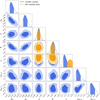Fig. 5. Constraints on Ωm, σ8, α, β, γ, σintr, 0, and σintr, λ*, derived in a flat ΛCDM universe by combining the redshift bins z ∈ [0.1,  0.3], z ∈ [0.3,  0.45], and z ∈ [0.45,  0.6] and assuming a minimum intrinsic richness ${\lambda }_{\text{ob}, \text{min}}^{*}=20$ for cluster counts. The shown posteriors were also marginalised over Ωb, τ, ns, h, s, q, and δb. The blue contours represent the results obtained from the joint analysis of cluster counts and weak lensing masses, while the orange contours show the posteriors on α, β, and γ, derived from the analysis including only the weak lensing masses as in Bellagamba et al. (2019). The confidence ellipses correspond to 68% and 95%, while the bands over the 1D marginalised posteriors represent the 68% of confidence.

As shown in Fig. 6, the constraints obtained for S₈ and σ₈ are in agreement within 1σ with WMAP results (Hinshaw et al. 2013) (Table 3, WMAP-only Nine-year), and with Planck results (Planck Collaboration VI 2020) (Table 2, TT, TE, and EE+lowE). With regard to Ω_m, we find an agreement within 1σ with WMAP and a 2σ tension with Planck. Furthermore, in Fig. 7 we show the comparison with the S₈ constraints obtained from additional external datasets. In particular, we find an agreement within 1σ with the results obtained from the cluster counts’ analyses performed by Costanzi et al. (2019), based on SDSS-DR8 data, and by Bocquet et al. (2019), based on the 2500 deg² SPT-SZ survey data, as well as with the results derived from the cosmic shear analyses performed by Troxel et al. (2018) on DES-Y1 data, Hikage et al. (2019) on HSC-Y1 data, and Asgari et al. (2021) on KiDS-DR4 data. The constraint on S₈ obtained from the cluster counts and weak lensing joint analysis in DES (Abbott et al. 2020), $S_8=0.{65}_{-0.04}^{+0.04}$, not shown in Fig. 7, is not consistent with our result.

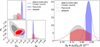Fig. 6. Comparison with WMAP and Planck results. Left panel: we show the Ωm − σ8 parameter space, along with the 1D marginalised posteriors with the relative intervals between the 16th and 84th percentiles, in the case of the cluster counts’ analysis in the AMICO KiDS-DR3 catalogue (solid grey lines). In the same panel, we also display the results from WMAP (Hinshaw et al. 2013) (Table 3, WMAP-only Nine-year; red dash-dotted lines) and Planck (Planck Collaboration VI 2020) (Table 2, TT, TE, and EE+lowE; blue dashed lines). Right panel: we show the posteriors for the parameter S8, where the bands show the intervals between 16th and 84th percentiles. The symbols are the same as in the left panel.

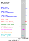Fig. 7. Comparison of the constraints on S8 ≡ σ8(Ωm/0.3)0.5 obtained, from top to bottom, from the joint analysis of cluster counts and weak lensing in the AMICO KiDS-DR3 catalogue (black dot), from the results obtained by Planck Collaboration VI (2020) (blue dots), Hinshaw et al. (2013) (red dots), Costanzi et al. (2019) (green dot), Bocquet et al. (2019) (brown dot), Troxel et al. (2018) (magenta dot), Hikage et al. (2019) (orange dot), and Asgari et al. (2021) (cyan dot). The median, as well as the 16th and 84th percentiles are shown.

Following a more conservative approach, we repeated the analysis also assuming the threshold in intrinsic richness λ^* ≥ 20 for the weak lensing data. This leads to ${\mathrm{\Omega }}_{\mathrm{m}}=0.{27}_{-0.05}^{+0.04}$, ${\sigma }_8=0.{83}_{-0.07}^{+0.06}$, and $S_8=0.{78}_{-0.04}^{+0.04}$, which are consistent within 1σ with the constraints derived from the analysis previously described. Also for the other free parameters of the model, the consistency within 1σ still holds.

5. Conclusions

We performed a galaxy cluster abundance analysis in the AMICO KiDS-DR3 catalogue (Maturi et al. 2019), simultaneously constraining the cosmological parameters and the cluster mass-observable scaling relation. In particular, we relied on the intrinsic richness, defined in Eq. (1), as the observable linked to the cluster masses. The sample exploited for cluster counts includes 3652 galaxy clusters having an intrinsic richness of λ^* ≥ 20 and, in the redshift bins, z ∈ [0.1, 0.3], z ∈ [0.3, 0.45], and z ∈ [0.45, 0.6]. For the weak lensing analysis, we followed the procedure developed by Bellagamba et al. (2019), not assuming any threshold in λ^*. We assessed the incompleteness and the impurities of the cluster sample by exploiting a mock catalogue developed by Maturi et al. (2019), and we corrected our data accordingly.

We assumed a model for cluster counts, shown in Eq. (4), accounting for the redshift uncertainties and for the mass-observable scaling relation. In particular, the mass-observable scaling relation plays a crucial role in the P(${\lambda }_{\text{tr}}^{*}$|M_tr, z_tr) term given by Eq. (6), which also depends on the observed distribution of galaxy clusters as a function of the intrinsic richness. Furthermore, this term includes the contribution of the intrinsic scatter of the scaling relation, σ_intr, which is considered as an unknown parameter. Subsequently, we modelled the cluster counts and the scaling relation by combining the relative likelihood functions.

Assuming a flat ΛCDM model with massive neutrinos, we found ${\mathrm{\Omega }}_{\text{m}}={0.24}_{-0.04}^{+0.03}$, ${\sigma }_8={0.86}_{-0.07}^{+0.07}$, and $S_8={0.78}_{-0.04}^{+0.04}$, which are competitive constraints, in terms of uncertainties, with results from state-of-the-art cluster number counts’ analyses. In addition, the result on S₈ is in agreement within 1σ with the results from WMAP and Planck. We also derived results for the scaling relation that are consistent within 1σ with those obtained by only modelling the weak lensing signal as in Bellagamba et al. (2019), thus validating the reliability of our model. With regard to the intrinsic scatter, we found ${\sigma }_{\mathrm{intr},0}={0.18}_{-0.10}^{+0.08}$ and ${\sigma }_{\mathrm{intr},{\lambda }^{\ast }}={0.11}_{-0.22}^{+0.19}$, which is a very competitive result compared to the present-day estimates in the field of galaxy clusters, outlining the goodness of the assumption of λ^* as the mass proxy.

In Nanni (in prep.), we analyse the AMICO KiDS-DR3 cluster clustering to derive constraints on S₈ and on the mass-observable scaling relation. For the next step, we combine counts, clustering, and weak lensing to improve the accuracy of our results further. In addition, we expect more accurate constraints on S₈ and on the mass-observable scaling relation from the analysis of the latest KiDS Data Release (DR4, Kuijken et al. 2019). It covers an area of 1000 square degrees, which is more than two-thirds of the final area, and photometry extends to the near-infrared (ugriZYJHK_s), joining the data from the KiDS and VIKING (Edge et al. 2013) surveys, thus allowing, for instance, one to improve the photometric redshift estimates (Wright et al. 2019).

Acknowledgments

Based on data products from observations made with ESO Telescopes at the La Silla Paranal Observatory under programme IDs 177.A-3016, 177.A3017 and 177.A-3018, and on data products produced by Target/OmegaCEN, INAF-OACN, INAF-OAPD and the KiDS production team, on behalf of the KiDS consortium. The authors acknowledge the use of computational resources from the parallel computing cluster of the Open Physics Hub (https://site.unibo.it/openphysicshub/en) at the Physics and Astronomy Department in Bologna. FM, LM and CG acknowledge the support from the grant ASI n.2018-23-HH.0. LM and CG also acknowledge the support from the grant PRIN-MIUR 2017 WSCC32. MS acknowledges financial contribution from contract ASI-INAF n.2017-14-H.0 and INAF mainstream project 1.05.01.86.10. We thank Andrea Biviano, Matteo Costanzi, Catherine Heymans and Konrad Kuijken for their valuable advice. We also thank Fabien Lacasa for the support in the development of an optimal numerical implementation of the likelihood function describing the cluster counts, that is Eq. (15).

References

All Tables

All Figures

	Fig. 1. Distribution of the clusters as a function of redshift. Objects with z > 0.6, not considered in the cosmological analysis, are covered by the shaded grey area.
In the text

Fig. 2. Logarithm of the masses in units of (1014 M⊙ h−1), $log{\overline{M}}_{200}$, from the AMICO KiDS-DR3 cluster catalogue as a function of the intrinsic richness λ*, in the redshift bins z ∈ [0.10,  0.30], z ∈ [0.30,  0.45], and z ∈ [0.45,  0.60], from top to bottom. The black triangles represent the mean values of $log{\overline{M}}_{200}$, given by the mean of the marginalised posterior obtained in the weak lensing analysis, while the error bars are given by 1σ of the posterior distribution. The orange lines represent the median scaling relation obtained by modelling only $log{\overline{M}}_{200}$, following the procedure described in Bellagamba et al. (2019). The grey bands represent the 68% confidence level derived from the multivariate posterior of all the free parameters considered in the cosmological analysis described in Sect. 3.

In the text

Fig. 3. Completeness (left panel) and purity (right panel) of the AMICO KiDS-DR3 cluster catalogue as a function of the redshift, z, and of the intrinsic richness, λ*. The completeness is a function of the true λ*, i.e. ${\lambda }_{\text{tr}}^{*}$, while the purity is defined as a function of the observed intrinsic richness, ${\lambda }_{\text{ob}}^{*}$. The shaded area in the right panel highlights the bins excluded from the number counts’ analysis, i.e. for ${\lambda }_{\text{ob}}^{*}$ < 20.

In the text

Fig. 4. Number counts from the AMICO KiDS-DR3 cluster catalogue as a function of the intrinsic richness λ*, in the redshift bins z ∈ [0.10,  0.30], z ∈ [0.30,  0.45], and z ∈ [0.45,  0.60], from left to right. The black dots represent the counts directly retrieved from the catalogue, where the error bars are given by the Poissonian noise. The solid blue lines represent the model computed by assuming the cosmological parameters obtained by Planck Collaboration VI (2020) (Table 2, TT, TE, and EE+lowE), while the red dashed lines show the results based on the WMAP cosmological parameters (Hinshaw et al. 2013) (Table 3, WMAP-only Nine-year). Both in the Planck and WMAP cases, the scaling relation parameters and the intrinsic scatter have been fixed to the median values listed in Table 2, retrieved from the modelling. The grey bands represent the 68% confidence level derived from the multivariate posterior of all the free parameters considered in the cosmological analysis.

In the text

Fig. 5. Constraints on Ωm, σ8, α, β, γ, σintr, 0, and σintr, λ*, derived in a flat ΛCDM universe by combining the redshift bins z ∈ [0.1,  0.3], z ∈ [0.3,  0.45], and z ∈ [0.45,  0.6] and assuming a minimum intrinsic richness ${\lambda }_{\text{ob}, \text{min}}^{*}=20$ for cluster counts. The shown posteriors were also marginalised over Ωb, τ, ns, h, s, q, and δb. The blue contours represent the results obtained from the joint analysis of cluster counts and weak lensing masses, while the orange contours show the posteriors on α, β, and γ, derived from the analysis including only the weak lensing masses as in Bellagamba et al. (2019). The confidence ellipses correspond to 68% and 95%, while the bands over the 1D marginalised posteriors represent the 68% of confidence.

In the text

Fig. 6. Comparison with WMAP and Planck results. Left panel: we show the Ωm − σ8 parameter space, along with the 1D marginalised posteriors with the relative intervals between the 16th and 84th percentiles, in the case of the cluster counts’ analysis in the AMICO KiDS-DR3 catalogue (solid grey lines). In the same panel, we also display the results from WMAP (Hinshaw et al. 2013) (Table 3, WMAP-only Nine-year; red dash-dotted lines) and Planck (Planck Collaboration VI 2020) (Table 2, TT, TE, and EE+lowE; blue dashed lines). Right panel: we show the posteriors for the parameter S8, where the bands show the intervals between 16th and 84th percentiles. The symbols are the same as in the left panel.

In the text

Fig. 7. Comparison of the constraints on S8 ≡ σ8(Ωm/0.3)0.5 obtained, from top to bottom, from the joint analysis of cluster counts and weak lensing in the AMICO KiDS-DR3 catalogue (black dot), from the results obtained by Planck Collaboration VI (2020) (blue dots), Hinshaw et al. (2013) (red dots), Costanzi et al. (2019) (green dot), Bocquet et al. (2019) (brown dot), Troxel et al. (2018) (magenta dot), Hikage et al. (2019) (orange dot), and Asgari et al. (2021) (cyan dot). The median, as well as the 16th and 84th percentiles are shown.

In the text

References

- Abbott, T. M. C., Aguena, M., Alarcon, A., et al. 2020, Phys. Rev. D, 102, 023509 [Google Scholar]
- Allen, S. W., Evrard, A. E., & Mantz, A. B. 2011, ARA&A, 49, 409 [Google Scholar]
- Amendola, L., Appleby, S., Avgoustidis, A., et al. 2018, Liv. Rev. Rel., 21, 2 [Google Scholar]
- Angulo, R. E., Springel, V., White, S. D. M., et al. 2012, MNRAS, 426, 2046 [NASA ADS] [CrossRef] [Google Scholar]
- Asgari, M., Lin, C.-A., Joachimi, B., et al. 2021, A&A, 645, A104 [NASA ADS] [CrossRef] [EDP Sciences] [Google Scholar]
- Balmès, I., Rasera, Y., Corasaniti, P. S., & Alimi, J. M. 2014, MNRAS, 437, 2328 [CrossRef] [Google Scholar]
- Bardeau, S., Soucail, G., Kneib, J. P., et al. 2007, A&A, 470, 449 [NASA ADS] [CrossRef] [EDP Sciences] [Google Scholar]
- Bellagamba, F., Roncarelli, M., Maturi, M., & Moscardini, L. 2018, MNRAS, 473, 5221 [NASA ADS] [CrossRef] [Google Scholar]
- Bellagamba, F., Sereno, M., Roncarelli, M., et al. 2019, MNRAS, 484, 1598 [Google Scholar]
- Bocquet, S., Saro, A., Dolag, K., & Mohr, J. J. 2016, MNRAS, 456, 2361 [Google Scholar]
- Bocquet, S., Dietrich, J. P., Schrabback, T., et al. 2019, ApJ, 878, 55 [Google Scholar]
- Böhringer, H., Schuecker, P., Guzzo, L., et al. 2004, A&A, 425, 367 [NASA ADS] [CrossRef] [EDP Sciences] [Google Scholar]
- Borgani, S., & Kravtsov, A. 2011, Adv. Sci. Lett., 4, 204 [Google Scholar]
- Castro, T., Borgani, S., Dolag, K., et al. 2021, MNRAS, 500, 2316 [Google Scholar]
- Clerc, N., Adami, C., Lieu, M., et al. 2014, MNRAS, 444, 2723 [NASA ADS] [CrossRef] [Google Scholar]
- Corasaniti, P.-S., Sereno, M., & Ettori, S. 2021, ApJ, 911, 82 [NASA ADS] [CrossRef] [Google Scholar]
- Costanzi, M., Rozo, E., Simet, M., et al. 2019, MNRAS, 488, 4779 [NASA ADS] [CrossRef] [Google Scholar]
- Cui, W., Borgani, S., Dolag, K., Murante, G., & Tornatore, L. 2012, MNRAS, 423, 2279 [NASA ADS] [CrossRef] [Google Scholar]
- Dark Energy Survey Collaboration (Abbott, T., et al.) 2016, MNRAS, 460, 1270 [Google Scholar]
- de Jong, J. T. A., Verdoes Kleijn, G. A., Boxhoorn, D. R., et al. 2015, A&A, 582, A62 [NASA ADS] [CrossRef] [EDP Sciences] [Google Scholar]
- de Jong, J. T. A., Verdoes Kleijn, G. A., Erben, T., et al. 2017, A&A, 604, A134 [NASA ADS] [CrossRef] [EDP Sciences] [Google Scholar]
- Despali, G., Giocoli, C., Angulo, R. E., et al. 2016, MNRAS, 456, 2486 [NASA ADS] [CrossRef] [Google Scholar]
- Edge, A., Sutherland, W., Kuijken, K., et al. 2013, The Messenger, 154, 32 [NASA ADS] [Google Scholar]
- Euclid Collaboration (Adam, R., et al.) 2019, A&A, 627, A23 [NASA ADS] [CrossRef] [EDP Sciences] [Google Scholar]
- Giocoli, C., Tormen, G., & Sheth, R. K. 2012, MNRAS, 422, 185 [NASA ADS] [CrossRef] [Google Scholar]
- Giocoli, C., Moscardini, L., Baldi, M., Meneghetti, M., & Metcalf, R. B. 2018, MNRAS, 478, 5436 [Google Scholar]
- Giocoli, C., Marulli, F., Moscardini, L., et al. 2021, A&A, 653, A19 [NASA ADS] [CrossRef] [EDP Sciences] [Google Scholar]
- Hikage, C., Oguri, M., Hamana, T., et al. 2019, PASJ, 71, 43 [Google Scholar]
- Hildebrandt, H., Viola, M., Heymans, C., et al. 2017, MNRAS, 465, 1454 [Google Scholar]
- Hilton, M., Hasselfield, M., Sifón, C., et al. 2018, ApJS, 235, 20 [Google Scholar]
- Hinshaw, G., Larson, D., Komatsu, E., et al. 2013, ApJS, 208, 19 [Google Scholar]
- Hoekstra, H., Mahdavi, A., Babul, A., & Bildfell, C. 2012, MNRAS, 427, 1298 [NASA ADS] [CrossRef] [Google Scholar]
- Kuijken, K. 2011, The Messenger, 146, 8 [NASA ADS] [Google Scholar]
- Kuijken, K., Heymans, C., Dvornik, A., et al. 2019, A&A, 625, A2 [NASA ADS] [CrossRef] [EDP Sciences] [Google Scholar]
- Lacasa, F., & Grain, J. 2019, A&A, 624, A61 [NASA ADS] [CrossRef] [EDP Sciences] [Google Scholar]
- Laureijs, R., Amiaux, J., Arduini, S., et al. 2011, ArXiv e-prints [arXiv:1110.3193] [Google Scholar]
- LSST Dark Energy Science Collaboration 2012, ArXiv e-prints [arXiv:1211.0310] [Google Scholar]
- Martinet, N., Schneider, P., Hildebrandt, H., et al. 2018, MNRAS, 474, 712 [Google Scholar]
- Marulli, F., Veropalumbo, A., & Moresco, M. 2016, Astron. Comput., 14, 35 [Google Scholar]
- Marulli, F., Veropalumbo, A., Moscardini, L., Cimatti, A., & Dolag, K. 2017, A&A, 599, A106 [NASA ADS] [CrossRef] [EDP Sciences] [Google Scholar]
- Marulli, F., Veropalumbo, A., Sereno, M., et al. 2018, A&A, 620, A1 [NASA ADS] [CrossRef] [EDP Sciences] [Google Scholar]
- Marulli, F., Veropalumbo, A., García-Farieta, J. E., et al. 2021, ApJ, 920, 13 [Google Scholar]
- Maturi, M., Meneghetti, M., Bartelmann, M., Dolag, K., & Moscardini, L. 2005, A&A, 442, 851 [NASA ADS] [CrossRef] [EDP Sciences] [Google Scholar]
- Maturi, M., Fedeli, C., & Moscardini, L. 2011, MNRAS, 416, 2527 [Google Scholar]
- Maturi, M., Bellagamba, F., Radovich, M., et al. 2019, MNRAS, 485, 498 [Google Scholar]
- Melchior, P., Suchyta, E., Huff, E., et al. 2015, MNRAS, 449, 2219 [NASA ADS] [CrossRef] [Google Scholar]
- Miyazaki, S., Oguri, M., Hamana, T., et al. 2018, PASJ, 70, S27 [NASA ADS] [Google Scholar]
- Murata, R., Oguri, M., Nishimichi, T., et al. 2019, PASJ, 71, 107 [CrossRef] [Google Scholar]
- Okabe, N., Zhang, Y. Y., Finoguenov, A., et al. 2010, ApJ, 721, 875 [NASA ADS] [CrossRef] [Google Scholar]
- Pacaud, F., Pierre, M., Melin, J. B., et al. 2018, A&A, 620, A10 [NASA ADS] [CrossRef] [EDP Sciences] [Google Scholar]
- Pierre, M., Pacaud, F., Adami, C., et al. 2016, A&A, 592, A1 [NASA ADS] [CrossRef] [EDP Sciences] [Google Scholar]
- Planck Collaboration VI. 2020, A&A, 641, A6 [NASA ADS] [CrossRef] [EDP Sciences] [Google Scholar]
- Reischke, R., Maturi, M., & Bartelmann, M. 2016, MNRAS, 456, 641 [NASA ADS] [CrossRef] [Google Scholar]
- Rykoff, E. S., Rozo, E., Busha, M. T., et al. 2014, ApJ, 785, 104 [Google Scholar]
- Sartoris, B., Biviano, A., Fedeli, C., et al. 2016, MNRAS, 459, 1764 [Google Scholar]
- Schrabback, T., Applegate, D., Dietrich, J. P., et al. 2018, MNRAS, 474, 2635 [Google Scholar]
- Sereno, M. 2015, MNRAS, 450, 3665 [Google Scholar]
- Sereno, M., & Ettori, S. 2015, Nat. Comm., 6, 7211 [NASA ADS] [CrossRef] [Google Scholar]
- Sereno, M., Veropalumbo, A., Marulli, F., et al. 2015, MNRAS, 449, 4147 [NASA ADS] [CrossRef] [Google Scholar]
- Sereno, M., Ettori, S., Lesci, G. F., et al. 2020, MNRAS, 497, 894 [NASA ADS] [CrossRef] [Google Scholar]
- Shan, H., Liu, X., Hildebrandt, H., et al. 2018, MNRAS, 474, 1116 [Google Scholar]
- Sheth, R. K., & Tormen, G. 1999, MNRAS, 308, 119 [Google Scholar]
- Stern, C., Dietrich, J. P., Bocquet, S., et al. 2019, MNRAS, 485, 69 [NASA ADS] [CrossRef] [Google Scholar]
- Tinker, J., Kravtsov, A. V., Klypin, A., et al. 2008, ApJ, 688, 709 [Google Scholar]
- Troxel, M. A., MacCrann, N., Zuntz, J., et al. 2018, Phys. Rev. D, 98 [Google Scholar]
- Velliscig, M., van Daalen, M. P., Schaye, J., et al. 2014, MNRAS, 442, 2641 [Google Scholar]
- Veropalumbo, A., Marulli, F., Moscardini, L., Moresco, M., & Cimatti, A. 2014, MNRAS, 442, 3275 [NASA ADS] [CrossRef] [Google Scholar]
- Veropalumbo, A., Marulli, F., Moscardini, L., Moresco, M., & Cimatti, A. 2016, MNRAS, 458, 1909 [NASA ADS] [CrossRef] [Google Scholar]
- Vikhlinin, A., Kravtsov, A. V., Burenin, R. A., et al. 2009, ApJ, 692, 1060 [Google Scholar]
- Watson, W. A., Iliev, I. T., D’Aloisio, A., et al. 2013, MNRAS, 433, 1230 [Google Scholar]
- Wright, A. H., Hildebrandt, H., Kuijken, K., et al. 2019, A&A, 632, A34 [NASA ADS] [CrossRef] [EDP Sciences] [Google Scholar]
All Tables
Parameters considered in the joint analysis of cluster counts and stacked weak lensing data.