| Issue |
A&A
Volume 658, February 2022
|
|
|---|---|---|
| Article Number | A201 | |
| Number of page(s) | 8 | |
| Section | Planets and planetary systems | |
| DOI | https://doi.org/10.1051/0004-6361/202142874 | |
| Published online | 24 February 2022 | |
Understanding the interior structure of gaseous giant exoplanets with machine learning techniques
1
State Key Laboratory of Lunar and Planetary Sciences, Macau University of Science and Technology,
Macau,
PR China
e-mail: This email address is being protected from spambots. You need JavaScript enabled to view it.
2
CNSA Macau Center for Space Exploration and Science,
Macau,
PR China
3
Key Laboratory of Tropical Atmosphere-Ocean System, Ministry of Education,
Zhuhai,
PR China
Received:
10
December
2021
Accepted:
20
January
2022
Abstract
Context. Characterizing the interiors of gaseous giant exoplanets is currently one of the main objectives in exoplanetary sciences. In particular, the planetary heavy-element mass provides a critical constraint on planet formation from exoplanetary systems. However, gas giant exoplanets show large diversities in thermal states and their interior properties vary across a wide magnitude range. Forward modeling of their interiors exhibits a larger degeneracy with respect to rocky exoplanets.
Aims. We applied machine learning techniques based on mixture density networks (MDNs) to investigate the interiors of gaseous giant exoplanets. We aim to provide a well-trained MDN for quick and efficient predictions.
Methods. Based on our current knowledge of gas giants in the Solar System, we discussed an effect of model uncertainties on planetary interiors and presented a data set for gas giants with masses between 0.1 and 10 Jupiter masses using two-layer interior models. Then, MDNs were constructed to train the generated data set and their performance was evaluated in order to achieve a well-trained one.
Results. The MDN using planetary mass and radius as inputs exhibits the well-known degeneracy of interior models. The surface temperature of a planet bears constraints on the thermal state of planetary interiors, and adding it as additional input considerably breaks the degeneracy of possible interior structures. The MDN with inputs of mass, radius, and surface temperature is found to show excellent performance in predicting the interior properties of gaseous giant exoplanets, although these interior properties span over a very wide range. We also applied the well-trained MDN to four gas giants in the Solar System and beyond. The MDN predictions are in good agreement with the interior model solutions within the observational and systematic uncertainties.
Conclusions. We offer a convenient and powerful tool available online providing knowledge of the interiors of gaseous giant exoplanets in addition to rocky exoplanets, which could be helpful for our understanding of planet formation in diverse protoplanetary environments.
Key words: methods: numerical / planets and satellites: gaseous planets / planets and satellites: interiors
© ESO 2022
1 Introduction
The past detection and characterization of exoplanets have provided rich information on their macroscopic properties such as orbital parameters, bulk properties (mass, radius, equilibrium temperature), and properties of their host stars. We are now moving from the discovery phase to a new era where we attempt to understand the atmospheric process and internal structure of exoplanets. Modeling the interior of exoplanets is currently one of the hot topics in exoplanetary sciences, yielding more findings than measurements of planetary mass and radius. Exoplanets are extremely diverse in the Universe, including terrestrial and oceanic Earth-sized planets, super-Earths, icy Neptune-like planets, and gas giants (Batalha 2014; Spiegel et al. 2014). The interior characterization of Earth-sized exoplanets mostly resorts to terrestrial bulk compositions from the knowledge of terrestrial planets in our Solar System (Sotin et al. 2007; Boujibar et al. 2020; Zhao & Ni 2021). Bulk refractory abundances from observations of host star’s photospheric compositions can be used to constrain the interior models of super-Earths and sub-Neptunes (Valencia et al. 2007; Dorn et al. 2017; Brugger et al. 2017; Adibekyan et al. 2021). For gas giants where direct measurements of their atmospheres are possible for transiting exoplanets, atmospheric observations show large diversities in effective temperature and most of these gas giants have no direct analogues in our Solar System in terms of physical and orbital parameters. Despite this, the internal structure and interior composition of gas giants have been explored within a similar model for Solar System giants (Nettelmann et al. 2010; Kramm et al. 2012). Thermal and structural evolution models have also been constructed to constrain the interior structures of gas giant exoplanets (Guillot & Showman 2002; Guillot 2005; Fortney et al. 2011; Thorngren et al. 2016; Fortney et al. 2021), which play a crucial role in understanding planet formation in diverse protoplanetary environments. Various interior models with different focuses have been developed for interior characterization. These models are capable of interpreting the measured mass and radius within their uncertainties. But they exhibit an inherent degeneracy issue as two planetary bodies with different internal structures or compositions could have the same mass and radius. In order to address the degeneracy issue, some inversion methods and new observations are proposed to constrain the interior structure of exoplanets. Rogers & Seager (2010) and Dorn et al. (2015, 2017) performed a full probabilistic inverse analysis of planetary compositions for rocky exoplanets with the uncertainties of measurements and models. Nettelmann et al. (2010) and Kramm et al. (2012) showed that the tidal Love number k2 is a useful observable constraint on the interior models of gas giants, reducing the inherent degeneracy of interior models.
More recently, a wide range of machine learning techniques have been applied to Earth and planetary sciences, such as random forests (RFs), deep neural networks (DNNs), and mixture density networks (MDNs). The RF and DNN algorithms have powerful abilities in extracting information from high-dimensional data. In regression tasks, the objective of RFs and DNNs is to use some input variables to predict one or more variables, yielding discrete values for output variables. They have been widely applied to various fields in recent years, including exoplanet characterization (Ulmer-Moll et al. 2019), planetary growth models (Alibert & Venturini 2019), and the volcanic origin on Earth (Zhao et al. 2019). However, both RFs and DNNs show mediocre performance on degenerate problems where one set of input variables yields more than one solution for one output variable (Bishop 1994). The MDN algorithm is thus developed for degenerate cases without sacrificing degenerate solutions. It combines the structure of a conventional neural network with a probability mixture model, yielding multimodal probability distributions for output variables. MDNs have been shown by Atkins et al. (2016) to be a powerful method to infer the governing parameters for mantle convection. MDNs have also been shown by Baumeister et al. (2020) to be a useful tool to infer the distribution of possible thicknesses of each planetary layer for exoplanets with 0.01 M⊕ < M < 25 M⊕. Very recently, we trained MDNs to predict the radial structure and core properties of rocky exoplanets with 0.1 M⊕ < M < 10 M⊕ (Zhao & Ni 2021).This motivates further investigations of how the MDN works for understanding the interior of gaseous giant exoplanets. Gas giant exoplanets span over a much wider range of physical conditions than rocky exoplanets. In particular, they show larger diversities in thermal states. For example, their core properties and amounts of heavy elements are varied by several orders of magnitude and they are divided into cool, warm, and hot Jupiters according to thermal conditions. This brings about some difficulties for the trained MDN to accurately predict the interior properties of gas giant exoplanets. Nevertheless, once a MDN modelis well trained, users can quickly assess the interior structure of planets without calculating any additional interior models. In Sect. 2, we describe the interior model of gaseous giant exoplanets and present the practical aspects of internal structure calculations. Then we briefly introduce the MDN algorithm applied in this field in Sect. 3 since more details on MDNs have already been explained in the works of Baumeister et al. (2020) and Zhao & Ni (2021). Section 4 presents our results of the MDN training and testing, followed by the applications of the trained MDN to four representative gas giants. The predictive ability of the trained MDN is discussed in detail. Finally, the main results of this paper are summarized in Sect. 5.
2 Interior structure models and training data sets
The standard structure equations for a rotating body are as follows:
 (1)
(1)
 (2)
(2)
 (3)
(3)
where ρ is the density at mean radius r, m is the mass enclosed within meanradius r, ω is the planet’s angular velocity, and∇T is the temperaturegradient ∇T ≡ (d lnT∕d lnP) which is equal to ∇ad in the adiabatic case. The closure of the above system of Eqs. (1)–(3) requires the equation of state (EOS) of the H–He–rock–ice mixture, namely the density as a function of temperature, pressure, and composition. For hydrogen and helium, we chose to use the recent Chabrier et al. (2019) EOSs for pure hydrogen and helium, namely CMS19. The calculations of Chabrier et al. (2019) combined ab initio simulations for intermediate-density matter with semi-analytical calculations for low-density and high-density matter, spanning over a wide range of densities from 10−8 to 106 g cm−3, with pressures from 10−9 to 1013 GPa and temperatures from 102 to 108 K. The heavy elements, which can be divided into ices and rocks, are assumed to be either water for ices or serpentine for rocks (Thorngren et al. 2016). Here we adopt a 50–50 ice–rock mixture and use the Thompson (1990) ANEOS EOS for heavy elements. The EOS of the H–He–rock–ice mixture is generated using the separate EOSs for pure species in terms of the additive volume rule. The density for the mixture is therefore approximated at any given pressure P, temperature T, and composition (X, Y, and Z) as
 (4)
(4)
where the rock mass fraction in heavy elements frock is fixed at 0.50 as stated above.
For gas giants in our Solar System, the current knowledge from both observational and theoretical sides have demonstrated some inhomogeneities in their interiors, such as the hydrogen–helium immiscibility region in Saturn (Leconte & Chabrier 2013; Schöttler & Redmer 2018; Mankovich & Fortney 2020; Brygoo et al. 2021) and the dilute core region in Jupiter (Wahl et al. 2017; Guillot et al. 2018; Ni 2019). For a planet with an inhomogeneous layer inside, the inhomogeneous layer would reduce the outward heat transport, causing the deeper interior to get hotter and exhibit lower densities. Such a density deficit would be compensated by adding more heavy elements in the interior in order to comply with the measured mass and radius of the planet (Ni 2019; Nettelmann et al. 2021). Atmosphere grids, which serve as an upper boundary condition for interior models, have been computed through radiative–convective equilibrium atmosphere models to constrain the atmospheric structure and thermal evolution of gas giants (Fortney et al. 2007, 2011). Fortney et al. (2007) computed grids of radiative-convective model atmospheres for hydrogen–helium planets on a large grid of gravities, intrinsic effective temperatures, and incident fluxes. For a highly irradiated hot Jupiter or an old and relatively low-mass planet where incident stellar flux dominates over intrinsic flux, an atmospheric radiative region grows and quickly becomes almost isothermal (Guillot & Showman 2002; Fortney et al. 2007). The appearance of isothermal regions makes the deep interior adiabat cooler than the adiabatic case. This is indeed the opposite in regards to the appearance of inhomogeneous regions.
Atmosphere grids for Jupiter and Saturn were also computed by Fortney et al. (2011) over a range of intrinsic fluxes and surface gravities. These grids provide the temperature at the 10-bar level T10 over a wide range of the intrinsic effective temperature Tint and surface gravity g. However, they could not cover all atmospheric conditions of giant planets along the evolutionary track. In order to cover more atmospheric conditions, Leconte & Chabrier (2013) made an extrapolation by an analytic fit T10 (Tint, g) to the numerical grids of Fortney et al. (2011). Here, we adopted Jupiter’s analytic function T10 (Tint, g) to infer the intrinsic temperature Tint of the modeled planet with a given temperature T10 and gravity g. This procedure works well for Jupiter-like giants. For strongly irradiated planets such as hot Jupiters, Guillot & Showman (2002) showed the atmosphere grids suitable for isolated objects would overestimate the atmospheric temperature. In turn, the isolated case only provides a lower boundto Tint. Various atmospheric processes affecting the atmospheric temperature are very complex and beyond the scope of this work.
The uncertainties from internal structures and atmospheric grids are often overshadowed by large uncertainties in available observationsof mass, radius, and effective temperature for gas giant exoplanets. In this work, we do not attempt to consider all the modeling uncertainties, but grasp the key ingredients to make the generated data as realistic as possible. We modeled the internal structure of gaseous giant exoplanets using two-layer structure models. A gaseous exoplanet consists of an isothermal central compact core made of heavy elements and a homogenous convective envelope composed of hydrogen–helium mixtures with a certain amount of heavy elements. Following the interior models of gas giants in our Solar System, we define the surface of gaseous giant exoplanets as the 1-bar pressure level and set the temperature at the 1-bar level as T1. The mass fractions of helium and heavy elements in the envelope are denoted by Y and Z, respectively. The Y∕(1 − Z) value was constrained so that the mean helium mass fraction of the planet would match the value in the protosolar nebula Yproto∕(Xproto + Yproto) = 0.277 ± 0.006 (Serenelli & Basu 2010; Guillot et al. 2018). The central compact core, which is full of heavy elements, has the mass of Mcore and its thermal state is characterized by the pressure and temperature at the core-envelope boundary (CEB), PCEB and TCEB. Figure 1 illustrates a schematic diagram of the interior structure of gaseous giant exoplanets.
Giant planets in our Solar System serve as calibrators for the interior modeling of gas giant exoplanets. In generating the training data sets, we imposed the following constraints on our interior models based on our current knowledge of gas giants, especially the ones in our Solar System. We first focused our attention to gas giant exoplanets with masses M between 0.1 and 10 Jupiter masses (MJ), and the core mass Mcore was randomly sampled between 0 and 50 M⊕. Owing to planet rotations, a first-order correction to the gravitational potential appears in the hydrostatic equilibrium Eq. (1). Here, the rotation period of modeled exoplanets, hardly having an influence on planetary interiors, was set to a random value between 0.1 and 10.0 days. Many gas giant exoplanets are much closer to their host stars and hence much hotter than gas giants in our Solar System. So the surface temperature T1 was randomly sampled between 100 to 3000 K. As for the heavy-element abundance Z in the envelope, it is known that Jupiter’s atmosphere exhibits the heavy-element enrichment that is about 3 times that of solar abundances and Saturn’s atmosphere is more enriched in heavy elements by a factor of roughly 10 relative to solar abundances. With this in mind, the heavy-element abundance Z is assumed to randomly vary between 1.0 and 20.0 times solar abundances. We note that these restrictions do not cover all gaseous giant exoplanets. After initializing the interior structure of modeled planets, we numerically integrated the system of Eqs. (1)–(3) until convergence. In total, we obtained ~200 000 data points for the training data set.
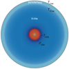 |
Fig. 1 Schematic interior structure of gaseous giant exoplanets. The compact core with mass Mcore is characterized by the pressure and temperature at the core envelope boundary (CEB), PCEB and TCEB. The surface defined by the 1-bar pressure level is characterized by the temperature T1 bar and the deeper atmosphere at the 10-bar pressure level by the temperature T10 bar. |
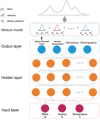 |
Fig. 2 Sketch map of the mixture density network (MDN) where Gaussian mixture models are combined with the neural network. Three hidden layers are involved in the neutral network and each layer has 512 neurons. Twenty Gaussian mixture components are involved in the mixture model and each component is characterized by means μ, variances σ2, and mixing coefficients α. |
3 Machine learning approaches
3.1 Mixture density networks
In most recent years, MDN technology, composed of neural networks and mixture models, has been successfully applied to characterize the interior structure of exoplanets (Baumeister et al. 2020; Zhao & Ni 2021), where the multimodal probability distribution instead of one discrete value is predicted for each output variable. Figure 2 illustrates the MDN structure with Gaussian mixture models combined with the neural network. Following Zhao & Ni (2021), three hidden layers with 512 neurons each were used. That is, a neural network of “Input–512–512–512–Output” was built. For the output layer, a linear association of 20 Gaussian mixture components was adopted for each output variable and each Gaussian mixture component was characterized by means μ, variances σ2, and mixing coefficients α.
The data we generated using the above interior models are randomly divided into training and testing data sets by a ratio of nine to one. And 10% of the training data set was used as a validation data set to validate the model results at the end of each epoch. The Adaptive moment estimation (Adam) optimizer (Kingma & Ba 2014)with a learning rate of 0.001 was chosen in the training process and Rectified Linear Unit (ReLU) functions were used to activate the hidden layers. The mixture model layer uses logit functions for mixing coefficients α neurons and nonnegative exponential linear unit (NNELU) functions for μ and σ2 neurons. Early-stopping (Montavon et al. 2012) and dropout (Srivastava et al. 2014) methods were employed in the MDN training to avoid the occurrence of overfitting. Min-max normalization was used in order to prevent introducing any bias in the model training. The difference between the MDN outputs and the target data was measured by the so-called loss function and the average negative log-likelihood (NLL) was adopted,
![Mathematical equation: \begin{equation*}\mathcal{L}(\Theta)\,{=}\,{-}\frac{1}{N}\sum_{(\mathbf{x},\mathbf{y})\in\mathbb{D}}\log\Bigg{[}\sum_{i=1}^{m}\alpha_{i}({\bm x})~\phi_{i}\Big{(}{\bm y}~|~\mu_{i}({\bm x}),\sigma_{i}^{2}({\bm x})\Big{)}\Bigg{]},\end{equation*}](/articles/aa/full_html/2022/02/aa42874-21/aa42874-21-eq5.png) (5)
(5)
where Θ represents the MDN model parameters, N is the size of the training data set  consisting of input vectors x and target vectors y, m is the number of the Gaussian mixture components, αi is the mixture weight of the ith Gaussian distribution, ϕi represents the ith Gaussian distribution of the target vector y, and μi and
  are the mean and variance of the ith Gaussian distribution. The iterative training process was performed by adjusting the weight values of the MDN until the NLL loss had a good convergence. Finally, the performance of the trained MDN model was assessed using the testing data set. More details about the MDN model can be found in Baumeister et al. (2020) and Zhao & Ni (2021).
Our MDN model was trained on NVIDIA GeForce GT 730 graphics card using Keras (Chollet et al. 2015) based on TensorFlow (Abadi et al. 2016) and MDN layers (Martin & Duhaime 2019). The scikit-learn library (Pedregosa et al. 2011) was used for data processing.
3.2 Model training and validation
Knowledge of the heavy-element mass of gas giants can provide important clues as to the mechanism of planet formation (Fortney et al. 2007; Thorngren et al. 2016). The heavy-element enrichment of Jupiter and Saturn, including their atmospheric compositions and core masses, have been extensively explored (Wahl et al. 2017; Guillot et al. 2018; Ni 2019; Militzer et al. 2019; Debras & Chabrier 2019; Mankovich & Fortney 2020; Ni 2020; Nettelmann et al. 2021), improving our understanding of planet formation. However, there is little knowledge of the bulk or atmosphericcompositions of exoplanets, providing much fewer constraints on planet formation from exoplanetary systems. In the MDN model, we pay particular attention to the heavy-element mass of gas giant exoplanets,  .
.
At present, direct measurements of an exoplanet’s atmosphere are possible for transiting gaseous exoplanets. One key diagnostic for a giant planet atmosphere is the equilibrium temperature Teq, which represents the energy flux received from its host star. It is dependent on the luminosity of the star, the planet’s Bond albedo, and the distance between the planet and star. Meanwhile, the total effective temperature Teff of a planet can be most easily derived from its experimentally measured infrared emission spectrum. The most unconstrained thermal quantity of a planet is the intrinsic effective temperature Tint, which varieswith the age and mass of a planet. We can express the total luminosity of a planet with radius R as
 (6)
(6)
After remote measurements of the total emitted infrared flux and the reflected visible flux, the radius R could be constrained from the known Tint according to Eq. (6) (Marley et al. 2007). The intrinsic temperature Tint is also among the most important quantities in planetary evolution calculations (Guillot & Showman 2002; Fortney et al. 2007, 2011; Thorngren et al. 2016). So, the intrinsic temperature Tint is predicted as one MDN output as well. As for the thermodynamics properties of planetary cores, the pressure and temperature at the CEB, PCEB and TCEB, are predicted from the MDN similar to the case of rocky exoplanets (Zhao & Ni 2021).
We designed two comparative MDN models, with (M, R) inputs and with (M, R, T1) inputs. First, we investigated how much data is required to train a good model by evaluating the performance of MDN fitting to the training data set of a different size. When the training data set reaches the size of 104, as shown in Fig. 3a, the NLL loss changes little over the size for both MDN models. For the sake of comprehensiveness, we used all the training data to train our MDN models. Figure 3b and c illustrates the learning curves of the two MDNs, where the training and validation losses are shown as a function of the training epoch. The validation NLL loss reaches an approximate constant after 80 epochs for both MDN models. This implies that continuing training could not further improve the performance of the MDN model. Additionally, the MDN with (M, R, T1) inputs yields the smaller NLL loss than the MDN with (M, R) inputs, suggesting its better training performance. After both MDN models were trained, the testing data set was fed to them to evaluate their performance in predicting the interior properties of gas giant exoplanets.
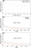 |
Fig. 3 Negative log-likelihood (NLL) loss for the MDN model trained on mass and radius inputs only and for the MDN model trained on mass, radius, and T1 inputs. (a) Dependence of the NLL loss on the size of the training data set for the two MDN models. (b) Learning curve of the MDN trained on mass and radius inputs only for both the training and validation data sets. (c) Learning curve of the MDN trained on mass, radius, and T1 inputs for both the training and validation data sets. |
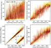 |
Fig. 4 Predicted distributions of four output variables from the MDN trained on (M, R) inputs versus the actual values obtained from the interior models for the testing data set: total heavy-element mass MZ, intrinsic effective temperature Tint, as well as pressure and temperature at the core envelope boundary (CEB), PCEB and TCEB. Blue dasheddiagonal lines denote a perfect performance of the MDN. The predicted distributions are colored according to the local probability density (the color scale is black at the maximum). |
4 Results
Figure 4 illustrates the ability of the MDN trained on mass and radius inputs only to predict the interior properties of gaseous giant exoplanets, where the distributions predicted by the MDN from the testing dataset are displayed versus the actual values obtained from the interior models. With only mass M and radius R as inputs, the MDN can infer the CEB pressure PCEB well. The similar behavior also emerged in the MDN predictions for rocky exoplanets (Zhao & Ni 2021). It is accounted for by a trade-off between the integral interval and pressure gradient of the hydrostatic Eq. (1). In contrast to the case of rocky exoplanets, the present MDN tends to overestimate the PCEB values for Jupiter-sized planets and underestimate the PCEB values for super-Jupiters. This can be easily understood because the present PCEB values span over a much wider range from 10−2 to 104 Mbar, leading to some difficulties for the MDN to accurately predict the whole set of PCEB. It is also becauseplanetary rotation affects the pressure profile of gas giants (see Eq. (1)), but the rotation period of a planet is not included as input to the MDN. It should be noted that these deviations from the actual PCEB values can be systematically ignored with respect to the large uncertainties in available observations of planetary mass and radius. The CEB temperature TCEB and intrinsic effective temperatureTint are moderately constrained since the adiabatic temperature gradient is primarily a function of the hydrostatic pressure (see Eq. (3)). For the total mass of heavy elements, the MDN predictions exhibit a broad distribution, showing the considerabledegeneracy of possible interior structures.
The surface temperature T1 is closely related to the thermal state of gas giants. It has been demonstrated by Baumeister et al. (2020) and Zhao & Ni (2021) that adding an additional input into the MDN could significantly improve the performance of the trained MDN. Therefore, the MDN was also trained on (M, R, T1) inputs, compared with the MDN trained on mass and radius inputs only. Figure 5 illustrates the predictive ability of the MDN trained on (M, R, T1) inputs. As can be seen, the total heavy-element mass MZ was varied between 1 to 1000 M⊕, the intrinsic temperature Tint between 50 and 2650 K, the pressure PCEB between 10−2 to 104 Mbar, and the temperature TCEB between 3 × 10³ to 5 × 10⁵ K. In view of such wide ranges, a small chart is inserted in order to illustrate the low-value behavior for each MDN output. Adding T1 as an additional input significantly enhances the predictive ability of the MDN. The most considerable improvement lies in the heavy-element mass MZ, implying that the heavy-element enrichment of a planet is closely correlated with planetary thermal states. This gives an active response to the findings for the interiors of Jupiter and Saturn (Ni 2019; Nettelmann et al. 2021). One can see that many giant exoplanets in the testing data set have the heavy-element mass of more than 50 M⊕, suggesting significant amounts of heavy elements in the envelope rather than the compact core. This inference is only for the giant exoplanets considered in this work since the generated data set does not cover the overall sample of known giant exoplanets. The MDN also predicts Tint and TCEB with a higher accuracy, where their distributions predicted by the MDN are almost concentrated along the diagonal. Using Jupiter’s interior as a reference, its four properties are marked in the inserted charts of Fig. 5. As one would expect, limited knowledge of H–He EOSs and phase separation creates some difficulties when calculating the interior structure of Jupiter and hence some uncertainties about its heavy-element mass and CEB temperature (Wahl et al. 2017; Guillot et al. 2018; Ni 2019; Debras & Chabrier 2019; Nettelmann et al. 2021). As shown from four inserted charts in Fig. 5, all four interior properties seem to be overestimated for small giants such as Jupiter-sized planets. When a planet is getting bigger, an underestimation of four interior properties appears instead and becomes more obvious. Such an unwelcome behavior can be attributed to a very wide range of four interior properties, as mentioned above.
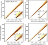 |
Fig. 5 Same as in Fig. 4, but for the predicted distributions of four output variables from the MDN trained on (M, R, T1) inputs. In view of the wide ranges of these four variables, a small chart is inserted for each output variable to illustrate the low-value behavior. Jupiter’s interior properties are marked by navy blue stars in the four inserted charts. |
Basic thermal parameters for Jupiter and Saturn (de Pater & Lissauer 2010).
Application to gas giants in the Solar System and gaseous giant exoplanets
We applied our trained MDN with (M, R, T1) inputs to four representative planets: gas giants in our Solar System and beyond. Meanwhile, the validation data sets for these four planets were generated using the above interior models and the uncertainties on the mass and radius were considered by introducing a standard deviation
![Mathematical equation: \begin{eqnarray*}\sigma=\sqrt{\big{[}(\Delta M/M)^{2}+(\Delta R/R)^{2}\big{]}\big{/}2},\end{eqnarray*}](/articles/aa/full_html/2022/02/aa42874-21/aa42874-21-eq10.png) (7)
(7)
where M and R are the actual values of planetary mass and radius, and ΔM and ΔR denote the deviations of one sample from the actual values.
Jupiter and Saturn, as gas giants in our Solar System, have been explored by various missions over the past 48 yr, providing strong constraints on their interior structures (Wahl et al. 2017; Guillot et al. 2018; Militzer et al. 2019). The basic thermal measurements of Jupiter and Saturn are given in Table 1. For direct comparison with the current interior model predictions (Wahl et al. 2017; Guillot et al. 2018; Ni 2019, 2020; Militzer et al. 2019; Nettelmann et al. 2021), the rotation periods of Jupiter and Saturn were separately fixed at 9 h 55 min 29.69s (Higgins et al. 1996) and 10 h 33 min 34 s (Militzer et al. 2019), and the standard deviation σ was restricted toa small value of 1% in the interior model calculations. The uncertainties on the surface temperatures T1 was also taken into account in the interior model calculations, where T1 was randomly varied between 160.0 and 170.0 K for Jupiter and between 130.0 and 140.0 K for Saturn. Figures 6 and 7 show the MDN predictions for Jupiter and Saturn using (M, R, T1) inputs, compared with the validation data set consisting of the interior model solutions. In particular, we would like to note that both MDN predictions and interior model solutions are confined to a very narrow area with respect to the whole range of interior properties. For the sake of clarity, we plotted the distributions of the interior properties within a very narrow range, although this creates the illusion of large derivations of the MDN predictions from the interior model solutions. In order to examine whether theMDN is capable of describing the thermal effect on planetary interiors, we paid special attention to T1 in the MDN predictions. Three different T1 inputs of 160, 165, and 170 K were chosen for Jupiter with the mass and radius inputs unchanged and three different T1 inputs of 130, 135, and 140 K for Saturn. The higher surface temperature T1 seems to allow a larger amount of heavy elements in the planetary interior. This is quite consistent with the interior model results of Ni (2019). Also, as the surface temperature is increased, the MDN predictions move toward an area of larger Tint and hotter TCEB.
Various interior models with new ingredients have been constructed to interpret the measured gravity data of Jupiter and Saturn. All interior models are dependent on the EOS of hydrogen and helium. Ni (2019) adopted different EOSs including CMS19 in four-layer structure calculations and investigated the effect of dilute cores on Jupiter’s interior. The CMS19 adiabat generally has a higher density (pressure) in the Mbar region with respect to the EOSs of Militzer & Hubbard (2013) and Saumon et al. (1995) (Chabrier et al. 2019). This would bring in a lower planetary metallicity for CMS19. Indeed, the results of CMS19 yield Jupiter’s total heavy-element mass over a narrow range of 8–12 M⊕, showing the lowest global metallicity among four EOSs (Ni 2019). Militzer et al. (2019) explored Saturn’s interior from the Cassini Grand Finale gravity measurements using the MH13+SCvH EOS, where Saturn’s heavy-element mass is predicted as 16.5–23 M⊕. Ni (2020) discussed the internal structure and interior composition of Saturn within the four-layer structure model using REOS3b and MH13+SCvH, where the MH13+SCvH solutions yield Saturn’s heavy-element mass of 16–19 M⊕. With respect to the MH13+SCvH results, the models using CMS19 are expected to allow a smaller amount of heavy elements. That is, the CMS19 solutions would yield Saturn’s total heavy-element mass of roughly or less than 16 M⊕. Very recently Nettelmann et al. (2021) have investigated the interiors of Jupiter and Saturn using the CMS19 H–He EOS, suggesting the heavy-element masses of 7.5–10.1 M⊕ and 12.6–13.6 M⊕ for Jupiter and Saturn. For comparison, the CMS19 results for the total heavy-element masses of Jupiter and Saturn, which were determined from the detailed interior models of Ni (2019) and Nettelmann et al. (2021), are also shown in Figs. 6 and 7. One can see that the MDN predictions of MZ not only show good agreement with the validation data set within the error allowed, but also follow the other detailed interior models of Jupiter and Saturn (Nettelmann et al. 2021; Militzer et al. 2019; Ni 2019, 2020). There is an overestimation of Tint, PCEB, and TCEB for the MDN predictions, as discussed in the previous subsection. This overestimation can be neglected as compared with the systematic error because these quantities are varied by several orders of magnitude. Based on the thermal measurements listed in Table 1, the intrinsic temperatures of Jupiter and Saturn are derived from Eq. (6) as 98.2 K and 78.7 K, respectively. The MDN predictions of Tint cover these two values. The MDN predictions of PCEB and TCEB are also consistent with the four-layer interior models of Ni (2019, 2020).
For gaseous giant exoplanets, we consider CoRoT-9b as a Jupiter-sized representative and CoRoT-6b as a hot Jupiter representative. Observational data of these two exoplanets have been provided by several groups as summarizedbelow. Deeg et al. (2010) determined the absolute values for CoRoT-9b’s mass and radius as M = 0.84 ± 0.07MJ and R = 1.05 ± 0.04 Jupiter radii (RJ) and gave anirradiation temperature between 250 K and 430 K. Bonomo et al. (2017) performed a Bayesian combined analysis of photometric observations from the CoRoT and Spitzer space telescopes and five-year spectroscopic monitoring with HARPS. They obtained the best values for CoRoT-9b’s mass, radius, and equilibrium temperature as M = 0.84 ± 0.05 MJ,  RJ, and Teq = 420 ± 16 K. Fridlund et al. (2010) analyzed the photometric light curve from the CoRoT telescope as well as the photometric and spectroscopic ground-based follow-up observations, resulting in the physical properties of CoRoT-6b as M = 2.96 ± 0.34MJ, R = 1.166 ± 0.035RJ, and Teq = 1017 ± 19 K. Southworth (2011) also derived the physical properties of CoRoT-6b using homogeneous methods and by combining all available photometric data with measured spectroscopic parameters of host stars, M = 2.96 ± 0.39MJ, R = 1.185 ± 0.050RJ, and Teq = 1025 ± 16 K, covering the previous findings of Fridlund et al. (2010). At present, there is little knowledge of surface temperatures for CoRoT-9b and CoRoT-6b. And, furthermore, the equilibrium temperature Teq of a planet is neither an upper nor lower bound to its surface temperature (Guillot 2005). Considering the effects of the surface temperatures on interior properties had been illustrated in Figs. 6 and 7, we roughly assume the surface temperatures T1 of CoRoT-9b and CoRoT-6b to be equal to their equilibrium temperature Teq. Figures 8 and 9 show the MDN predictions for CoRoT-9b and CoRoT-6b using (M, R, T1) inputs to the MDN, compared with the validation data set with the standard deviation σ = 3%. As one can see, the distributions of the interior properties are restricted into a narrow range. In both cases, the MDN predictions show good agreement with the interior model solutions, especially for CoRoT-6b.
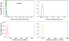 |
Fig. 6 MDN predictions of the interior properties for Jupiter. Colored lines denote the combined Gaussian mixture prediction from the MDN with (M, R, T1) inputs, where different shades of color correspond to different surface temperatures (T1 = 160, 165, 170 K from light to dark). Shaded areas denote the validation results from the interior models with the standard deviation σ = 1%. As additional information, Jupiter’s total heavy-element mass, determined from the detailed interior models using the CMS19 H–He EOS as well (Ni 2019; Nettelmann et al. 2021), is shown by green vertical bands. |
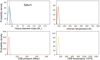 |
Fig. 7 Same as in Fig. 6, but for Saturn. For the MDN predictions denoted by colored lines, different shades of color correspond to different surface temperatures (T1 = 130, 135, 140 K from light to dark). Saturn’s total heavy-element mass, determined from the detailed interior models using the CMS19 H–He EOS as well (Nettelmann et al. 2021), is shown by green vertical bands. |
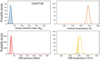 |
Fig. 8 MDN predictions of the interior properties for CoRoT-9b. Colored lines denote the combined Gaussian mixture prediction from the MDN with (M, R, T1) inputs. Shaded areas denote the validation results from the interior models with the standard deviation σ = 3%. |
5 Summary
As an extension of the previous work for rocky exoplanets (Zhao & Ni 2021), we applied MDN techniques to infer the interior properties of gaseous giant exoplanets with 0.1 MJ < M < 10 MJ. Compared with the case of rocky exoplanets, the crucial difficulty for gas giant exoplanets is that they show larger diversities in thermal states and their interior properties span over a much wider range by several orders of magnitude. We developed two-layer interior models using the H–He–rock–ice EOSs and generated sufficient data samples by solving the interior models with various physical parameters. The data were then trained based on two MDN models and the resulting MDNs are available on GitHub1. The interior properties of a planet, as MDN output variables, contain the total heavy-element mass in planetary interior MZ, the intrinsic effective temperatureTint, and the pressure PCEB and temperature TCEB at the CEB. The MDN trained on mass and radius inputs only works in predicting the pressure PCEB, but this yields the large degeneracy of the other interior properties in particular for MZ, as shown in Fig. 4. Using the temperature at the 1-bar level T1 as additional input, the new MDN shows good performance in predicting the interior properties of gas giant exoplanets, as shown in Fig. 5. This suggests that the surface temperature is necessary to characterize the interior of gas giant exoplanets owing to their large diversities in thermal states. In spite of the difficulties mentioned above, the MDN can be efficiently trained for gaseous giant exoplanets to bypass the interior model calculations. We also applied the well-trained MDN to our Solar System giants (Jupiter and Saturn) and two representative gas giants (CoRoT-9b and CoRoT-6b). For Jupiter and Saturn, the MDN predictions are not only in good agreement with the validation data set, but also consistent with the more sophisticated interiors models of Militzer et al. (2019), Ni (2019, 2020), and Nettelmann et al. (2021). The trained MDN is also found to work well for CoRoT-9b and CoRoT-6b, as shown in Figs. 8 and 9. The MDN offers a convenient and powerful tool for quick knowledge of the interiorsof gaseous giant exoplanets and hence more insight into planet formation in diverse protoplanetary environments.
Acknowledgements
This work is supported by the National Natural Science Foundation of China (Grant No. 12022517), the Science and Technology Development Fund, Macau SAR (File No. 0048/2020/A1 and 0002/2019/APD), and the Pre-Research Projects on Civil Aerospace Technologies of China National Space Administration (Grant No. D020308 and D020303).
References
- Abadi, M., Barham, P., Chen, J., et al. 2016, Tensorflow: A system for large-scale machine learning [arXiv:1605.08695] [Google Scholar]
- Adibekyan, V., Dorn, C., Sousa, S. G., et al. 2021, Science, 374, 330 [NASA ADS] [CrossRef] [Google Scholar]
- Alibert, Y., & Venturini, J. 2019, A&A, 626, A21 [NASA ADS] [CrossRef] [EDP Sciences] [Google Scholar]
- Atkins, C., Valentine, A. P., Tackley, P. J., & Trampert, J. 2016, Phys. Earth Planet. Inter., 257, 171 [CrossRef] [Google Scholar]
- Batalha, N. M. 2014, PNAS, 111, 12647 [NASA ADS] [CrossRef] [Google Scholar]
- Baumeister, P., Padovan, S., Tosi, N., Montavon, G., & Nettelmann, N. 2020, ApJ, 889, 42 [NASA ADS] [CrossRef] [Google Scholar]
- Bishop, C. M. 1994, Mixture Density Networks, Tech. Rep. NCRG/94/004 [Google Scholar]
- Bonomo, A. S., Hébrard, G., Raymond, S. N., et al. 2017, A&A, 603, A43 [NASA ADS] [CrossRef] [EDP Sciences] [Google Scholar]
- Boujibar, A., Driscoll, P., & Fei, Y. 2020, J. Geophys. Res. Planets, 125, e2019JE006124 [CrossRef] [Google Scholar]
- Brugger, B., Mousis, O., Deleuil, M., & Deschamps, F. 2017, ApJ, 850, 93 [NASA ADS] [CrossRef] [Google Scholar]
- Brygoo, S., Loubeyre, P., Millot, M., et al. 2021, Nature, 593, 517 [NASA ADS] [CrossRef] [Google Scholar]
- Chabrier, G., Mazevet, S., & Soubiran, F. 2019, ApJ, 872, 51 [NASA ADS] [CrossRef] [Google Scholar]
- Chollet, F., et al. 2015, Keras: The Python Deep Learning library, https://keras.io [Google Scholar]
- de Pater, I., & Lissauer, J. J 2010, Planetary Sciences (Cambridge: Cambridge University Press) [CrossRef] [Google Scholar]
- Debras, F., & Chabrier, G. 2019, ApJ, 872, 100 [Google Scholar]
- Deeg, H. J., Moutou, C., Erikson, A., et al. 2010, Nature, 464, 384 [NASA ADS] [CrossRef] [Google Scholar]
- Dorn, C., Khan, A., Heng, K., et al. 2015, A&A, 577, A83 [NASA ADS] [CrossRef] [EDP Sciences] [Google Scholar]
- Dorn, C., Venturini, J., Khan, A., et al. 2017, A&A, 597, A37 [NASA ADS] [CrossRef] [EDP Sciences] [Google Scholar]
- Fortney, J. J., Marley, M. S., & Barnes, J. W. 2007, ApJ, 659, 1661 [Google Scholar]
- Fortney, J. J., Ikoma, M., Nettelmann, N., Guillot, T., & Marley, M. S. 2011, ApJ, 729, 32 [NASA ADS] [CrossRef] [Google Scholar]
- Fortney, J. J., Dawson, R. I., & Komacek, T. D. 2021, J. Geophys. Res. Planets, 126, e2020JE006629 [CrossRef] [Google Scholar]
- Fridlund, M., Hébrard, G., Alonso, R., et al. 2010, A&A, 512, A14 [NASA ADS] [CrossRef] [EDP Sciences] [Google Scholar]
- Goodfellow, I., Bengio, Y., & Courville, A. 2016, Deep Learning (Cambridge: MIT Press) [Google Scholar]
- Guillot, T. 2005, Annu. Rev. Earth Planet. Sci., 33, 493 [Google Scholar]
- Guillot, T., & Showman, A. P. 2002, A&A, 385, 156 [NASA ADS] [CrossRef] [EDP Sciences] [Google Scholar]
- Guillot, T., Miguel, Y., Militzer, B., et al. 2018, Nature, 555, 227 [Google Scholar]
- Higgins, C. A., Carr, T. D., & Reyes, F. 1996, Geophys. Res. Lett. 23, 2653 [NASA ADS] [CrossRef] [Google Scholar]
- Kingma, D. P., & Ba, J. 2014, ArXiv e-prints [arXiv:1412.6980] [Google Scholar]
- Kramm, U., Nettelmann, N., Fortney, J. J., Neuhäuser, R., & Redmer, R. 2012, A&A, 538, A146 [NASA ADS] [CrossRef] [EDP Sciences] [Google Scholar]
- Leconte, J., & Chabrier, G. 2013, NatGe, 6, 347 [NASA ADS] [Google Scholar]
- Mankovich, C.R., & Fortney, J. J. 2020, ApJ, 889, 51 [NASA ADS] [CrossRef] [Google Scholar]
- Marley, M. S., Fortney, J., Seager, S., & Barman, T. 2007, in Protostars and Planets V, eds. B. Reipurth, D. Jewitt, & K. Keil, 733 [Google Scholar]
- Martin, C., & Duhaime, D. 2019, https://doi.org/10.5281/zenodo.2578015 [Google Scholar]
- Montavon, G., Orr, G., & Müller, K.-R. 2012, Neural networks-tricks of the trade 2nd ed. (Springer) [CrossRef] [Google Scholar]
- Militzer, B., & Hubbard, W. B. 2013, ApJ, 774, 148 [NASA ADS] [CrossRef] [Google Scholar]
- Militzer, B., Wahl, S., & Hubbard, W. B. 2019, ApJ, 879, 78 [Google Scholar]
- Nettelmann, N., Kramm, U., Redmer, R., Neuhäuser, R. 2010, A&A, 523, A26 [NASA ADS] [CrossRef] [EDP Sciences] [Google Scholar]
- Nettelmann, N., Movshovitz, N., Ni, D., et al. 2021, PSJ, submitted [Google Scholar]
- Ni, D. 2019, A&A, 632, A76 [NASA ADS] [CrossRef] [EDP Sciences] [Google Scholar]
- Ni, D. 2020, A&A, 639, A10 [NASA ADS] [CrossRef] [EDP Sciences] [Google Scholar]
- Pedregosa, F., Varoquaux, G., Gramfort, A., et al. 2011, J. Mach. Learn. Res., 12, 2825 [Google Scholar]
- Rogers, L. A., & Seager, S. 2010, ApJ, 712, 974 [Google Scholar]
- Saumon, D., Chabrier, G., & van Horn, H. M. 1995, ApJS, 99, 713 [NASA ADS] [CrossRef] [Google Scholar]
- Schöttler, M., & Redmer, R. 2018, Phys. Rev. Lett., 120, 115703 [CrossRef] [Google Scholar]
- Serenelli, A. M., & Basu, S. 2010, ApJ, 719, 865 [NASA ADS] [CrossRef] [Google Scholar]
- Sotin, C., Grasset, O., & Mocquet, A. 2007, Icarus, 191, 337 [Google Scholar]
- Southworth, J. 2011, MNRAS, 417, 2166 [Google Scholar]
- Spiegel, D. S., Fortney, J. J., & Sotin, C. 2014, PNAS, 111, 12622 [NASA ADS] [CrossRef] [Google Scholar]
- Srivastava, N., Hinton, G., Krizhevsky, A., Sutskever, I., & Salakhutdinov, R. 2014, J. Mach. Learn. Res., 15, 1929 [Google Scholar]
- Thompson, S. L. 1990, ANEOS Analytic Equations of State for Shock Physics Codes Input Manual, Tech. Rep., (Albuquerque, NM: Sandia National Laboratories [Google Scholar]
- Thorngren, D. P., Fortney, J. J., Murray-Clay, R. A., & Lopez, E. D. 2016, ApJ, 831, 64 [NASA ADS] [CrossRef] [Google Scholar]
- Ulmer-Moll, S., Santos, N. C., Figueira, P., Brinchmann, J., & Faria, J. P. 2019, A&A, 630, A135 [NASA ADS] [CrossRef] [EDP Sciences] [Google Scholar]
- Valencia, D., Sasselov, D. D., & O’Connell, R. J. 2007, ApJ, 665, 1413 [Google Scholar]
- Wahl, S. M., Hubbard, W. B., Militzer, B., et al. 2017, Geophys. Res. Lett., 44, 4649 [CrossRef] [Google Scholar]
- Zhao, Y., & Ni, D. 2021, A&A, 650, A177 [NASA ADS] [CrossRef] [EDP Sciences] [Google Scholar]
- Zhao, Y., Zhang, Y., Geng, M., Jiang, J., & Zou, X. 2019, Geophys. Res. Lett., 46, 5234 [NASA ADS] [CrossRef] [Google Scholar]
All Tables
All Figures
|
Fig. 1 Schematic interior structure of gaseous giant exoplanets. The compact core with mass Mcore is characterized by the pressure and temperature at the core envelope boundary (CEB), PCEB and TCEB. The surface defined by the 1-bar pressure level is characterized by the temperature T1 bar and the deeper atmosphere at the 10-bar pressure level by the temperature T10 bar. |
| In the text | |
|
Fig. 2 Sketch map of the mixture density network (MDN) where Gaussian mixture models are combined with the neural network. Three hidden layers are involved in the neutral network and each layer has 512 neurons. Twenty Gaussian mixture components are involved in the mixture model and each component is characterized by means μ, variances σ2, and mixing coefficients α. |
| In the text | |
|
Fig. 3 Negative log-likelihood (NLL) loss for the MDN model trained on mass and radius inputs only and for the MDN model trained on mass, radius, and T1 inputs. (a) Dependence of the NLL loss on the size of the training data set for the two MDN models. (b) Learning curve of the MDN trained on mass and radius inputs only for both the training and validation data sets. (c) Learning curve of the MDN trained on mass, radius, and T1 inputs for both the training and validation data sets. |
| In the text | |
|
Fig. 4 Predicted distributions of four output variables from the MDN trained on (M, R) inputs versus the actual values obtained from the interior models for the testing data set: total heavy-element mass MZ, intrinsic effective temperature Tint, as well as pressure and temperature at the core envelope boundary (CEB), PCEB and TCEB. Blue dasheddiagonal lines denote a perfect performance of the MDN. The predicted distributions are colored according to the local probability density (the color scale is black at the maximum). |
| In the text | |
|
Fig. 5 Same as in Fig. 4, but for the predicted distributions of four output variables from the MDN trained on (M, R, T1) inputs. In view of the wide ranges of these four variables, a small chart is inserted for each output variable to illustrate the low-value behavior. Jupiter’s interior properties are marked by navy blue stars in the four inserted charts. |
| In the text | |
|
Fig. 6 MDN predictions of the interior properties for Jupiter. Colored lines denote the combined Gaussian mixture prediction from the MDN with (M, R, T1) inputs, where different shades of color correspond to different surface temperatures (T1 = 160, 165, 170 K from light to dark). Shaded areas denote the validation results from the interior models with the standard deviation σ = 1%. As additional information, Jupiter’s total heavy-element mass, determined from the detailed interior models using the CMS19 H–He EOS as well (Ni 2019; Nettelmann et al. 2021), is shown by green vertical bands. |
| In the text | |
|
Fig. 7 Same as in Fig. 6, but for Saturn. For the MDN predictions denoted by colored lines, different shades of color correspond to different surface temperatures (T1 = 130, 135, 140 K from light to dark). Saturn’s total heavy-element mass, determined from the detailed interior models using the CMS19 H–He EOS as well (Nettelmann et al. 2021), is shown by green vertical bands. |
| In the text | |
|
Fig. 8 MDN predictions of the interior properties for CoRoT-9b. Colored lines denote the combined Gaussian mixture prediction from the MDN with (M, R, T1) inputs. Shaded areas denote the validation results from the interior models with the standard deviation σ = 3%. |
| In the text | |
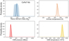 |
Fig. 9 Same as in Fig. 8, but for CoRoT-6b. |
| In the text | |
Current usage metrics show cumulative count of Article Views (full-text article views including HTML views, PDF and ePub downloads, according to the available data) and Abstracts Views on Vision4Press platform.
Data correspond to usage on the plateform after 2015. The current usage metrics is available 48-96 hours after online publication and is updated daily on week days.
Initial download of the metrics may take a while.