| Issue |
A&A
Volume 693, January 2025
|
|
|---|---|---|
| Article Number | L7 | |
| Number of page(s) | 7 | |
| Section | Letters to the Editor | |
| DOI | https://doi.org/10.1051/0004-6361/202452783 | |
| Published online | 03 January 2025 | |
Letter to the Editor
Giant exoplanet composition
The impact of the hydrogen–helium equation of state and interior structure
Institut für Astrophysik, Universität Zürich, Winterthurerstr. 190, CH8057 Zurich, Switzerland
⋆ Corresponding author; This email address is being protected from spambots. You need JavaScript enabled to view it.
Received:
28
October
2024
Accepted:
4
December
2024
Abstract
Context. Revealing the internal composition and structure of giant planets is fundamental for understanding planetary formation. However, the bulk composition can only be inferred through interior models. As a result, advancements in modelling aspects are essential to better characterise the interiors of giant planets.
Aims. We investigate the effects of model assumptions such as the interior structure and the hydrogen–helium (H–He) equation of state (EOS) on the inferred interiors of giant exoplanets.
Methods. We first assessed these effects on a few test cases and compared H–He EOSs. We then calculated evolution models and inferred the planetary bulk metallicity of 45 warm exoplanets, ranging from 0.1 to 10 MJ.
Results. Planets with masses between about 0.2 and 0.6 MJ are most sensitive to the H–He EOS. Using a H–He EOS that properly models the warm dense matter regime reduces the inferred heavy-element mass, with an absolute difference in bulk metallicity of up to 13%. Concentrating heavy elements in a core, rather than distributing them uniformly (and scaling opacities with metallicity), reduces the inferred metallicity (up to 17%). The assumed internal structure, along with its effect on the envelope opacity, has the greatest effect on the inferred composition of massive planets (Mp > 4 MJ). For Mp > 0.6 MJ, the observational uncertainties on radii and ages lead to uncertainties in the inferred metallicity (up to 31%) that are larger than the ones associated with the used H–He EOS and the assumed interior structure. However, for planets with 0.2 < Mp < 0.6 MJ, the theoretical uncertainties are larger.
Conclusions. Advancements in EOSs and our understanding of giant planet interior structures combined with accurate measurements of the planetary radius and age are crucial for characterising giant exoplanets.
Key words: planets and satellites: composition / planets and satellites: gaseous planets / planets and satellites: interiors
© The Authors 2025
 Open Access article, published by EDP Sciences, under the terms of the Creative Commons Attribution License (https://creativecommons.org/licenses/by/4.0), which permits unrestricted use, distribution, and reproduction in any medium, provided the original work is properly cited.
This article is published in open access under the Subscribe to Open model. This email address is being protected from spambots. You need JavaScript enabled to view it. to support open access publication.
1. Introduction
Determining the bulk composition and internal structure of giant planets is fundamental for understanding their origin (e.g. Mordasini et al. 2016; Turrini et al. 2018). Observations of giant exoplanets have advanced significantly, enabling measurements of the planetary mass and radius and, in a few cases, also of the atmospheric composition (e.g. Kreidberg et al. 2014; Madhusudhan et al. 2014; Edwards et al. 2023). However, the bulk composition of giant exoplanets is typically inferred through models, where the planetary structure is constrained by mass, radius, and age measurements.
Accurate measurements of the gravitational fields and atmospheric composition of Jupiter and Saturn have led to the development of a more comprehensive theoretical framework for giant planet modelling. Interior models of both Jupiter and Saturn that fit Juno (Bolton et al. 2017) and Cassini (Spilker 2019) data suggest that the planets have dilute cores and complex interiors (Wahl et al. 2017; Mankovich & Fuller 2021; Miguel et al. 2022; Howard et al. 2023a; Helled & Stevenson 2024; Howard et al. 2023b; Müller & Helled 2024). In addition, giant planet models rely on our understanding of the hydrogen–helium equation of state (H–He EOS). Progress from the semi-analytical EOS of Saumon et al. (1995) to ab initio simulations (e.g. Militzer & Hubbard 2013) has led to more accurate modelling of the warm dense matter regime where dissociation and pressure ionisation occur and H–He interactions are important.
As observational uncertainties are progressively being reduced, thanks to ground-based observations (e.g. HARPS; Mayor et al. 2003, NIRPS; Bouchy et al. 2017, ESPRESSO; Pepe et al. 2021) and space missions (e.g. Kepler; Borucki et al. 2010, TESS; Ricker et al. 2015, JWST; Gardner et al. 2006 and in the future PLATO; Rauer et al. 2014 and Ariel; Tinetti et al. 2018), it is clear that more advanced models should be used for the characterisation of giant exoplanets. In addition, it is important to identify the theoretical uncertainties and compare them to the observational ones.
Several previous studies have explored the importance of model assumptions such as the interior structure and the EOS on the inferred planetary bulk composition (Baraffe et al. 2008; Müller et al. 2020; Bloot et al. 2023). The large sample of observed giant exoplanets with a measured radius, mass, and age can be combined with theoretical models to infer the relationship between the planetary mass and its metallicity (Thorngren et al. 2016; Müller & Helled 2023). The goal of this work is to further investigate the effects of model assumptions on the inferred internal structures of giant exoplanets. Our models use the most up-to-date H–He EOS, allow for ‘core+envelope’ and ‘fully mixed’ interiors, and account for the opacity’s dependence on the metallicity. Our paper is organised as follows. Section 2 describes our methods. In Sect. 3 we analyse the effects of the assumed interior structure and H–He EOS on a few test cases. Section 4 focuses on a sample of observed exoplanets. Our conclusions are presented in Sect. 5.
2. Methods
We used CEPAM (Guillot & Morel 1995; Howard et al. 2024) to run planetary evolution models and assess the effects of both the H–He EOS and the assumed interior structure (i.e. the distribution of heavy elements). We compared calculations using the SCvH95 (Saumon et al. 1995) (which is still used (e.g. Thorngren et al. 2016) and the CMS19+HG23 EOSs (Chabrier et al. 2019; Howard & Guillot 2023). More details about the differences between these EOSs are presented in Sect. 3. We also compared models assuming either a ‘core+envelope’ or ‘fully mixed’ structure. In the first structure, all the heavy elements were concentrated in a central core. We used the analytical EOS of Hubbard & Marley (1989) to calculate the pressure-dependent density in the isothermal core, which was assumed to be made up of 50% ices and 50% rocks. In the second structure, the heavy elements were uniformly distributed within the planet. We also assumed an ice-to-rock ratio of unity and used the SESAME water EOS for ices and the SESAME drysand EOS for rocks (Lyon & Johnson 1992). The hydrogen-to-helium ratio in the envelope was protosolar: Y/(X + Y) = 0.27 (Asplund et al. 2021). Our models used a non-grey atmosphere (Parmentier et al. 2015) and the method from Valencia et al. (2013) to account for the opacity enhancement due to the heavy elements. An increase in the opacity in the radiative atmosphere can slow the planetary cooling (Guillot 2005).
3. Proof of concept: Metallicities of synthetic giant planets
We first calculated models of synthetic planets, with masses of 0.3, 1 and 3 MJ. We focused on planets that are not highly irradiated and hence not inflated (e.g. Thorngren & Fortney 2018; Fortney et al. 2021), with an equilibrium temperature Teq of 500 K. For each planetary mass, we ran models with both H–He EOSs (SCvH95 and CMS19+HG23) and internal structures (core+envelope and fully mixed). We assumed different bulk metallicities Z, from 0 to 0.5 (Z = MZ/Mp where MZ and Mp are the heavy-element mass and the planet’s mass, respectively).
Figure 1 shows the planetary radius versus time for the different cases. For the core+envelope structure, CMS19+HG23 always yields smaller radii than SCvH95, by up to 10% (Müller et al. 2020 found that CMS19 also yields smaller radii). We also find that higher metallicities lead to smaller radii. The range of radii spanned by models with different metallicities is larger for lower-mass planets. For Mp = 0.3 MJ, the radius decreases by about a factor of two when changing Z from 0 to 0.25; whereas, for Mp = 3 MJ, changing Z from 0 to 0.5 changes the radius by only 15%. For a given measured radius and its associated uncertainty, the range of inferred metallicity is narrower for a 0.3 MJ planet compared to a 3 MJ planet. In addition, for a given measured radius and its uncertainty, the core+envelope structure leads to a narrower range of inferred metallicity for a 0.3 MJ planet, compared to a fully mixed structure. However, the opposite behaviour is expected for a 3 MJ planet. The comparison between both structures depends on the planetary mass and metallicity.
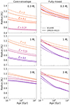 |
Fig. 1. Radius vs. time for planets with masses of 0.3, 1, and 3 MJ (top, middle, and bottom panels, respectively). Left (right) panels correspond to models assuming a core+envelope (fully mixed) structure. Results with different H–He EOSs are shown with dashed and solid lines. The colours correspond to different assumed metallicities. The middle and bottom panels have similar limits on the y-axis, but not the top panels. |
In the fully mixed case, higher metallicities do not always lead to smaller radii. This is because of two opposite effects due to enriching the envelope with heavy elements: it increases both the mean molecular weight and the opacities (Guillot 2005). At early times, the opacity effect dominates and delays the cooling and contraction of the planet; however, at late times, the mean molecular weight effect prevails. Müller et al. (2020) also found that the radius does not monotonically decrease with Z if the effect of the heavy elements on the opacity is accounted for. For Mp = 0.3 MJ, we find that CMS19+HG23 always yields smaller radii than SCvH95. However, this is not the case for Mp = 1 and 3 MJ. For these two planetary masses, especially at early times, CMS19+HG23 yields larger radii than SCvH95 for Z > 0.
Understanding these results requires investigating the differences between the SCvH95 and CMS19+HG23 EOSs. SCvH95 is based on the so-called chemical picture (see Saumon et al. 1995, for a detailed description). It models the interactions between molecules or atoms by using pair potentials. The Helmholtz-free energy is determined through the free-energy minimisation technique and pressure, entropy, or internal energy can then be calculated (Hummer & Mihalas 1988). However, at densities corresponding to dissociation and pressure ionisation, pair potentials fail at correctly describing describing the behaviour of matter. Using the additive volume law, one can combine pure H and He tables to obtain the properties (density and entropy at given pressures and temperatures) of a H–He mixture. On the other hand, CMS19+HG23 also applies the additive volume law using pure H and He tables from Chabrier et al. (2019), while additionally accounting for non-ideal mixing effects as described by Howard & Guillot (2023). It combines different EOS calculations: it is based on SCvH95 in the low density regime and on a fully ionised model in the high density regime. In the intermediate regime, it uses the ab initio data from Militzer & Hubbard (2013). Based on the physical picture, these ab initio calculations focus on electrons and nuclei and model their interactions by Coulomb potentials. Considering a H–He mixture (in proportions close to protosolar), Militzer & Hubbard (2013) provided a more realistic description of the regime of dissociation and ionisation and inherently a better incorporation of H–He interactions.
Figure 2 shows the relative difference in density between CMS19+HG23 and SCvH95. We include the T–P profiles of some models from Fig. 1, at 0.1 and 10 Gyr. We calculated the differences assuming a H–He mixture of protosolar composition (He mass fraction of Y = 0.27), and interpolated the density from CMS19+HG23 at the pressure and temperature points corresponding to SCvH95. In the region where ab initio calculations from Militzer & Hubbard (2013) have been performed (dotted black square), the T–P profiles of our models can go through regions where CMS19+HG23 is denser than SCvH95 (shown in blue) or less dense (shown in red). We note that entropy influences a planet’s position on the T–P diagram by affecting the calculation of the adiabatic gradient. The density differences between the EOSs under these T–P conditions then explain the differences in inferred planetary radii.
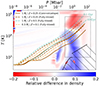 |
Fig. 2. Relative difference in density between the CMS19+HG23 (Chabrier et al. 2019; Howard & Guillot 2023) and SCvH95 (Saumon et al. 1995) EOSs. Blue regions on the T–P diagram indicate where CMS19+HG23 is denser than SCvH95, while red regions highlight less dense areas. The coloured solid and dashed lines show T–P profiles of some models (using CMS19+HG23) from Fig. 1, at 0.1 or 10 Gyr. The dotted square indicates the region of the ab initio presented by Militzer & Hubbard (2013). The CMS19+HG23 EOS is more accurate in this region. The hashed area corresponds to the region where hydrogen becomes solid (see e.g. Chabrier et al. 2019). |
We find that 1 MJ with Z = 0.25 and a core+envelope structure (solid brown line) mostly covers the region where CMS19+HG23 is denser than SCvH95 (around 1 Mbar). Interestingly, we find that the T–P profiles of models assuming the core+envelope structure are rather similar even when the planetary mass or metallicity are changed. Hence, we find that CMS19+HG23 yielded smaller radii compared to SCvH95 in the core+envelope case, regardless of planetary mass and metallicity (see left panels of Fig. 1). However, T–P profiles of fully mixed models are more affected by changing the mass and metallicity. These models have a much hotter interior because enhancing the opacities due to heavy-element enrichment in the envelope delays the planetary cooling. The 0.3 MJ model shown in Fig. 2 (dashed orange line) is still in a T–P regime where CMS19+HG23 is denser than SCvH95, explaining why CMS19+HG23 yielded smaller radii than SCvH95 for Mp = 0.3 MJ in the fully mixed case (see top right panel of Fig. 1). The 1 MJ model with Z = 0.25 (dashed brown line) goes through the less dense region at 0.1 Gyr but is then mostly affected by the denser region at 10 Gyr. This explains why CMS19+HG23 yielded larger radii at early times and smaller radii at late times (middle right panel of Fig. 1). Overall, the differences in radii between CMS19+HG23 and SCvH95 seen in Fig. 1 depend on the position of the planet within the temperature–pressure–density space during its evolution. As CMS19+HG23 models the regime of dissociation and ionisation more accurately, this H–He EOS should be used for exoplanet characterisation.
4. Inferred metallicities of observed giant exoplanets
In this section we characterise a sample of observed giant exoplanets. We used the PlanetS catalogue (Otegi et al. 2020; Parc et al. 2024) and selected planets with masses from 0.1 to 10 MJ with relative measurement uncertainties smaller than 10 and 8% for the mass and radius, respectively. We selected planets with Teq < 1000 K and with an age estimate. Our sample consists of 45 exoplanets (listed in Appendix A) that allowed for a reliable determination of the internal composition.
For each exoplanet, we inferred the heavy-element mass (MZ) by calculating two evolution models, which fit the upper and lower bounds of the radius and age measurements ( and
and  , listed in Table A.1). This provided the possible range of the inferred bulk metallicity (Zp = MZ/Mp). The mass uncertainty was not considered. The inferred heavy-element mass for our sample of exoplanets is shown in Fig. 3 (top panels). We also show the absolute difference in the inferred heavy-element mass (ΔMZ) between both EOSs (middle panels) as well as the absolute difference in the bulk metallicity (ΔZp = ΔMZ/Mp) (bottom panels).
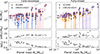 |
Fig. 3. Inferred heavy-element mass vs. planetary mass. Top panels: comparison of the results obtained with CMS19+HG23 and SCvH95, for both core+envelope and fully mixed structures. The circles represent the midpoint between the upper and lower bounds of the errorbars. Middle panels: absolute difference in heavy-element mass due to the H–He EOS update. Bottom panels: absolute difference in bulk metallicity. Empty circles correspond to planets for which CMS19+HG23 leads to a higher metallicity than SCvH95. The dotted black line shows the 1/Mp curve. |
For the core+envelope case, we find the following: (i) CMS19+HG23 yields a lower heavy-element mass than SCvH95 for all planets; (ii) ΔMZ increases with Mp in the range from Mp = 0.1 MJ to Mp = 1 MJ, after which it reaches a plateau at ΔMZ ∼ 15 M⊕ for planets with masses larger than 1 MJ; and (iii) ΔZp peaks at Mp = 0.3 MJ, with a value of ∼11%. In the fully mixed case, we find that: (i) CMS19+HG23 also yields a lower heavy-element mass than SCvH95 except for six planets. This includes the two most massive planets from our sample, as expected (see Sect. 3). (ii) The variation of ΔMZ is similar to the core+envelope case. However, there is greater scatter from Mp > 1 MJ. Lastly, (iii) ΔZp peaks at Mp = 0.4 MJ, with a maximum value of about 13%.
We find that the inferred bulk metallicity of planets with masses between 0.2 and 0.6 MJ is most affected by the H–He EOS update. This holds for both interior structures and the absolute difference in bulk metallicity can go up to 13%. This is due to how the planets lie in the temperature–pressure–density space (Fig. 2). Planets with Mp < 0.2 MJ are less affected by changing the H–He EOS as they only have a small amount of H–He. We also note that CMS19+HG23 leads to eight additional planets (compared to SCvH95) for which the lower limit of the inferred heavy element mass is zero (in Table A.1, planets with a single dagger). For these planets, the radius inferred from a pure H–He model cannot match the upper bound of the measured radius suggesting that these planets may be inflated.
We subsequently compared the heavy-element content obtained with the core+envelope and fully mixed structures, using CMS19+HG23. We show the mass–metallicity relation by calculating the ratio of the planet metallicity Zplanet to that of the parent star Zstar. We followed Müller & Helled (2023) and performed a Bayesian linear regression. The parameters α and β of the power-law Zplanet/Zstar = β × M[MJ]α were estimated using a Markov chain Monte Carlo method and their posterior distributions are shown in Appendix B. Figure 4 (top panel) shows the best fit as well as the 1σ error contour for both structures.
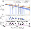 |
Fig. 4. Mass–metallicity relation with both interior structures, using the CMS19+HG23 EOS. Top panel: errorbars show the inferred range of bulk metallicity with the core+envelope (blue) or fully mixed (orange) structure, as in Fig. 3. Orange and blue lines show the best fit for both cases, while the shaded areas show the 1σ error contour. The metallicities of Jupiter and Saturn (Helled & Howard 2024) are shown in black. The solid and dashed grey lines show the best fits from Müller & Helled (2023) and Thorngren et al. (2016), respectively. The star metallicities were derived using the solar value from Asplund et al. (2021). Middle panel: absolute difference in metallicity due to either the H–He EOS (grey dots, taken from Fig. 3) or the interior structure (squares). Blue (orange) squares indicate planets where the core+envelope case gives lower (higher) metallicity than the fully mixed case. Bottom panel: absolute difference in metallicity. Pink dots show the sum of the H–He EOS and the interior structure effects. Black triangles show the range of metallicity inferred from observational uncertainties (radius and age). |
In the fully mixed case, we find α = −0.37 ± 0.07 and β = 8.61 ± 0.88. The mass–metallicity relation we obtain with the fully mixed structure is in line (within 1σ) with Müller & Helled (2023) who found α = −0.37 ± 0.14 and β = 7.85 ± 1.49, using CMS19. They considered opacity scaling with metallicity (with a different method than this work) and assumed a core with an enriched envelope for planets below 5 MJ, while adopting a fully mixed structure for those exceeding 5 MJ. The relation is also in rather good agreement with Thorngren et al. (2016) who found α = −0.45 ± 0.09 and β = 9.70 ± 1.28, using SCvH95. They did not account for opacity enhancement and adopted a hybrid approach with a 10 M⊕ core and the rest of the heavy elements in the envelope. However, the mass–metallicity relation we obtain with the core+envelope structure is steeper. We find α = −0.57 ± 0.13 and β = 5.09 ± 0.95. The core+envelope structure yields lower metallicities for 36 out of 42 planets (blue squares, middle panel of Fig. 4). For the six other planets, the fully mixed structure yields lower metallicities (orange squares), and especially for massive planets (Mp > 4 MJ). Fully mixed models require heavier elements, as their contraction is delayed by the opacity enhancement resulting from the enriched envelope (see Sect. 3). However, the lack of planets with high masses (Mp > 5 MJ) and the inability to find solutions for the two heaviest planets under the core+envelope structure may impact the results and contribute to a steeper mass–metallicity relation. Furthermore, the fully mixed case is expected to be more representative of massive planets (Thorngren et al. 2016; Müller & Helled 2021). Further discussion about the mass–metallicity relation is given in Appendix C.
We subsequently focussed on the absolute difference in bulk metallicity ΔZp for different model assumptions. We found that ΔZp can go up to 17% due to the assumed interior structure and go up to 13% due to the H–He EOS update (middle panel of Fig. 4). Overall, the interior structure and the H–He EOS seem to have comparable effects on the inferred planetary metallicity. Only for Mp > 4 MJ does the interior structure have a significantly larger effect on the inferred metallicity than the H–He EOS. We then summed the effects of both the H–He EOS and the interior structure (pink dots, bottom panel) and compared it to the inferred range of metallicity (black triangles) that arises from the uncertainty in the measured radii and ages. This uncertainty range corresponds to the length of the errorbars shown in the top panel and is defined as  . It can reach up to 31%. Currently, for most planets with Mp > 0.6 MJ, the uncertainties on radii and ages lead to uncertainties in the inferred metallicity larger than the ones associated with the used H–He EOS and the assumed interior structure. However, for planets with masses between 0.2 and 0.6 MJ, the theoretical uncertainties are larger. As a result, great caution should be taken when characterising intermediate-mass giant planets. With future measurements expected to have smaller uncertainties, theoretical modelling details should be considered for all giant planets.
5. Conclusions
Using a sample of 45 warm giant exoplanets, from 0.1 to 10 MJ, we investigated the effects of the used H–He EOS and assumed an internal structure on the inferred planetary bulk composition. These assumptions are important as there is an interplay between the internal structure, which defines the planet’s T − P profile, and its thermodynamical properties (e.g. density and entropy) that are calculated from the EOSs (Fig. 2). Our main conclusions are:
-
Planets with 0.2 < Mp < 0.6 MJ are most sensitive to the H–He EOS. Using the CMS19+HG23 EOS rather than SCvH95 reduces the inferred planetary bulk metallicity. The corresponding absolute difference can reach up to 13%.
-
Assuming a core+envelope rather than a fully mixed structure reduces the inferred bulk metallicity. The absolute difference can go up to 17%. For massive planets (Mp > 4 MJ), this choice of internal structure, along with its effect on the envelope opacity, has a greater effect than the H–He EOS.
-
For Mp > 0.6 MJ, the observational uncertainties on radii and ages lead to uncertainties in the inferred metallicity (up to 31%), which are larger than the ones associated with the used H–He EOS and the assumed interior structure. However, for planets with 0.2 < Mp < 0.6 MJ, the theoretical uncertainties are larger.
-
Using CMS19+HG23 and assuming a core+envelope structure generally yield lower metallicities for most exoplanets. There are a few exceptions, especially when Mp > 4 MJ, for which a higher metallicity can be inferred (due to the planets’ position within the temperature-pressure-density space during its evolution, Fig. 2).
For this work, we modelled planets with either core+envelope or fully mixed structures. However, in reality, the internal structures of giant planets may be more complex including fuzzy cores and composition gradients, which could imply non-adiabatic temperature gradients and affect the planetary contraction (Leconte & Chabrier 2013). Future work should include more sophisticated internal structures. Interestingly, if giant exoplanets have non-homogeneous structures, the atmospheric composition does not represent the planetary bulk composition (Knierim & Helled 2024). Swain et al. (2024) do indeed suggest that the discrepancy between the mass-metallicity relation based on atmospheric measurements and the one inferred from interior models may indicate the presence of composition gradients. Accounting for measured atmospheric metallicities, when available, could be used to further constrain the planetary internal structure.
A better characterisation of giant exoplanets is expected from several fronts. First, improved experimental and theoretical research can refine the EOSs for H–He, heavy elements, and their mixtures as well as phase separations. Second, a deeper understanding of Jupiter and Saturn reveals information on the fundamental properties of gas giant planets. Third, upcoming space missions will provide accurate measurements of the planetary mass, radius, and age (Plato) and determine the atmospheric compositions (Ariel) to further constrain the interiors of exoplanets. Overall, combining these different avenues will not only expand our understanding of distant gas giants but also enrich our comprehension of our own planetary system.
Acknowledgments
We thank Tristan Guillot for insightful discussions. We acknowledge support from SNSF grant 200020_215634 and the National Centre for Competence in Research ‘PlanetS’ supported by SNSF.
References
- Asplund, M., Amarsi, A. M., & Grevesse, N. 2021, A&A, 653, A141 [NASA ADS] [CrossRef] [EDP Sciences] [Google Scholar]
- Baraffe, I., Chabrier, G., & Barman, T. 2008, A&A, 482, 315 [NASA ADS] [CrossRef] [EDP Sciences] [Google Scholar]
- Bloot, S., Miguel, Y., Bazot, M., & Howard, S. 2023, MNRAS, 523, 6282 [NASA ADS] [CrossRef] [Google Scholar]
- Bolton, S. J., Adriani, A., Adumitroaie, V., et al. 2017, Science, 356, 821 [Google Scholar]
- Borucki, W. J., Koch, D., Basri, G., et al. 2010, Science, 327, 977 [Google Scholar]
- Bouchy, F., Doyon, R., Artigau, É., et al. 2017, The Messenger, 169, 21 [NASA ADS] [Google Scholar]
- Chabrier, G., Mazevet, S., & Soubiran, F. 2019, ApJ, 872, 51 [NASA ADS] [CrossRef] [Google Scholar]
- Edwards, B., Changeat, Q., Tsiaras, A., et al. 2023, ApJS, 269, 31 [NASA ADS] [CrossRef] [Google Scholar]
- Fortney, J. J., Dawson, R. I., & Komacek, T. D. 2021, J. Geophys. Res. (Planets), 126, e06629 [NASA ADS] [Google Scholar]
- Gardner, J. P., Mather, J. C., Clampin, M., et al. 2006, Space Sci. Rev., 123, 485 [Google Scholar]
- Guillot, T. 2005, Ann. Rev. Earth Planet. Sci., 33, 493 [Google Scholar]
- Guillot, T., & Morel, P. 1995, A&AS, 109, 109 [NASA ADS] [Google Scholar]
- Helled, R. 2023, A&A, 675, L8 [NASA ADS] [CrossRef] [EDP Sciences] [Google Scholar]
- Helled, R., & Howard, S. 2024, ArXiv e-prints [arXiv:2407.05853] [Google Scholar]
- Helled, R., & Stevenson, D. J. 2024, AGU Adv., 5, e2024AV001171 [NASA ADS] [CrossRef] [Google Scholar]
- Howard, S., & Guillot, T. 2023, A&A, 672, L1 [NASA ADS] [CrossRef] [EDP Sciences] [Google Scholar]
- Howard, S., Guillot, T., Bazot, M., et al. 2023a, A&A, 672, A33 [NASA ADS] [CrossRef] [EDP Sciences] [Google Scholar]
- Howard, S., Guillot, T., Markham, S., et al. 2023b, A&A, 680, L2 [NASA ADS] [CrossRef] [EDP Sciences] [Google Scholar]
- Howard, S., Müller, S., & Helled, R. 2024, A&A, 689, A15 [NASA ADS] [CrossRef] [EDP Sciences] [Google Scholar]
- Hubbard, W. B., & Marley, M. S. 1989, Icarus, 78, 102 [Google Scholar]
- Hummer, D. G., & Mihalas, D. 1988, ApJ, 331, 794 [NASA ADS] [CrossRef] [Google Scholar]
- Knierim, H., & Helled, R. 2024, ApJ, accepted [arXiv:2407.09341] [Google Scholar]
- Kreidberg, L., Bean, J. L., Désert, J.-M., et al. 2014, ApJ, 793, L27 [Google Scholar]
- Leconte, J., & Chabrier, G. 2013, Nat. Geosci., 6, 347 [Google Scholar]
- Lyon, S. P., & Johnson, J. D. 1992, LANL Report, LA-UR-92-3407 [Google Scholar]
- Madhusudhan, N., Crouzet, N., McCullough, P. R., Deming, D., & Hedges, C. 2014, ApJ, 791, L9 [Google Scholar]
- Mankovich, C. R., & Fuller, J. 2021, Nat. Astron., 5, 1103 [NASA ADS] [CrossRef] [Google Scholar]
- Mayor, M., Pepe, F., Queloz, D., et al. 2003, The Messenger, 114, 20 [NASA ADS] [Google Scholar]
- Miguel, Y., Bazot, M., Guillot, T., et al. 2022, A&A, 662, A18 [NASA ADS] [CrossRef] [EDP Sciences] [Google Scholar]
- Militzer, B., & Hubbard, W. B. 2013, ApJ, 774, 148 [NASA ADS] [CrossRef] [Google Scholar]
- Mordasini, C., van Boekel, R., Mollière, P., Henning, T., & Benneke, B. 2016, ApJ, 832, 41 [Google Scholar]
- Müller, S., & Helled, R. 2021, MNRAS, 507, 2094 [CrossRef] [Google Scholar]
- Müller, S., & Helled, R. 2023, A&A, 669, A24 [NASA ADS] [CrossRef] [EDP Sciences] [Google Scholar]
- Müller, S., & Helled, R. 2024, ApJ, 967, 7 [CrossRef] [Google Scholar]
- Müller, S., Ben-Yami, M., & Helled, R. 2020, ApJ, 903, 147 [Google Scholar]
- Otegi, J. F., Bouchy, F., & Helled, R. 2020, A&A, 634, A43 [NASA ADS] [CrossRef] [EDP Sciences] [Google Scholar]
- Parc, L., Bouchy, F., Venturini, J., Dorn, C., & Helled, R. 2024, A&A, 688, A59 [NASA ADS] [CrossRef] [EDP Sciences] [Google Scholar]
- Parmentier, V., Guillot, T., Fortney, J. J., & Marley, M. S. 2015, A&A, 574, A35 [NASA ADS] [CrossRef] [EDP Sciences] [Google Scholar]
- Pepe, F., Cristiani, S., Rebolo, R., et al. 2021, A&A, 645, A96 [NASA ADS] [CrossRef] [EDP Sciences] [Google Scholar]
- Rauer, H., Catala, C., Aerts, C., et al. 2014, Exp. Astron., 38, 249 [Google Scholar]
- Ricker, G. R., Winn, J. N., Vanderspek, R., et al. 2015, J. Astron. Telesc. Instrum. Syst., 1, 014003 [Google Scholar]
- Saumon, D., Chabrier, G., & van Horn, H. M. 1995, ApJS, 99, 713 [NASA ADS] [CrossRef] [Google Scholar]
- Spilker, L. 2019, Science, 364, 1046 [NASA ADS] [CrossRef] [Google Scholar]
- Swain, M. R., Hasegawa, Y., Thorngren, D. P., & Roudier, G. M. 2024, Space Sci. Rev., 220, 61 [Google Scholar]
- Thorngren, D. P., & Fortney, J. J. 2018, AJ, 155, 214 [Google Scholar]
- Thorngren, D. P., Fortney, J. J., Murray-Clay, R. A., & Lopez, E. D. 2016, ApJ, 831, 64 [NASA ADS] [CrossRef] [Google Scholar]
- Tinetti, G., Drossart, P., Eccleston, P., et al. 2018, Exp. Astron., 46, 135 [NASA ADS] [CrossRef] [Google Scholar]
- Turrini, D., Miguel, Y., Zingales, T., et al. 2018, Exp. Astron., 46, 45 [NASA ADS] [CrossRef] [Google Scholar]
- Valencia, D., Guillot, T., Parmentier, V., & Freedman, R. S. 2013, ApJ, 775, 10 [NASA ADS] [CrossRef] [Google Scholar]
- Wahl, S. M., Hubbard, W. B., Militzer, B., et al. 2017, Geophys. Res. Lett., 44, 4649 [CrossRef] [Google Scholar]
Appendix A: Sample of exoplanets
Table A.1 lists the sample of exoplanets studied in Sect. 4. We used the PlanetS catalogue (Otegi et al. 2020; Parc et al. 2024) and selected planets with masses from 0.1 to 10 MJ which have relative measurement uncertainties on the mass and radius smaller than 10 and 8%, respectively. We selected planets with Teq < 1000 K and with an age estimate. In Sect. 4, we mention that our sample includes 45 planets. We note that our sample initially included 4 additional planets (shown in bold in the table). However, the lower bound of their measured radius could not even be matched with a pure H–He model (for both EOSs). Müller et al. (2020) already reported 6 planets from the Thorngren et al. (2016) sample with a similar issue. This may warrant further investigation in the future.
Our sample of exoplanets.
Appendix B: Sampling
Figures B.1 and B.2 show the posteriors distributions of the parameters α and β of the power-law Zplanet/Zstar = β × M[MJ]α, derived in Sect. 4.
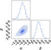 |
Fig. B.1. Posterior distributions of the parameters α and β in the core+envelope case. |
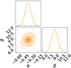 |
Fig. B.2. Posterior distributions of the parameters α and β in the fully mixed case. |
Appendix C: The mass-metallicity relation
Figure C.1 shows the mass-metallicity relations obtained when considering either a different planetary mass range or a smaller sample with more accurate measurements. In Sect. 4 we presented the mass-metallicity relation obtained for the core+envelope (CE) and fully mixed (FM) structures, using CMS19+HG23 and the full range of planetary masses (from 0.1 to 10 MJ). We found the following values for the parameters α and β of the power-law Zplanet/Zstar = β × M[MJ]α: α = −0.37 ± 0.07 and β = 8.61 ± 0.88 in the FM case and α = −0.57 ± 0.13 and β = 5.09 ± 0.95 in the CE case.
First we use a tighter range of planetary masses that correspond to the giant planet regime, with masses between 0.2 and 2 MJ (Helled 2023). For this range we now find: α = −0.379 ± 0.16 and β = 7.81 ± 1.28 in the FM case and α = −0.48 ± 0.24 and β = 4.72 ± 1.21 in the CE case. While the slope of the mass-metallicity relation has not changed in the FM case, it has decreased in the CE case. Overall, with both internal structures, the inferred planetary bulk metallicities are lower than those inferred when considering the full range of planetary masses.
Second, we derived the mass-metallicity relation for the larger mass range as presented in the main text, but considering only planets with a relative error in their observed radius smaller than 3%. 24 planets from our sample meet this criterion. This time, we find: α = −0.39 ± 0.11 and β = 7.15 ± 1.18 in the FM case and α = −0.60 ± 0.23 and β = 4.12 ± 1.24 in the CE case. For both internal structures, the slope of these relations remained similar. However, the inferred bulk metallicities are lower than those obtained when considering also planets with larger measurement uncertainties in the planetary radius (σR/R < 8%).
The analysis presented in this appendix demonstrates the importance of the chosen sample in inferring the mass-metallicity relation. As a result, caution should be taken when comparing relations inferred by different studies. In addition, it is also clear that having more planets with small measurement uncertainties is crucial for the investigation of trends in exoplanetary data.
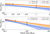 |
Fig. C.1. Top panel: Mass-metallicity relation considering different planetary mass ranges. Orange and blue lines show the best fit for the fully mixed (FM) and core+envelope (CE) cases when considering planets of masses between only 0.2 and 2 MJ. The shaded areas show the 1σ error contour. The relations previously obtained (see Sect. 4) when considering the full range of planetary masses (from 0.1 to 10 MJ) are shown with dotted lines. The metallicities of Jupiter and Saturn are shown in black. Bottom panel: Mass-metallicity relation considering different precision on observed radius. Orange and blue lines show the best fit for the fully mixed (FM) and core+envelope (CE) cases when only considering planets with relative uncertainties on radii which are less than 3%. The previously obtained relations, shown with dotted lines, include planets with an uncertainty on radius of up to 8%. |
All Tables
All Figures
|
Fig. 1. Radius vs. time for planets with masses of 0.3, 1, and 3 MJ (top, middle, and bottom panels, respectively). Left (right) panels correspond to models assuming a core+envelope (fully mixed) structure. Results with different H–He EOSs are shown with dashed and solid lines. The colours correspond to different assumed metallicities. The middle and bottom panels have similar limits on the y-axis, but not the top panels. |
| In the text | |
|
Fig. 2. Relative difference in density between the CMS19+HG23 (Chabrier et al. 2019; Howard & Guillot 2023) and SCvH95 (Saumon et al. 1995) EOSs. Blue regions on the T–P diagram indicate where CMS19+HG23 is denser than SCvH95, while red regions highlight less dense areas. The coloured solid and dashed lines show T–P profiles of some models (using CMS19+HG23) from Fig. 1, at 0.1 or 10 Gyr. The dotted square indicates the region of the ab initio presented by Militzer & Hubbard (2013). The CMS19+HG23 EOS is more accurate in this region. The hashed area corresponds to the region where hydrogen becomes solid (see e.g. Chabrier et al. 2019). |
| In the text | |
|
Fig. 3. Inferred heavy-element mass vs. planetary mass. Top panels: comparison of the results obtained with CMS19+HG23 and SCvH95, for both core+envelope and fully mixed structures. The circles represent the midpoint between the upper and lower bounds of the errorbars. Middle panels: absolute difference in heavy-element mass due to the H–He EOS update. Bottom panels: absolute difference in bulk metallicity. Empty circles correspond to planets for which CMS19+HG23 leads to a higher metallicity than SCvH95. The dotted black line shows the 1/Mp curve. |
| In the text | |
|
Fig. 4. Mass–metallicity relation with both interior structures, using the CMS19+HG23 EOS. Top panel: errorbars show the inferred range of bulk metallicity with the core+envelope (blue) or fully mixed (orange) structure, as in Fig. 3. Orange and blue lines show the best fit for both cases, while the shaded areas show the 1σ error contour. The metallicities of Jupiter and Saturn (Helled & Howard 2024) are shown in black. The solid and dashed grey lines show the best fits from Müller & Helled (2023) and Thorngren et al. (2016), respectively. The star metallicities were derived using the solar value from Asplund et al. (2021). Middle panel: absolute difference in metallicity due to either the H–He EOS (grey dots, taken from Fig. 3) or the interior structure (squares). Blue (orange) squares indicate planets where the core+envelope case gives lower (higher) metallicity than the fully mixed case. Bottom panel: absolute difference in metallicity. Pink dots show the sum of the H–He EOS and the interior structure effects. Black triangles show the range of metallicity inferred from observational uncertainties (radius and age). |
| In the text | |
|
Fig. B.1. Posterior distributions of the parameters α and β in the core+envelope case. |
| In the text | |
|
Fig. B.2. Posterior distributions of the parameters α and β in the fully mixed case. |
| In the text | |
|
Fig. C.1. Top panel: Mass-metallicity relation considering different planetary mass ranges. Orange and blue lines show the best fit for the fully mixed (FM) and core+envelope (CE) cases when considering planets of masses between only 0.2 and 2 MJ. The shaded areas show the 1σ error contour. The relations previously obtained (see Sect. 4) when considering the full range of planetary masses (from 0.1 to 10 MJ) are shown with dotted lines. The metallicities of Jupiter and Saturn are shown in black. Bottom panel: Mass-metallicity relation considering different precision on observed radius. Orange and blue lines show the best fit for the fully mixed (FM) and core+envelope (CE) cases when only considering planets with relative uncertainties on radii which are less than 3%. The previously obtained relations, shown with dotted lines, include planets with an uncertainty on radius of up to 8%. |
| In the text | |
Current usage metrics show cumulative count of Article Views (full-text article views including HTML views, PDF and ePub downloads, according to the available data) and Abstracts Views on Vision4Press platform.
Data correspond to usage on the plateform after 2015. The current usage metrics is available 48-96 hours after online publication and is updated daily on week days.
Initial download of the metrics may take a while.