© ESO 2022

1. Introduction

Fast radio bursts (FRBs) are transient radio signals with a duration of milliseconds (ms), flux of ∼0.1 − 1 Jy, and a large dispersion measure (DM; Cordes & Chatterjee 2019; Petroff et al. 2019; Zhang 2020; Xiao et al. 2021). The first recorded FRB, named the “Lorimer burst” (also known as FRB 010724), was discovered in 2007 (Lorimer et al. 2007) after this signal was first detected by the Parkes 64-m telescope in Australia on July 24, 2001. Recently, there have been two intriguing discoveries. One is that a period of 16.35 d (CHIME/FRB Collaboration 2020a) and a period of 157 d (Rajwade et al. 2020; Cruces et al. 2021) were found in FRB 180916 and FRB 121102, respectively. The other is that FRB 200428 was detected (Bochenek et al. 2020; CHIME/FRB Collaboration 2020b) and was related to a hard X-ray burst originating from SGR 1935+2154 in the Milky Way (Li et al. 2021a; Mereghetti et al. 2020; Ridnaia et al. 2021; Tavani et al. 2021). This suggests that at least a portion of FRBs are produced by magnetars. Some theoretical models based on magnetars have been proposed (Kulkarni et al. 2014; Lyubarsky 2014; Katz 2016; Murase et al. 2016; Beloborodov 2020; Metzger et al. 2019; Wang et al. 2020). Interestingly, the statistical properties of the repeating bursts are consistent with Galactic magnetar bursts (Wang & Yu 2017; Wadiasingh & Timokhin 2019; Cheng et al. 2020; Zhang et al. 2021; Wei et al. 2021; Sang & Lin 2022).

The first repeating FRB, FRB 121102 (Spitler et al. 2016), was found to be in an extreme magnetized environment (Michilli et al. 2018), which was revealed by the very high rotation measure (RM ∼ 10⁵ rad m⁻²). The RM decreases by ∼34% in 2.6 yr (Hilmarsson et al. 2021). The high and rapidly variable RM can be well understood in the magnetar nebula model (Margalit & Metzger 2018; Katz 2021a). An increase in the DM of FRB 121102 was found from long-term observations (Hessels et al. 2019; Josephy et al. 2019; Oostrum et al. 2020; Li et al. 2021b). The DM and RM evolution of FRB 121102 can be associated with the expanding magnetar wind nebula and shocked shell in a compact binary merger scenario (Zhao et al. 2021). However, such abnormal variations of DM and RM seem absent for other FRBs. The DM of FRB 180916 is almost constant (ΔDM < 0.1 pc cm⁻³, CHIME/FRB Collaboration 2020a; Nimmo et al. 2021; Pastor-Marazuela et al. 2021). Pleunis et al. (2021) found that the RM of FRB 180916 is very small (RM ≈ 115 rad m⁻²) and shows very small variations (ΔRM ∼ 2 − 3 rad m⁻²). The small and stable RM implies that the environmental magnetic field strength is much lower than that of FRB 121102. From the upper limits of X-ray and γ-ray emission, Tavani et al. (2020) gave constraints on the dissipation of magnetic energy of FRB 180916, which is inconsistent with the model involving strong magnetic field.

Using the simultaneous observations of FRB 180916 from the Apertif receiver (1220 MHz and 1520 MHz) on the Westerbork Synthesis Radio Telescope and the Low Frequency Array (LOFAR, 110 MHz and 190 MHz), Pastor-Marazuela et al. (2021) found that the active window of FRB 180916 is narrower and earlier at higher frequencies. The activity window at 150 MHz is narrower than those at 600 MHz and 1.4 GHz, and its peak activity is about 0.7 days earlier than that observed by CHIME/FRB in 600 MHz. The full width at half height of the activity of FRB 180916 observed by Apertif is 1.1 days, while that observed by CHIME/FRB is 2.7 days. Furthermore, the peak of the active period observed by LOFAR seems to arrive about 2 days later than that observed by CHIME/FRB, but their low number of detections prevents them from obtaining a better estimate of the active window.

The source of FRB 121102 is assumed to be a young magnetar with an age of ∼10 − 40 yr (Margalit & Metzger 2018). Marcote et al. (2020) speculated that the age of the progenitor of FRB 180916 is likely to be about 300 years based on the same RM decay model of FRB 121102. From the distance to the nearest young stellar clump, Tendulkar et al. (2021) inferred an age for the progenitor for FRB 180916 of between 800 kyr and 7 Myr, which seems to be inconsistent with the young active magnetars. But if the magnetar was born in the compact binary mergers, the observed spatial offset is also possible. In this work, we follow the young magnetar models and the age speculation from Marcote et al. (2020).

To explain the periodic activity, several types of models were proposed, including the collisions of pulsars and extra-galactic asteroid belts (Dai & Zhong 2020), the orbital models (Ioka & Zhang 2020; Lyutikov et al. 2020; Wada et al. 2021; Li et al. 2021c), the precession models (Levin et al. 2020; Sob’yanin 2020; Tong et al. 2020; Yang & Zou 2020; Zanazzi & Lai 2020; Chen et al. 2021) and the rotation period model (Beniamini et al. 2020; Xu et al. 2021). Recently, Katz (2021b) tested some types of period models based on observations by Pastor-Marazuela et al. (2021) and Pleunis et al. (2021). Little work has been carried out to evaluate these period models, especially those based on the latest observations, which are discussed below.

In this work, we provide constraints on these models for FRB 180916 using recent observations (Marcote et al. 2020; Pastor-Marazuela et al. 2021; Pleunis et al. 2021; Tavani et al. 2020). In addition, to explain the 16-day period, the predictions of these models should also be consistent with the stable DM and RM, the frequency-dependent active window, the weak internal magnetic field, and the age of about 300 years. Because of the limitations of the observations, we only tested the orbital models, precession models, and rotational models. We find that the geodetic precession model is the most likely model for FRB 180916.

The rest of this paper is organized as follows. Section 2 shows the observations used in this paper. In Sect. 3, we constrain several types of period models using these recent observations. Finally, we provide a discussion of our results and a summary in Sect. 4.

2. Recent observational results

Four observations are used in this paper to constrain periodic models. The first observation is that Pastor-Marazuela et al. (2021), using simultaneous observations of FRB 180916 from the Apertif and LOFAR, found that the active window of FRB 180916 is narrower and earlier at a higher frequency. In addition, the dispersion measure (DM) is constant in the observations at these frequencies, and the maximum signal-to-noise DM is 349.00 pc cm⁻³ in the LOFAR observations. Furthermore, Pleunis et al. (2021) found that the value of RM of FRB 180916 is very small, RM ≈ 115 rad m⁻².

The second observation is based on the observation of FRB 180916 (Pastor-Marazuela et al. 2021; Pleunis et al. 2021); Katz (2021b) proposed a limitation on the variation of angular velocity $\dot{\mathrm{\Omega }}$:

$$\begin{array}{c}\hfill |\dot{\mathrm{\Omega }}|=\frac{8|\mathrm{\Delta }\varphi |}{T^2}\lesssim 5\times {10}^{-16}{\mathrm{s}}^{-2},\end{array}$$(1)

where Δϕ is the phase deviation from the exact periodic endpoint in a period fitted by the midpoint of the data, T = 49 P ≈ 7 × 10⁷ s is the observation duration, and P is the observation period. It is assumed that the angular velocity Ω is fitted to the data from the whole data interval T and Katz (2021b) proposed |Δϕ|≲0.05 cycle ≈ 0.3 radian which is estimated from the observation of Pastor-Marazuela et al. (2021) and Pleunis et al. (2021). Also, Katz (2021b) mentions that Eq. (1) will rapidly become more stringent as T increases, or that a significant non-zero rate of angular velocity change $\dot{\mathrm{\Omega }}$ will be observed.

The third observation is that based on the X-ray and γ-ray observation results of FRB 180916 obtained by Astro-Rivelatore Gamma a Immagini Leggero (AGILE) and Swift: Tavani et al. (2020) derived the most stringent constraints so far which are applicable to magnetar-type neutron stars:

$$\begin{array}{c}\hfill R_{\mathrm{m},6}^3{B}_{\mathrm{int},16}^2{\tau }_{\mathrm{d},8}^{-1}\lesssim 1,\end{array}$$(2)

where R_m is the magnetospheric radius of the magnetar, B_int is the internal magnetic field intensity, and τ_d is the ambipolar diffusion timescale of the internal magnetic field. In addition, limited by the observation time, the magnetic dissipation timescale τ_d is ∼10³ − 10⁵ s. Therefore, if we set R_m to be 10⁶ cm, the value of B_int should be ∼10^13.5 − 10^14.5 G, as shown in Fig. 1.

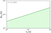Fig. 1. Constraint on the internal magnetic field Bint according to Eq. (1). The green line shows the condition of Rm = 106 cm. The colored area represents the allowed range of the internal magnetic field when the value of τd is from 103 s to 105 s.

The fourth observation is that Marcote et al. (2020) estimated the age of the progenitor of FRB 180916 to be about 300 years. Therefore, assuming that the progenitor of FRB 180916 is a magnetar and combining the relation between the age t and the rotation period P_rot of magnetar (Levin et al. 2020):

$$\begin{array}{c}\hfill t\approx 7.5\mathrm{yr}{P}_{\mathrm{rot},0}^2{B}_{\mathrm{dip},15}^{-2},\end{array}$$(3)

we can get the rotation period P_rot = 2 s for the progenitor.

3. Constraints on periodic models

In this section, we use the observations described in Sect. 2 to constrain the periodic models for FRB 180916. We mainly limit ourselves to three types of periodic model:

1. Orbital model: In a binary system, FRBs are generated by a neutron star. This radio wave might therefore be obscured by or interact with the wind of the companion star, which could cause the periodicity (Ioka & Zhang 2020; Lyutikov et al. 2020).

2. Precession models: The precession might be caused by the free precession of a magnetically twisted nonspherical neutron star (Levin et al. 2020; Zanazzi & Lai 2020) or the forced precession which might be caused by the anomalous electromagnetic moment (Sob’yanin 2020) or the fall-back disk (Tong et al. 2020), or the orbital induced spin precession of the neutron star in a binary system (Yang & Zou 2020). For convenience, we refer to these as the free precession model, the radiation-driven precession model, the fall-back disk precession model, and the geodetic precession model, respectively.

3. Rotation model: the observational period is regarded as the rotation period of a neutron star (Beniamini et al. 2020; Xu et al. 2021).

Additionally, in the following sections, we use the sign A_x = A/10^x in the cgs unit. Unless specifying otherwise, in the following calculations we regard the mass of the neutron star to be M_ns = 1.4 M_⊙ and the radius of the neutron star to be R_ns = 10⁶ cm.

3.1. Constraints on the orbital period model

According to the first observation introduced in Sect. 2, the DM should be a constant, which is consistent with the orbital period model. In addition, according to this observation, the RM is very small (∼100 rad m⁻²) and the active window should be narrower at higher frequencies. However, for the orbital period model, the predicted RM is very large (∼10³ rad m⁻²) and the active window will be wider on a higher frequency. Therefore, this model cannot explain the periodicity of FRB 180916. Wada et al. (2021) proposed two possible scenarios to explain this phenomenon, but these two scenarios need extremely strict conditions.

3.2. Constraints on the precession model

In this section, we mainly use the second and third observations to constrain these period models, except the orbital period model.

3.2.1. Constraints on the free precession model

For the free precession model, the derivation of the period of the precession Ṗ_pre is

$$\begin{array}{c}\hfill {\dot{P}}_{\mathrm{pre}}=\frac{P_{\mathrm{pre}}}{2t},\end{array}$$(4)

where P_pre is the precession period and t is the age of the neutron star. It should be noted that in Levin et al. (2020), the actual age t of the neutron star is used to calculate the precession period P_pre, but Katz (2021b) proposed that the spin-down timescale t_sd may be more appropriate because the neutron star may be born when its spin period and precession period are close to the current value. The t_sd is derived as

$$\begin{array}{c}\hfill t_{\mathrm{sd}}=\frac{12c^3{M}_{\mathrm{ns}}}{5B_{\mathrm{dip}}^2{R}_{\mathrm{ns}}^4{\mathrm{\Omega }}_{\mathrm{rot}}^2}\approx 144.6\mathrm{yr}{B}_{\mathrm{dip},15}^{-2}{R}_{\mathrm{ns},6}^{-4}\left(\frac{M_{\mathrm{ns}}}{1.4M_{\odot }}\right)P_{\mathrm{rot},0}^2,\end{array}$$(5)

where B_dip is the dipole field and Ω_rot = 2π/P_rot is the spin angular frequency.

Combining this latter equation with Eq. (4), we can obtain the change rate of precession angular velocity:

$$\begin{array}{c}\hfill {\dot{\mathrm{\Omega }}}_{\mathrm{pre}}=-\frac{{\mathrm{\Omega }}_{\mathrm{pre}}}{2t}·\end{array}$$(6)

Combining Eq. (1) with |Δϕ|≲0.3 radian and T ≈ 7 × 10⁷ s, we can rewrite the above equation as

$$\begin{array}{c}\hfill t=\frac{\pi T^2}{8P_{\mathrm{pre}}|\mathrm{\Delta }\varphi |}\gtrsim 150\mathrm{yr}.\end{array}$$(7)

In this way, we can obtain a lower limit on the age of the neutron star which is consistent with the 300-year age of the magnetar of FRB 180916 speculated by Marcote et al. (2020). This lower limit might increase rapidly as the observation time increases because it is highly dependent on T. In this way, this model can be thoroughly tested in future.

Also, Zanazzi & Lai (2020) gave the relationship between rotation period P_rot and precession period P_pre of the magnetar (also see in Levin et al. 2020):

$$\begin{array}{c}\hfill P_{\mathrm{pre}}=\frac{P_{\mathrm{rot}}}{ϵ\cos \theta },\end{array}$$(8)

where ϵ is the ellipticity and θ is the angle between the rotation angular velocity vector Ω and the principle axis with the greatest moment of inertia, which we call the z-axis in the following. Levin et al. (2020) set the value of θ to 0. Zanazzi & Lai (2020) considered five factors that may contribute to the ellipticity ϵ but finally decided that just four of them are possible.

If we use the spin-down age t_sd of the neutron star to replace t, we can get the dipole field B_dip by combining Eq. (7) with Eqs. (8) and (5):

$$\begin{array}{c}\hfill B_{\mathrm{dip}}=ϵ\cos \theta \sqrt{\frac{3c^3{M}_{\mathrm{ns}}{P}_{\mathrm{pre}}^3|{\dot{\mathrm{\Omega }}}_{\mathrm{pre}}|}{5{\pi }^3{R}_{\mathrm{ns}}^4}}=ϵ\cos \sqrt{\frac{24c^3{M}_{\mathrm{ns}}{P}_{\mathrm{pre}}^3|\mathrm{\Delta }\varphi |}{5{\pi }^3{R}_{\mathrm{ns}}^4{T}^2}}·\end{array}$$(9)

Firstly, for the ellipticity caused by the internal magnetic field, ϵ = ϵ_mag, the internal magnetic field B_int gives

$$\begin{array}{c}\hfill {ϵ}_{\mathrm{mag}}=\beta \frac{R_{\mathrm{ns}}^4{B}_{\mathrm{int}}^2}{G_0{M}_{\mathrm{ns}}^2}\approx k\times {10}^{-4}{B}_{\mathrm{int},16}^2{R}_{\mathrm{ns},6}^4{\left(\frac{M_{\mathrm{ns}}}{1.4M_{\odot }}\right)}^{-2},\end{array}$$(10)

where G₀ is the gravitational constant, and R_ns and M_ns are the radius and the mass of the magnetar, which we set to be the typical values of the neutron star. β and k are the numerical coefficients which should satisfy |β|≤1 and k ≤ 1, and Levin et al. (2020) thought that k ≪ 1 in this condition. Using the magnetic field value of B_dip ∼ 0.1 B_int in the shock maser model of FRB, we can derive the limitation of B_int with Eq. (9):

$$\begin{array}{c}\hfill \begin{array}{cc}& B_{\mathrm{int}}=\frac{G_{0}T}{10k{R}_{\mathrm{ns}}^2\cos \theta }\sqrt{\frac{5{\pi }^3{M}_{\mathrm{ns}}^3}{24c^3{P}_{\mathrm{pre}}^3|\mathrm{\Delta }\varphi |}}\hfill \\ \hfill & B_{\mathrm{int}}\gtrsim 3.7\times {10}^{13}\mathrm{G}{k}^{-1}{(\cos \theta )}^{-1},\hfill \end{array}\end{array}$$(11)

where k ≪ 1. This equation gives a lower limit on the internal field. In this equation, if k = 0.12 is assumed and cos θ takes the maximum value which is 1, we can obtain the limit of the internal magnetic field, that is ≳3 × 10¹⁴ G, which is consistent with the third observation in Sect. 2 (i.e., that the magnitude of B_int should be ∼10^13.5 − 10^14.5 G). In addition to adjusting the value of k, B_dip ∼ 0.1 B_int is also uncertain, and the predicted values of this model can be adjusted to conform to the observations, as shown in Fig. 2.

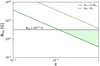Fig. 2. Relation between the internal magnetic field Bint and the numerical coefficient k is drawn according to Eq. (9). The black horizontal line represents the maximum value of the internal magnetic field limited by Eq. (2) when the magnetosphere radius Rm = 106 cm. In addition, the green lines show the relationship between Bint and k drawn from Eq. (9). We show two different conditions, Bdip ∼ 0.1 Bint and Bdip ∼ Bint. The colored area shows the allowable region.

It is important to note that Eq. (7) in Katz (2021b) contains a typo, where the exponent of k should be 1 instead of 2. The correct equation should be

$$\begin{array}{c}\hfill B\sim \frac{{10}^{36}{\mathrm{G}}^2}{k}\sqrt{\frac{{\sin }^2\theta R^6{\pi }^3{T}^2}{6I{c}^3{P}_{\mathrm{pre}}^3\mathrm{\Delta }\varphi }}=5\times {10}^{14}\mathrm{G}\frac{\sin \theta }{k}\sqrt{\frac{0.3}{\mathrm{\Delta }\varphi }}\frac{T}{1\mathrm{yr}}·\end{array}$$(12)

Also, Katz (2021b) used the approximation of B_int ∼ B_dip, and in this paper we use B_dip ∼ 0.1 B_int. Furthermore, we also use other different relationships to get the limit of the magnetic field. In this way, the condition that the limitation in this paper is different from that of Katz (2021b) can be understood. And these two limitations can be confirmed by each other.

Secondly, for the ellipticity caused by the near-region dipole field associated with neutron stars, its ellipticity is

$$\begin{array}{c}\hfill {ϵ}_{\mathrm{dip}}=\frac{3B_{\mathrm{dip}}^2{R}_{\mathrm{ns}}^5}{20I{c}^2}\approx 1.5\times {10}^{-7}{B}_{\mathrm{dip},15}^2{R}_{\mathrm{ns},6}^3{\left(\frac{M_{\mathrm{ns}}}{1.4M_{\odot }}\right)}^{-1},\end{array}$$(13)

where $I=\frac{2}{5}{M}_{\mathrm{ns}}{R}_{\mathrm{ns}}^2$ is the rotational inertia of the magnetar. We can obtain the limitation of this dipole field with Eqs. (9) and (13):

$$\begin{array}{c}\hfill B_{\mathrm{dip}}=\frac{4T}{3R_{\mathrm{ns}}\cos \theta }\sqrt{\frac{5{\pi }^{3}c{M}_{\mathrm{ns}}}{6P_{\mathrm{pre}}^3|\mathrm{\Delta }\varphi |}}\gtrsim 4.7\times {10}^{15}\mathrm{G}{(\cos \theta )}^{-1}.\end{array}$$(14)

This equation gives a lower limit of the dipole magnetic field, and even if the (cosθ)⁻¹ takes the minimum value of 1, it will exceed the magnetic field range of the observed limit.

Thirdly, for the ellipticity caused by the two components B_∥ and B_δ of the quadrupole magnetic field associated with the neutron star, ϵ ∼ ϵ_∥ and ϵ ∼ ϵ_δ. According to Zanazzi & Lai (2020), we have

$$\begin{array}{c}\hfill \begin{array}{cc}& {ϵ}_{\Vert }=\frac{4}{105}{\left(\frac{B_{\Vert }}{B_{\mathrm{dip}}}\right)}^2{ϵ}_{\mathrm{dip}}\approx 5.7\times {10}^{-7}{B}_{\Vert ,16}^2{R}_{\mathrm{ns},6}^3{\left(\frac{M_{\mathrm{ns}}}{1.4M_{\odot }}\right)}^{-1},\hfill \\ \hfill & {ϵ}_{\delta }=\frac{16}{945}{\left(\frac{B_{\delta }}{B_{\mathrm{dip}}}\right)}^2{ϵ}_{\mathrm{dip}}\approx 2.5\times {10}^{-7}{B}_{\delta ,16}^2{R}_{\mathrm{ns},6}^3{\left(\frac{M_{\mathrm{ns}}}{1.4M_{\odot }}\right)}^{-1}.\hfill \end{array}\end{array}$$(15)

Combined with Eqs. (9) and (15), the limitation of these two components is

$$\begin{array}{c}\hfill \begin{array}{cc}& B_{\Vert }=\frac{35T}{R_{\mathrm{ns}}\cos \theta }\sqrt{\frac{5{\pi }^{3}c{M}_{\mathrm{ns}}}{6P_{\mathrm{pre}}^3|\mathrm{\Delta }\varphi |}}\gtrsim 1.2\times {10}^{17}\mathrm{G}{(\cos \theta )}^{-1},\hfill \\ \hfill & B_{\delta }=\frac{315T}{2R_{\mathrm{ns}}\cos \theta }\sqrt{\frac{5{\pi }^{3}c{M}_{\mathrm{ns}}}{24P_{\mathrm{pre}}^3|\mathrm{\Delta }\varphi |}}\gtrsim 2.8\times {10}^{17}\mathrm{G}{(\cos \theta )}^{-1}.\hfill \end{array}\end{array}$$(16)

Even if the (cosθ)⁻¹ takes the minimum value of 1, it also far exceeds the magnetic field range of the observation limit.

In summary, the free precession model with the ellipticity caused by the internal magnetic field can be adjusted to meet the observation by changing the values of the parameters, and the other two do not fit the observation.

3.2.2. Constraints on the radiation-driven precession model

For the radiation-driven precession model, if the magnetic field of the neutron star is represented by the magnetic field of the magnetic dipole, the neutron star is a dipole that is rotating with an angle θ for the distant observer. The change rate of radiation energy is

$$\begin{array}{c}\hfill {\dot{E}}_{\mathrm{rot}}=\frac{2{\mu }^2{\mathrm{\Omega }}_{\mathrm{rot}}^4{\sin }^2\theta }{3c^3},\end{array}$$(17)

where $\mu =\frac{1}{2}{B}_{\mathrm{dip}}{R}^3$ is the magnetic dipole moment. If we ignore the change of the moment of inertia, the change rate of radiation energy could be

$$\begin{array}{c}\hfill {\dot{E}}_{\mathrm{rot}}=\frac{\mathrm{d}(\frac{1}{2}I{\mathrm{\Omega }}_{\mathrm{rot}}^2)}{\mathrm{d}t}=I{\mathrm{\Omega }}_{\mathrm{rot}}{\dot{\mathrm{\Omega }}}_{\mathrm{rot}}.\end{array}$$(18)

We can then obtain the equation for slowing down the rotation of a neutron star (Ghosh 2007):

$$\begin{array}{c}\hfill {\dot{P}}_{\mathrm{rot}}=\frac{2}{3}{(2\pi )}^2\frac{{\mu }^2{\sin }^2\theta }{I{c}^3{P}_{\mathrm{rot}}}·\end{array}$$(19)

Sob’yanin (2020) gave the equation of the internal magnetic field of a precession neutron star:

$$\begin{array}{c}\hfill \begin{array}{cc}\hfill B_{\mathrm{int}}& =c\sqrt{\frac{15I}{2R_{\mathrm{ns}}^5\cos {\theta }_m}\frac{P_{\mathrm{rot}}}{P_{\mathrm{pre}}}\frac{1}{1+\lambda R_{\mathrm{ns}}/R_{\mathrm{g}}}}\hfill \\ \hfill & \approx 7.45\times {10}^{17}\mathrm{G}\sqrt{\frac{P_{\mathrm{rot}}}{P_{\mathrm{pre}}}},\hfill \end{array}\end{array}$$(20)

where θ_m is magnetic inclination, which is the angle between the rotation axis and the magnetic axis. In the second line of this equation, we use the typical value of the neutron star, and we set cosθ_m = 1 and λ = 3, which corresponds to taking β = 1 in ϵ_mag.

Combining this equation with Eq. (19), the change rate of the precession angular velocity is

$$\begin{array}{c}\hfill \begin{array}{cc}\hfill {\dot{\mathrm{\Omega }}}_{\mathrm{pre}}& =-\frac{30{\pi }^{3}c{G}_0^2{M}_{\mathrm{ns}}^3{B}_{\mathrm{dip}}^2{\sin }^2\theta }{R_{\mathrm{ns}}^2{(G_0{M}_{\mathrm{ns}}+\lambda R_{\mathrm{ns}}{c}^2)}^2{B}_{\mathrm{int}}^4{P}_{\mathrm{pre}}^3{\cos }^2{\theta }_{\mathrm{m}}}\hfill \\ \hfill & =(-1.2\times {10}^{-14}{\mathrm{s}}^{-2}{\mathrm{G}}^2)\frac{B_{\mathrm{dip}}^2{\sin }^2\theta }{B_{\mathrm{int}}^4{\cos }^2{\theta }_{\mathrm{m}}}·\hfill \end{array}\end{array}$$(21)

It can be seen that over time, the precession angular velocity of the neutron star will decrease, and the observation period predicted by this model will increase. Combining this equation with Eq. (1) and B_dip ∼ 0.1 B_int, the lower limitation on B_int is

$$\begin{array}{c}\hfill \begin{array}{cc}\hfill B_{\mathrm{int}}=& (1.1\times {10}^6{\mathrm{s}}^{-1}\mathrm{G})\frac{T|\sin \theta |}{|\cos {\theta }_{\mathrm{m}}|\sqrt{8|\mathrm{\Delta }\varphi |}}\hfill \\ \hfill & \gtrsim 4.9\times {10}^{13}\mathrm{G}\frac{|\sin \theta |}{|\cos {\theta }_{\mathrm{m}}|}\sim 4.9\times {10}^{13}\mathrm{G}.\hfill \end{array}\end{array}$$(22)

In the second line of the above equation, we set θ = θ_m = π/4. It is seen that if we set θ = θ_m, only θ ∉ [81.2° +kπ,  98.8° +kπ], (k ∈ ℤ) can meet the requirements of the observed magnetic field (B_int ≲ 10^14.5 G), as shown in Fig. 3.

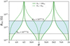Fig. 3. Relation between the internal magnetic field Bint and the angle θ is drawn according to Eq. (22). We set θ = θm which means the magnetic axis of the neutron star is aligned in the direction of the dipole axis. The black horizontal lines represent the maximum value of the internal magnetic field limited by Eq. (2). We show two conditions, which are Bint = 1014.5 G and Bint = 1013.5 G. Also, the green lines show the relationship between Bint and θ drawn from Eq. (22). Two different conditions are shown, Bint ∼ 10 Bdip and Bint ∼ Bdip. The colored areas show the allowable region.

It should be noted that Eq. (10) in Katz (2021b) also contains a typo, where the exponent of P_pre should be 3 instead of 1 and the whole equation is missing a minus sign. The correct equation should be

$$\begin{array}{c}\hfill {\dot{\mathrm{\Omega }}}_{\mathrm{pre}}=-\frac{2}{3}{(2\pi )}^3\frac{R^6{\sin }^2\theta }{I{c}^3{P}_{\mathrm{pre}}^3}\frac{{(7.45\times {10}^{17}\mathrm{G})}^4}{{(2B)}^2}·\end{array}$$(23)

In addition, this equation of Katz (2021b) was derived using the approximate formula in the radiation-driven model, and it is more accurate to apply Eq. (22) in this paper.

3.2.3. Constraints on the geodetic precession model

For the geodetic precession model, a neuron star with a mass of M₁ and a companion with a mass of M₂ = qM₁ form a compact binary system. It is assumed that the two stars both orbit around a circle with the same angular velocity in a binary system.

Yang & Zou (2020) gave the equation of the precession period of a neutron star:

$$\begin{array}{c}\hfill P_{\mathrm{pre}}=\frac{1+q}{q(4+3q)}\frac{4\pi c^2}{G_0{M}_1}(1-e^2)a^{5/2},\end{array}$$(24)

where e is the orbital eccentricity and a is the distance between the two stars.

Neglecting the mass loss and combined with Eq. (24), the change rate of the precession angular velocity is

$$\begin{array}{c}\hfill {\dot{\mathrm{\Omega }}}_{\mathrm{pre}}=32\frac{2^{21/5}{\pi }^{13/5}{(1+q)}^{9/5}}{q^{3/5}{(4+3q)}^{8/5}}\frac{{(G_0{M}_1)}^{3/5}}{c^{9/5}}{P}_{\mathrm{pre}}^{-13/5}.\end{array}$$(25)

It can be seen that the observation period of the neutron star predicted by this model will decrease over time. We can obtain the relationship between q and M₁ using Eq. (1) and the 16.3-day observation period of FRB 180916, as shown in Fig. 4. We find that, when q = 1, the mass of the neutron star is required to be less than 10 M_⊙, which satisfies the upper limit on the mass of the neutron star; when M₁ = 1.4 M_⊙, q ≳ 0.1 is required, which is also consistent with the mass of the compact companion star.

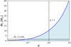Fig. 4. Relationship between the mass of the neutron star M1 and q drawn according to Eq. (25), as shown in blue line. The black horizontal solid line represents M1 = 1.4 M⊙ and the black vertical solid line shows q = 1. The blue area of this plot shows the area that matches the observation.

3.2.4. Constraints on the fall-back disk precession model

For the fall-back disk precession model with the eccentricity due to the strong magnetic field, Tong et al. (2020) gave its precession angular velocity as

$$\begin{array}{c}\hfill {\mathrm{\Omega }}_{\mathrm{pre}}=\frac{9ϵ}{4}\frac{M_{\theta }}{M_{\mathrm{ns}}{\kappa }^3}{\mathrm{\Omega }}_{\mathrm{rot}}.\end{array}$$(26)

In this equation, we set M_θ = M₀cosθ_fb (M₀ is the total mass of the fall-back disk and θ_fb is the angle between the axis of rotation of the neutron star and the normal direction of the plane of the fall-back disk), and we set R = κR_co (R is the distance between the neutron star and the fall-back disk, $R_{\text{co}}={(G_0{M}_{\text{ns}}/{\mathrm{\Omega }}_{\text{rot}}^2)}^{1/3}$ is the corotation radius, and R is the order of R_co). In addition, Tong et al. (2020) thought the value of M_θ is approximately 10⁻⁶ − 10⁻¹ M_⊙, and Qiao et al. (2003) assumed κ is from 1 (or smaller) to the value of 2 ∼ 3 when θ is varied within 0 ∼ 90°. We then take the derivative of this equation, and we let Ṁ_θ = 0, obtaining

$$\begin{array}{c}\hfill {\dot{\mathrm{\Omega }}}_{\mathrm{pre}}=\frac{9ϵ}{4}\frac{M_{\theta }}{M_{\mathrm{ns}}{\kappa }^3}{\dot{\mathrm{\Omega }}}_{\mathrm{rot}}.\end{array}$$(27)

Assuming that the spin-down of neutron stars is controlled by the magnetic dipole moment, the distance between the neutron star and the fall-back disk remains the same, and B_dip ∼ 0.1 B_int, we can eliminate Ω_rot and ${\dot{\mathrm{\Omega }}}_{\mathrm{rot}}$ in Eq. (27) by combining with Eq. (19). We then can obtain the rate of precession angular velocity change:

$$\begin{array}{c}\hfill {\dot{\mathrm{\Omega }}}_{\mathrm{pre}}=-\frac{640{\pi }^3{\mu }^2{\sin }^2\theta M_{\mathrm{ns}}{\kappa }^6}{243c^3{ϵ}^2{R}_{\mathrm{ns}}^2{P}_{\mathrm{pre}}^3{M}_{\theta }^2}·\end{array}$$(28)

For $\mu =\frac{1}{2}{B}_{\mathrm{dip}}{R}_{\mathrm{ns}}^3$ and $ϵ={10}^{-4}{B}_{\text{int},\text{16}}^2$, we can obtain the internal magnetic field by combining with Eq. (1):

$$\begin{array}{c}\hfill \begin{array}{cc}\hfill B_{\mathrm{int}}=& (\frac{4}{9}\times {10}^{35}{\mathrm{G}}^2)\sqrt{\frac{10{\pi }^3{\kappa }^6{R}_{\mathrm{ns}}^4{M}_{\mathrm{ns}}{\sin }^2\theta }{3c^3{M}_{\theta }^2{P}_{\mathrm{pre}}^3|\dot{\mathrm{\Omega }}|}}\hfill \\ \hfill & \gtrsim 6.2\times {10}^{14}\mathrm{G}|\sin \theta |\frac{0.1M_{\odot }}{M_{\theta }}·\hfill \end{array}\end{array}$$(29)

In the second line of this equation, we set κ = 1 and P_pre = 16.3 d. In addition, we take the maximum mass of the fall-back disk as 0.1 M_⊙. If the magnetic field strength is required to meet observations, the angle between the dipole axis and the rotation axis needs to satisfy θ ∈ ( − 30.6° +kπ, 30.6° +kπ),k ∈ ℤ.

For the eccentricity due to the rotation, according to Katz (2021b), for the change rate of the precession angular velocity, we can make the qualitative prediction which is ${\dot{\mathrm{\Omega }}}_{\mathrm{pre}}\sim -{\mathrm{\Omega }}_{\mathrm{pre}}/t_{\mathrm{diss}}$, where t_diss is the dissipation time of the fall-back disk. According to Eq. (1), the lower limit on the dissipation time of the fall-back disk is 9.1 × 10⁹ s. However, there is no clear calculation for the dissipation time of the disk. In the future, this model might be tested using this limitation.

3.2.5. Constraints on the rotation model

In this section, we consider the model where the spin-down is due to the fallback of the long-time accretion disk. Beniamini et al. (2020) gave the final rotation period of the magnetar at the magnetic field decay time ${\tau }_{\mathrm{B}}=880\mathrm{yr}{B}_{\mathrm{int},16}^{-6/5}$:

$$\begin{array}{c}\hfill P_{\mathrm{rot}}=P_{\mathrm{c}}{\left(\frac{{\tau }_{\mathrm{B}}}{t_{\mathrm{fb}}}\right)}^{3\zeta /7},\end{array}$$(30)

where $P_{\mathrm{c}}=1.5\mathrm{ms}{B}_{\mathrm{dip},15}^{6/7}{\dot{M}}_{\mathrm{i},-2}^{-3/7}{(\frac{M_{\mathrm{ns}}}{1.4M_{\odot }})}^{-5/7}$ is the rotation period of the magnetar in the steady state, M_i is the initial mass of the accretion disk, and t_fb is the initial fall-back time.

By combining with Eq. (30), setting the initial mass of the fall-back disk to 10⁻² M_ns, and using ζ = 2, t_fb = 10 s, and B_int ∼ 10 B_dip = 10^14.5 G, we can obtain the change rate of angular velocity with the period of 16.3 d:

$$\begin{array}{c}\hfill |\dot{\mathrm{\Omega }}|\approx 2.9\times {10}^{-7}{\mathrm{s}}^{-2}{B}_{\mathrm{int},14.5}^{-6/35}.\end{array}$$(31)

We can then obtain the limit on the systemic moment $N=I\dot{\mathrm{\Omega }}$:

$$\begin{array}{c}\hfill N\lesssim \frac{8\mathrm{\Delta }\varphi }{T^2}I\sim 4.9\times {10}^{29}\mathrm{dyne}\mathrm{cm}.\end{array}$$(32)

If this is interpreted as the accretion of a neutron star of mass 1.4 M_⊙ and radius 10⁶ cm, then considering the most simplified case, the corresponding limit on the accretion rate Ṁ introduced by $N=\frac{\mathrm{d}(I\mathrm{\Omega })}{\mathrm{d}t}=\frac{3}{5}\sqrt{G_0{R}_{\mathrm{ns}}{M}_{\mathrm{ns}}}\dot{M}$ is ≲5.1 × 10¹³ g s⁻¹ ≈ 9.6 × 10⁻¹³ M_⊙ yr⁻¹, which is much smaller than the known accretion rate of massive X-ray binaries (NS-OB stars). This model is therefore not representative.

3.3. Testing models using the phase shift

For the orbital period model, its predicted observation period should be constant. Therefore, regardless of how large T is, |Δϕ| is always zero, as shown by the red solid line in Fig. 5.

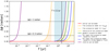Fig. 5. Relation between the phase shift Δϕ and the observation duration T for FRB 180916 by combining Eq. (1) with Eq. (2) in different models. The orange and yellow lines represent an upper limit and the blue dashed line represents a lower limit. The colored area can fit the observation. The solid vertical line shows T = 2.2 yr. The rotation period model does not fit the observation of |Δϕ|≲0.3 radian. The two dashed parallel lines mean Δϕ = 1 radian and Δϕ = 0.3 radian, respectively. These models can be tested by verifying whether or not there will be a detectable phase shift within a longer observation duration.

For the free precession model, we can rewrite Eq. (9) as

$$\begin{array}{c}\hfill {\dot{\mathrm{\Omega }}}_{\mathrm{pre}}=-\frac{5{\pi }^3{B}_{\mathrm{dip}}^2{R}_{\mathrm{ns}}^4}{3c^3{M}_{\mathrm{ns}}{P}_{\mathrm{pre}}^3{ϵ}^2{\cos }^2\theta }·\end{array}$$(33)

If the ellipticity is caused by the internal magnetic field, that is ϵ ∼ ϵ_mag, and B_int = 10 B_dip ≲ 10^14.5 G is assumed, we obtain

$$\begin{array}{c}\hfill {\dot{\mathrm{\Omega }}}_{\mathrm{pre}}=-\frac{{\pi }^3{G}_0^2{M}_{\mathrm{ns}}^3}{60c^3{k}^2{R}_{\mathrm{ns}}^4{B}_{\mathrm{int}}^2{P}_{\mathrm{pre}}^3{\cos }^2\theta }\gtrsim -6.7\times {10}^{-18}{\mathrm{s}}^{-2}{k}^{-2}{(\cos \theta )}^{-2},\end{array}$$(34)

where we set k ≈ 0.12 and θ = 0. We therefore have $|{\dot{\mathrm{\Omega }}}_{\mathrm{pre}}|\lesssim 6.7\times {10}^{-16}$ s⁻². Subsequently, when the phase shift |Δϕ| = 1 radian, the lower limit on the desired duration is approximately 1.3 × 10⁸ s ∼ 4.2 yr, which can be used to test this model, shown as the orange solid line in Fig. 5. If the ellipticity is caused by the dipole field, i.e., ϵ ∼ ϵ_dip, we have

$$\begin{array}{c}\hfill {\dot{\mathrm{\Omega }}}_{\mathrm{pre}}=-\frac{320{\pi }^{3}c{M}_{\mathrm{ns}}}{27R_{\mathrm{ns}}^2{B}_{\mathrm{dip}}^2{\cos }^2\theta P_{\mathrm{pre}}^3}\gtrsim -3.3\times {10}^{-13}{\mathrm{s}}^{-2}.\end{array}$$(35)

Therefore, we have $|{\dot{\mathrm{\Omega }}}_{\mathrm{pre}}|\lesssim 3.3\times {10}^{-13}$ s⁻², and if we set |Δϕ| = 1 radian, the lower limit on T approximately is 4.9 × 10⁶ s ∼ 0.4 yr, as shown by the orange dashed line in Fig. 5. But no such phase shift has been observed with current observation time (T ≈ 2.2 yr).

For the radiation-driven precession model, assuming B_int = 10 B_dip ≲ 10^14.5 G and combining with Eq. (22), the limit on the change rate of precession angular velocity is

$$\begin{array}{c}\hfill {\dot{\mathrm{\Omega }}}_{\mathrm{pre}}\gtrsim -1.2\times {10}^{-17}{\mathrm{s}}^{-2}.\end{array}$$(36)

We therefore have $|{\dot{\mathrm{\Omega }}}_{\mathrm{pre}}|\lesssim 1.2\times {10}^{-17}$ s⁻², and when |Δϕ| = 1 radian, the lower limit on T is approximately 8.2 × 10⁸ s ∼ 25.9 yr, as shown by the solid yellow line in Fig. 5.

For the geodetic precession model, combining with Eq. (25) and assuming q = 1 and M₁ = 1.4 M_⊙, the change rate of angular velocity is

$$\begin{array}{c}\hfill {\dot{\mathrm{\Omega }}}_{\mathrm{pre}}=1.5\times {10}^{-16}{\mathrm{s}}^{-2}.\end{array}$$(37)

For |Δϕ| = 1 radian, we can get T ≈ 2.3 × 10⁸ s ∼ 7 yr, as shown by the green solid line in Fig. 5.

For the fall-back disk precession model, if the eccentricity is caused by the rotation of the neutron star, combining with ${\dot{\mathrm{\Omega }}}_{\mathrm{pre}}\sim -\mathrm{\Omega }/t_{\mathrm{diss}}$ and assuming that t_diss ∼ 10¹¹ s, which is the age of supernova remnant (Katz 2021b), we obtain

$$\begin{array}{c}\hfill |{\dot{\mathrm{\Omega }}}_{\mathrm{pre}}|\sim 4\times {10}^{-17}{\mathrm{s}}^{-2}.\end{array}$$(38)

Therefore, when |Δϕ| = 1 radian, we obtain T ≈ 15 yr, as shown by the solid blue line in Fig. 5. If the eccentricity is caused by the strong magnetic filed, according to Eq. (28) and assuming that θ = 30.6°, we obtain a lower limit on its change rate of angular velocity of

$$\begin{array}{c}\hfill {\dot{\mathrm{\Omega }}}_{\mathrm{pre}}\gtrsim -4.88\times {10}^{-16}{\mathrm{s}}^{-2}.\end{array}$$(39)

For |Δϕ| = 1 radian, the upper limit on T is about 1.28 × 10⁸ s ∼ 4.06 yr, which is larger than the recently observed duration of 2.2 yr, as shown by the dashed blue line in Fig. 5.

For the rotation period model, according to Eq. (31), its change rate of angular velocity is

$$\begin{array}{c}\hfill {\dot{\mathrm{\Omega }}}_{\mathrm{pre}}\sim 2.9\times {10}^{-7}{\mathrm{s}}^{-2}.\end{array}$$(40)

For |Δϕ| = 1 radian, the observation duration should be T ≈ 5.3 × 10³ s, as shown by the purple solid line in Fig. 5.

In summary, the above calculations show that the rotation period model cannot fit the observations, but other models could. For the other models, we can test them using further observations. If we can detect a clear phase shift Δϕ, the orbital period model and the free precession model caused by the dipole field cannot fit the observation. If the phase shift is not detected in the observation duration of 4.06 years, the fall-back disk precession model due to the strong magnetic field is excluded. If the phase shift can be detected when T is smaller than 4.2 years, the free precession model caused by the internal magnetic field does not fit the observation. If Δϕ cannot be detected during the observation of 7 years, the geodetic precession model is excluded. If Δϕ cannot be detected during a T of 15 years, the fall-back disk precession model does not fit the observations. If Δϕ can be detected in T < 25.9 yr, the radiation-driven model will be excluded.

3.4. Constraining the model by comparing the predicted P_rot with observed P_rot

According to the third observation, the magnetic field should be less than 10^13.5 − 10^14.5 G. However, according to Beniamini et al. (2020), the rotation period model needs B_int ≳ 10¹⁶ G, and so the rotation period model is not consistent with the third observation.

In the following, we use the third and fourth observations to test these period models (except for orbital period model and geodetic precession model) by discussing the magnetar rotation period. For the free precession model, combining Eqs. (8)–(15), we can obtain the rotation period of the magnetar, as shown in Fig. 6. Only the model caused by the internal magnetic field can explain the observation. In addition, even in the model caused by the internal magnetic field, when P_rot = 2 s, to fit the observation of B_int ≲ 10^13.5 − 10^14.5 G, the value of k should be larger than 7.4 which contradicts k ≪ 1. Therefore, the free precession model is not consistent with observations.

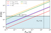Fig. 6. Relation between the rotation period Prot and the magnetic field B introduced in each free precession model. The vertical dashed line shows Prot = 2 s. It is seen that when Prot = 2 s, only the model caused by the internal magnetic field can fit the observation of Bint ≲ 1013.5 − 1014.5 G by adjusting the value of k.

For the radiation-driven precession model, according to Eq. (20), when B_int ≲ 10^14.5 G, the rotation period of the magnetar of FRB 180916 should satisfy P_rot ≲ 0.25 s, which is not consistent with the fourth observation of P_rot = 2 s.

For the fall-back disk precession model, if the eccentricity is caused by the strong magnetic field, according to Eq. (26), we find that the corresponding rotation period needs to satisfy $P_{\mathrm{rot}}\lesssim 0.02\mathrm{s}\frac{M_{\theta }}{0.1M_{\odot }}$. If we set P_rot = 2 s, the initial mass of the fall-back disk should satisfy M_θ ≳ 10 M_⊙, which is not consistent with range of 10⁻⁶ − 10⁻¹ M_⊙.

In summary, for FRB 180916, the free precession model, the radiation-driven precession model, the fall-back disk precession model caused by the strong magnetic field, and the rotation period model are not consistent with these two observations.

4. Summary and discussion

In this paper, we use some recent observations to test several period models for FRB 180916. The geodetic precession model is the most likely periodic model for FRB 180916. The periodic models can also be tested by comparing the difference in the rate of change of the observed period predicted by various models. For the orbital period model, the observed period will be constant. For the free precession model, the radiation-driven precession model, and the rotation period model, the observed period will increase over time. For the geodetic precession model, the observed period will decrease over time. For the fall-back disk precession model, the observed period will increase or decrease over time. Therefore, in the future, we can further test the geodetic precession model by using this characteristic.

Moreover, if we do not consider the fourth observation of Sect. 2, the free precession model caused by internal magnetic field, the radiation-driven precession model, the geodetic precession model, and the fall-back disk precession model can fit other observations. We can further test these models using the observed phase shift over longer observation times in the future. With increasing observation times and data, several periodic models introduced in this paper can be further limited using the above methods. If more periodic FRBs are found, their models can also be tested by imitating the above process.

Acknowledgments

We thank the anonymous referee for helpful comments. This work was supported by the National Natural Science Foundation of China (grant No. U1831207), and the Fundamental Research Funds for the Central Universities (No. 0201-14380045).

References

All Figures

	Fig. 1. Constraint on the internal magnetic field Bint according to Eq. (1). The green line shows the condition of Rm = 106 cm. The colored area represents the allowed range of the internal magnetic field when the value of τd is from 103 s to 105 s.
In the text

Fig. 2. Relation between the internal magnetic field Bint and the numerical coefficient k is drawn according to Eq. (9). The black horizontal line represents the maximum value of the internal magnetic field limited by Eq. (2) when the magnetosphere radius Rm = 106 cm. In addition, the green lines show the relationship between Bint and k drawn from Eq. (9). We show two different conditions, Bdip ∼ 0.1 Bint and Bdip ∼ Bint. The colored area shows the allowable region.

In the text

Fig. 3. Relation between the internal magnetic field Bint and the angle θ is drawn according to Eq. (22). We set θ = θm which means the magnetic axis of the neutron star is aligned in the direction of the dipole axis. The black horizontal lines represent the maximum value of the internal magnetic field limited by Eq. (2). We show two conditions, which are Bint = 1014.5 G and Bint = 1013.5 G. Also, the green lines show the relationship between Bint and θ drawn from Eq. (22). Two different conditions are shown, Bint ∼ 10 Bdip and Bint ∼ Bdip. The colored areas show the allowable region.

In the text

	Fig. 4. Relationship between the mass of the neutron star M1 and q drawn according to Eq. (25), as shown in blue line. The black horizontal solid line represents M1 = 1.4 M⊙ and the black vertical solid line shows q = 1. The blue area of this plot shows the area that matches the observation.
In the text

Fig. 5. Relation between the phase shift Δϕ and the observation duration T for FRB 180916 by combining Eq. (1) with Eq. (2) in different models. The orange and yellow lines represent an upper limit and the blue dashed line represents a lower limit. The colored area can fit the observation. The solid vertical line shows T = 2.2 yr. The rotation period model does not fit the observation of |Δϕ|≲0.3 radian. The two dashed parallel lines mean Δϕ = 1 radian and Δϕ = 0.3 radian, respectively. These models can be tested by verifying whether or not there will be a detectable phase shift within a longer observation duration.

In the text

	Fig. 6. Relation between the rotation period Prot and the magnetic field B introduced in each free precession model. The vertical dashed line shows Prot = 2 s. It is seen that when Prot = 2 s, only the model caused by the internal magnetic field can fit the observation of Bint ≲ 1013.5 − 1014.5 G by adjusting the value of k.
In the text

References

- Beloborodov, A. M. 2020, ApJ, 896, 142 [NASA ADS] [CrossRef] [Google Scholar]
- Beniamini, P., Wadiasingh, Z., & Metzger, B. D. 2020, MNRAS, 496, 3390 [NASA ADS] [CrossRef] [Google Scholar]
- Bochenek, C. D., Ravi, V., Belov, K. V., et al. 2020, Nature, 587, 59 [NASA ADS] [CrossRef] [Google Scholar]
- Chen, H.-Y., Gu, W.-M., Sun, M., Liu, T., & Yi, T. 2021, ApJ, 921, 147 [NASA ADS] [CrossRef] [Google Scholar]
- Cheng, Y., Zhang, G. Q., & Wang, F. Y. 2020, MNRAS, 491, 1498 [NASA ADS] [CrossRef] [Google Scholar]
- CHIME/FRB Collaboration (Amiri, M., et al.) 2020a, Nature, 582, 351 [NASA ADS] [CrossRef] [Google Scholar]
- CHIME/FRB Collaboration (Andersen, B. C., et al.) 2020b, Nature, 587, 54 [Google Scholar]
- Cordes, J. M., & Chatterjee, S. 2019, ARA&A, 57, 417 [NASA ADS] [CrossRef] [Google Scholar]
- Cruces, M., Spitler, L. G., Scholz, P., et al. 2021, MNRAS, 500, 448 [Google Scholar]
- Dai, Z. G., & Zhong, S. Q. 2020, ApJ, 895, L1 [NASA ADS] [CrossRef] [Google Scholar]
- Ghosh, P. 2007, Rotation and Accretion Powered Pulsars (Singapore: World Scientific Publishing Company), 10 [CrossRef] [Google Scholar]
- Hessels, J. W. T., Spitler, L. G., Seymour, A. D., et al. 2019, ApJ, 876, L23 [Google Scholar]
- Hilmarsson, G. H., Michilli, D., Spitler, L. G., et al. 2021, ApJ, 908, L10 [NASA ADS] [CrossRef] [Google Scholar]
- Ioka, K., & Zhang, B. 2020, ApJ, 893, L26 [NASA ADS] [CrossRef] [Google Scholar]
- Josephy, A., Chawla, P., Fonseca, E., et al. 2019, ApJ, 882, L18 [NASA ADS] [CrossRef] [Google Scholar]
- Katz, J. I. 2016, ApJ, 826, 226 [CrossRef] [Google Scholar]
- Katz, J. I. 2021a, MNRAS, 501, L76 [CrossRef] [Google Scholar]
- Katz, J. I. 2021b, MNRAS, 502, 4664 [CrossRef] [Google Scholar]
- Kulkarni, S. R., Ofek, E. O., Neill, J. D., Zheng, Z., & Juric, M. 2014, ApJ, 797, 70 [NASA ADS] [CrossRef] [Google Scholar]
- Levin, Y., Beloborodov, A. M., & Bransgrove, A. 2020, ApJ, 895, L30 [NASA ADS] [CrossRef] [Google Scholar]
- Li, C. K., Lin, L., Xiong, S. L., et al. 2021a, Nat. Astron., 5, 378 [NASA ADS] [CrossRef] [Google Scholar]
- Li, D., Wang, P., Zhu, W. W., et al. 2021b, Nature, 598, 267 [CrossRef] [Google Scholar]
- Li, Q.-C., Yang, Y.-P., Wang, F. Y., et al. 2021c, ApJ, 918, L5 [NASA ADS] [CrossRef] [Google Scholar]
- Lorimer, D. R., Bailes, M., McLaughlin, M. A., Narkevic, D. J., & Crawford, F. 2007, Science, 318, 777 [Google Scholar]
- Lyubarsky, Y. 2014, MNRAS, 442, L9 [Google Scholar]
- Lyutikov, M., Barkov, M. V., & Giannios, D. 2020, ApJ, 893, L39 [NASA ADS] [CrossRef] [Google Scholar]
- Marcote, B., Nimmo, K., Hessels, J. W. T., et al. 2020, Nature, 577, 190 [NASA ADS] [CrossRef] [Google Scholar]
- Margalit, B., & Metzger, B. D. 2018, ApJ, 868, L4 [NASA ADS] [CrossRef] [Google Scholar]
- Mereghetti, S., Savchenko, V., Ferrigno, C., et al. 2020, ApJ, 898, L29 [Google Scholar]
- Metzger, B. D., Margalit, B., & Sironi, L. 2019, MNRAS, 485, 4091 [NASA ADS] [CrossRef] [Google Scholar]
- Michilli, D., Seymour, A., Hessels, J. W. T., et al. 2018, Nature, 553, 182 [Google Scholar]
- Murase, K., Kashiyama, K., & Mészáros, P. 2016, MNRAS, 461, 1498 [NASA ADS] [CrossRef] [Google Scholar]
- Nimmo, K., Hessels, J. W. T., Keimpema, A., et al. 2021, Nat. Astron., 5, 594 [NASA ADS] [CrossRef] [Google Scholar]
- Oostrum, L. C., Maan, Y., van Leeuwen, J., et al. 2020, A&A, 635, A61 [NASA ADS] [CrossRef] [EDP Sciences] [Google Scholar]
- Pastor-Marazuela, I., Connor, L., van Leeuwen, J., et al. 2021, Nature, 596, 505 [NASA ADS] [CrossRef] [Google Scholar]
- Petroff, E., Hessels, J. W. T., & Lorimer, D. R. 2019, A&ARv, 27, 4 [NASA ADS] [CrossRef] [Google Scholar]
- Pleunis, Z., Michilli, D., Bassa, C. G., et al. 2021, ApJ, 911, L3 [NASA ADS] [CrossRef] [Google Scholar]
- Qiao, G. J., Xue, Y. Q., Xu, R. X., Wang, H. G., & Xiao, B. W. 2003, A&A, 407, L25 [NASA ADS] [CrossRef] [EDP Sciences] [Google Scholar]
- Rajwade, K. M., Mickaliger, M. B., Stappers, B. W., et al. 2020, MNRAS, 495, 3551 [NASA ADS] [CrossRef] [Google Scholar]
- Ridnaia, A., Svinkin, D., Frederiks, D., et al. 2021, Nat. Astron., 5, 372 [NASA ADS] [CrossRef] [Google Scholar]
- Sang, Y., & Lin, H.-N. 2022, MNRAS, 510, 1801 [Google Scholar]
- Sob’yanin, D. N. 2020, MNRAS, 497, 1001 [CrossRef] [Google Scholar]
- Spitler, L. G., Scholz, P., Hessels, J. W. T., et al. 2016, Nature, 531, 202 [NASA ADS] [CrossRef] [Google Scholar]
- Tavani, M., Verrecchia, F., Casentini, C., et al. 2020, ApJ, 893, L42 [NASA ADS] [CrossRef] [Google Scholar]
- Tavani, M., Casentini, C., Ursi, A., et al. 2021, Nat. Astron., 5, 401 [NASA ADS] [CrossRef] [Google Scholar]
- Tendulkar, S. P., Gil de Paz, A., Kirichenko, A. Y., et al. 2021, ApJ, 908, L12 [CrossRef] [Google Scholar]
- Tong, H., Wang, W., & Wang, H.-G. 2020, Res. Astron. Astrophys., 20, 142 [Google Scholar]
- Wada, T., Ioka, K., & Zhang, B. 2021, ApJ, 920, 54 [NASA ADS] [CrossRef] [Google Scholar]
- Wadiasingh, Z., & Timokhin, A. 2019, ApJ, 879, 4 [NASA ADS] [CrossRef] [Google Scholar]
- Wang, F. Y., & Yu, H. 2017, JCAP, 03, 023 [CrossRef] [Google Scholar]
- Wang, F. Y., Wang, Y. Y., Yang, Y.-P., et al. 2020, ApJ, 891, 72 [NASA ADS] [CrossRef] [Google Scholar]
- Wei, J.-J., Wu, X.-F., Dai, Z.-G., et al. 2021, ApJ, 920, 153 [NASA ADS] [CrossRef] [Google Scholar]
- Xiao, D., Wang, F.-Y., & Dai, Z.-G. 2021, Sci. China Phys. Mech. Astron., 64, 249 [Google Scholar]
- Xu, K., Li, Q.-C., Yang, Y.-P., et al. 2021, ApJ, 917, 2 [NASA ADS] [CrossRef] [Google Scholar]
- Yang, H., & Zou, Y.-C. 2020, ApJ, 893, L31 [NASA ADS] [CrossRef] [Google Scholar]
- Zanazzi, J. J., & Lai, D. 2020, ApJ, 892, L15 [NASA ADS] [CrossRef] [Google Scholar]
- Zhang, B. 2020, Nature, 587, 45 [CrossRef] [Google Scholar]
- Zhang, G. Q., Wang, P., Wu, Q., et al. 2021, ApJ, 920, L23 [NASA ADS] [CrossRef] [Google Scholar]
- Zhao, Z. Y., Zhang, G. Q., Wang, Y. Y., Tu, Z.-L., & Wang, F. Y. 2021, ApJ, 907, 111 [NASA ADS] [CrossRef] [Google Scholar]