| Issue |
A&A
Volume 658, February 2022
|
|
|---|---|---|
| Article Number | A40 | |
| Number of page(s) | 20 | |
| Section | Planets and planetary systems | |
| DOI | https://doi.org/10.1051/0004-6361/202142286 | |
| Published online | 28 January 2022 | |
How does the background atmosphere affect the onset of the runaway greenhouse?
1
Observatoire de Genève, Université de Genève,
Chemin Pegasi 51b,
1290
Sauverny, Switzerland
e-mail: This email address is being protected from spambots. You need JavaScript enabled to view it.
2
Laboratoire d’astrophysique de Bordeaux, Univ. Bordeaux, CNRS, B18N, allée Groffroy Saint-Hilaire,
Pessac,
33615, France
Received:
23
September
2021
Accepted:
27
October
2021
Abstract
As the insolation of an Earth-like (exo)planet with a large amount of water increases, its surface and atmospheric temperatures also increase, eventually leading to a catastrophic runaway greenhouse transition. While some studies have shown that the onset of the runaway greenhouse may be delayed due to an overshoot of the outgoing longwave radiation (OLR) – compared to the Simpson-Nakajima threshold – by radiatively inactive gases, there is still no consensus on whether this is occurring and why. Here, we used a suite of 1D radiative-convective models to study the runaway greenhouse transition, with particular emphasis on taking into account the radical change in the amount of water vapour (from trace gas to dominant gas). The aim of this work is twofold: first, to determine the most important physical processes and parametrisations affecting the OLR; and second, to propose reference OLR curves for N2+H2O atmospheres. Through multiple sensitivity tests, we list and select the main important physical processes and parametrisations that need to be accounted for in 1D radiative-convective models to compute an accurate estimate of the OLR for N2+H2O atmospheres. The reference OLR curve is computed with a 1D model built according to the sensitivity tests. These tests also allow us to interpret the diversity of results already published in the literature. Moreover, we provide a correlated-k table able to reproduce line-by-line calculations with high accuracy. We find that the transition between an N2-dominated atmosphere and an H2O-dominated atmosphere induces an overshoot of the OLR compared to the (pure H2O) Simpson–Nakajima asymptotic limit. This overshoot is first due to a transition between foreign and self-broadening of the water absorption lines, and second to a transition between dry and moist adiabatic lapse rates.
Key words: planets and satellites: terrestrial planets / planets and satellites: atmospheres
© ESO 2022
1 Introduction
Terrestrial planets can retain liquid water at their surface when the absorbed stellar radiation is balanced by the thermal emitted flux. If this balance is broken and if the absorbed flux is the highest, the planet warms to reach a new stable state at a higher temperature. Due to the strong opacity of water in the infrared, the thermal emission can be fully absorbed by the atmosphere when the temperature is high enough. Consequently, the thermal emission reaches a maximum, named the Simpson-Nakajima limit (Simpson 1929; Nakajima et al. 1992). Therefore, the planet stays in an unstable state and a catastrophic positive feedback arises and dramatically increases its temperature.
There is a strong interest to study this runaway greenhouse effect (Komabayasi 1967; Ingersoll 1969; Kasting 1988; Nakajima et al. 1992; Goldblatt & Watson 2012; Boukrouche et al. 2021), in particular to accurately determine the Simpson-Nakajima limit. This would allow us to know how close the Earth is to the runaway greenhouse threshold, but also to determine the inner edge of the habitable zone (HZ) more precisely (e.g. Kasting et al. 1993; Kopparapu et al. 2013; Zhang & Yang 2020). Some studies (e.g. Goldblatt et al. 2013; Kopparapu et al. 2014; Ramirez 2020) have shown that the outgoing longwave radiation (OLR) may be strongly modified by radiatively inactive gases (e.g. N2 or O2, as in the Earth’s atmosphere). Other studies (Pierrehumbert 2010; Koll & Cronin 2019) have shown that such gases may lead to an overshoot of the Simpson-Nakajima limit, thus delaying the runaway greenhouse positive feedback. These OLR values, overshot compared to the pure water runaway greenhouse, are interpreted in Pierrehumbert (2010) as a coupled effect of the pressure broadening – which increases the absorption – and a lapse rate – which shifts towards a dry adiabatic lapse rate, thus reducing the absorption. Kopparapu et al. (2013) also suggested that the differences could come from the parametrisation of the adiabatic lapse rate. Kopparapu et al. (2013) used the Kasting (1988) formulation, while other papers used the Ding & Pierrehumbert (2016) formulation. Moreover, Koll & Cronin (2019) interpreted the OLR overshoot as a modification of the scale height of the atmosphere due to a change of the mean molecular weight. Possible interpretations are multiple, but there is still no consensus in the literature as of whether an OLR overshoot is really expected or not (see Fig. 1). The Simpson–Nakajima limit is quite well constrained for a pure vapour atmosphere (see Fig. 1, first panel), but differences between the various studies appear even with 0.1 bar of N2, and reach up to 35 W m−2 for 10 bar of N2. These discrepancies increase with the nitrogen pressure. Thus, at least one important process may be unknown - or not well constrained - to accurately compute the OLR of such atmospheres.
The first aim of this work is to determine, through sensitivity tests, the main physical processes and parametrisations involved in the computation of the OLR with a 1D radiative-convective model. This can be useful to better constrain 3D GCM simulations through a better understanding of some of the main physical processes that may be at play. Secondly, we propose a reference OLR curve (Fig. 3, top panel), done with a model built according to the sensitivity tests, for a H2O + N2 atmosphere,and to solve the question of the potential overshoot. We also propose a H2O + N2 correlated-k table, which provides similar results as a line-by-line computation.
In this work, we used a suite of 1D radiative-convective models already described in the literature. These models, presented in Table 1 (see also Sect. 2.3), are composed of a convection scheme and a radiative transfer model. For this reason, in the method section (Sect. 2) we firstly introduce different convection schemes (Sect. 2.1) and radiative transfer methods (Sect. 2.2), and finally we present the set of models we used (Sect. 2.3). We present our results in Sect. 3 and we discuss them in Sect. 4. We provide our conclusions in Sect. 5.
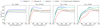 |
Fig. 1 OLR as a function of surface temperature for different N2 partial pressures ( |
Main characteristics of 1D radiative-convective models used in this work.
2 Method
With the aim of reconciling the large range of results proposed in the literature (Fig. 1), we explored physical mechanisms induced by the addition of nitrogen in a pure steam atmosphere. We built a line-by-line 1D radiative-convective model usable as reference model, named PyRADS-Conv1D, to compute the OLR of the atmosphere. The radiative transfer calculation is derived from the PyRADS1 model (Koll & Cronin 2018), and the convective scheme is derived from the RADCONV1D model (Marcq et al. 2017).
To be confident with the physical processes to be included in PyRADS-Conv1D, we performed multiple sensitivity tests using different convective schemes (Sect. 2.1) and radiative transfer methods (Sect. 2.2) from 1D models already described in the literature and presented in Table 1. An exhaustive list of these tested processes and parametrisations is presented below (see also Table A.1). The complete overview of the impact of each parametrisation on the OLR value is available in Appendix A. A similar comparison was done by Yang et al. (2016) with other 1D models, and they found the same wide range of results. More precisely, they show that differences appear using similar models and they explain that these differences are mainly induced by the choice of the water continuum. Our more detailed sensitivity tests were motivated by the interesting conclusions of this study. We tested the following parametrisations: (1) the convection scheme, (2) the resolution of the vertical grid, (3) the shape of the absorption lines, (4) the spectral resolution of the absorption spectrum, (5) a self- of foreign broadening of the absorption lines, (6) the quantity of water isotopes, (7) the truncation of the water continuum, (8) with or without the H2O-N2 continuum, (9) the version of the H2O-H2O and H2O-N2 continua, (10) with or without the N2 –N2 Collision Induced Absorption (CIA) continuum, (11) the effect an additional fixed amount of CO2, (12) the solution of the two-stream equations, (13) the interpolation scheme of the correlated-k method.
2.1 Convection schemes
The atmospheres we studied are made of a variable amount of condensable gas (water) and a fixed amount of background gas (nitrogen). The quantity of each gas in the atmospheric layer is dictated by the surface temperature and the surface partial pressures and following a moist adiabatic lapse rate (hereafter ‘moist adiabat’). Generally, we assume that condensates are immediately removed by precipitation. This pseudo-adiabatic hypothesis is motivated by the fact that 1D models lack a self-consistently calculated description of (inherently 3D) cloud formation and thus precipitation. Consequently, these models are considered cloud free without other assumptions. The atmospheric profiles are assumed to be fully saturated, and thus the pressure of the condensable gas (here water) is equal to the saturation pressure. In other words, the relative humidity (RH) is equal to unity except in the stratosphere.
The main moist adiabats provided by (and used in) the literature are proposed by Kasting (1988) and Ding & Pierrehumbert (2016). An analytic comparison is made in Appendix B, and it highlights that the main difference between them is the assumption used to define the entropy of the condensable gas. With the aim of comparing and discussing the assumptions and parametrisations done to compute the atmospheric profiles of 1D radiative-convective models, we used two different convective schemes in our study, which are based on the two different adiabats of the literature. The first one, Conv_K88, is based on the adiabat proposed in Kasting (1988), and the second one, Conv_D16, uses the adiabat proposed in Ding & Pierrehumbert (2016). These schemes also assume two different definitions of the vertical grid (see Appendix A.2.1). A complete description of these schemes is given here.
The temperature profiles made by the Conv_K88 scheme follow a lapse rate computed using the equation from Kasting (1988) with 200 atmospheric levels and a minimum total pressure at the top fixed at 0.1 Pa. The saturation pressure and the water entropy are computed using experimental look-up tables (Haar et al. 1984). When the temperature reaches 200 K, the atmosphere is considered isothermal with a constant water-mixing ratio (Kasting et al. 1993). The change of gravity in the atmosphere due to the altitude is taken into account. This method was developed for RADCONV1D (Marcq et al. 2017).
The Conv_D16 scheme uses the Ding & Pierrehumbert (2016) adiabatic lapse rate, with 100 levels and a fixed pressure difference between the top and the bottom of the atmosphere (106 Pa). The pressure of the highest level is not fixed, but the two previous parameters are interdependent and chosen to correctly represent the whole atmosphere (see Appendix A.2.1 for more details). The saturation pressure is computed using the Clausius-Clapeyron equation. By definition of the Ding & Pierrehumbert (2016) formulation of the adiabatic lapse rate, the water entropy is computed using the perfect gas approximation (see Appendix B). When the temperature reaches 150 K, the atmosphere is considered isothermal and the water-mixing ratio is fixed. This method was developed for PyRADS and the original parameters are available in Koll & Cronin (2018).
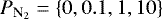
We fixed the number of atmospheric levels of each method thanks to a test of convergence of the OLR value relative to the vertical resolution (see Appendix A.2.1). Figure 2 highlights differences of the thermal profiles and of the water-mass-mixing ratio profiles computed using one convection scheme or the other. The Conv_K88 scheme is more accurate because it is based on look-up tables, while the Conv_D16 scheme is based on perfect gas equations (e.g. Clausius–Clapeyron equation). This induces a non-negligible difference on the estimation of the OLR value (Fig. A.7). For this reason, we used the Conv_K88 scheme as a reference convective scheme (see Sect. 2.3). Figure 2 also shows that for a high surface temperature, that is a high surface pressure, the Conv_D16 scheme is not able to represent the stratosphere because of the fixed difference of pressure between the top and the bottom of the atmosphere.For both methods, we considered an Earth-like planet with a gravity acceleration at the surface equal to 9.81 m s−1.
It is important to keep in mind that for both convection schemes presented in this work the pseudo-adiabatic hypothesis induces a water pressure equal to the saturation pressure (i.e. given by the temperature). Therefore, as the surface boundary conditions are fixed (temperature and nitrogen pressure), the surface water pressure stays unchanged whatever the background gas pressureis.
2.2 Radiative transfer methods
In this work, we used different radiative transfer methods from four different models presented in Table 1. These methods aresub-divided between the two families of radiative transfer calculations detailed below: line-by-line and correlated-k.
PyRADS-RT and PyRADS-updated are line-by-line methods, while kcm1d-RT and Exo_k-RT are correlated-k methods. Our aim here is to use a line-by-line method, through the PyRADS-Conv1D model, to produce a result as accurate as possible to benchmark the calculations performed using a correlated-k method, which is computationally much more efficient. We used Exo_k as reference model for the correlated-k method. This approach is motivated by the large dispersion of results in the literature and to reconcile line-by-line and correlated-k studies, which seemingly lead to different results (Fig. 1).
The specificities of the line-by-line and correlated-k methods are detailed below. Several sensitivity tests were performed to quantify theinfluence of each of the assumptions usually done in the literature on the final estimation of the OLR (Appendix A).
As shown in Table 1, for all methods the H2O-H2O and H2O-N2 continua are taken into account using the MT_CKD database (Mlawer et al. 2012). The N2 –N2 collision-induced absorption (CIA) is taken from the HITRAN CIA database (Karman et al. 2019). According to the MT_CKD formalism (Mlawer et al. 2012) the water vapour absorption lines are truncated at 25 cm−1 and the plinth2 is removed from the line centre calculation. In PyRADS-updated, we use the MT_CKD3.2 continuum as explained in Appendix A.1.2. We choose to include only the main isotope water absorption lines in the radiative transfer calculation of PyRADS-updated to increase the computation speed. This is also motivated by our of knowledge of the typical isotopic fraction of the water on terrestrial exoplanets. This assumption does not significantly change the final result (see Appendix A.1.3). Finally, to compute the pressure broadening of the lines we need to have the exponents that describe the temperature dependence for N2 and H2O (see Eq. (1)). The exponent for N2 was taken equal to that of the (Earth) ‘air’ composition (Gordon et al. 2017). We do not include Rayleigh scattering by water vapour for either methods because it becomes important beyond 10000 cm−1 (Kopparapu et al. 2013) where the thermal emission (i.e. the Planck law) is null for the studied range of temperature.
The radiative methods presented here assume different approximations to solve the two-stream equations used to describe the radiative transport of an atmosphere through a upward and downward flux (Meador & Weaver 1980). The kcm1d-RT method uses the classical hemispheric mean approximation while PyRADS-RT and PyRADS-updated and Exo_k-RT assume  with
with  . This approximation is only valid in the context of a non-scattering atmosphere.
PyRADS-RT and PyRADS-updated assume  which yields less than 1 W m−2 of difference compared to the modified hemispheric mean method (see Appendix A.1.5 for more details).
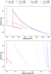 |
Fig. 2 Comparison between Conv_K88 (full lines) and Conv_D16 (dotted lines) convection schemes for different surface temperatures. The top panel represents the temperature profiles, and the bottom panel represents the volume-mixing ratio of the water for different surface temperatures. Here,
|

2.2.1 Line-by-line method
The most direct radiative transfer method is to compute the exact absorption spectrum at each level of the atmosphere, that is for each pressure to temperature couple. In other words, the line-by-line method computes the absorption at each wavelength while the correlated-k method considers a statistical distribution of the absorption spectrum. This method avoids interpolations of spectra intrinsic to the correlated-k computation and allows greater flexibility relative to the composition of the atmosphere. However, it makes the computation more time-expensive. As line-by-line computations provide an exact result, we chose PyRADS-updated as a reference radiative transfer method.
The PyRADS-RT and PyRADS-updated methods (Table 1) use low-resolution spectra computed using the HITRAN 2016 line list (Gordon et al. 2017) and assume the shape of the lines follows a Lorentz profile. We show in the Appendix that a spectral resolution of 0.01 cm−1 is sufficient to keep a high accuracy, in agreement with Koll & Cronin (2018). We adapted the PyRADS-RT method to create the PyRADS-updated method by adding the N2 –N2 CIA computation from PyRADS-shortwave3 (Koll & Cronin 2019) and using a version of MT_CKD continuum extended up to 20 000 cm−1 (see Table 1).
2.2.2 Correlated-k method
Models based on the correlated-k method (Fu & Liou 1992) are convenient to use because of their much shorter computation time. Here, absorption spectra are pre-computed for pressure, temperature, and mixing ratio reference values in a so-called correlated-k table. During the radiative transfer calculation, a statistical wavelength distribution of these spectra is interpolated (e.g. Fu & Liou 1992; Leconte 2021) on the pressure to temperature values of each atmospheric level. The correlated-k method can in principle provide the same results as a line-by-line calculation, but at a much lower computational cost. To achieve this purpose the number of bands of the correlated-k table needs to be high enough, as well as the resolution of the pressure, temperature, and mixing ratio grids. In this paper, we provide an H2O + N2 table that gives similar results to an exact calculation (Fig. 3, top panel).
To build the correlated-k table used in this work, we computed a dataset of high-resolution spectra using the HITRAN 2016 database (Gordon et al. 2017). These spectra are calculated for multiple values of temperature (T = {50, 110, 170… 710, 5000} K), pressure (P ={0.1, 1, 10…107} Pa), and water-mass-mixing ratio (Q = {10−6, 10−5, 10−4…1}). The 21 Gauss points of the table follow a Legendre distribution. The infrared (IR) band is defined in the [10; 4000] cm−1 range with a resolution R = 8 (48 bands), which is sufficient to accurately compute water absorption spectra. We also include absorption lines of the water isotopes at terrestrial abundances (De Biévre et al. 1984) in the absorption spectra, but as shown in Appendix A.1.3 this does not significantly change the OLR value. We share the correlated-k table used in this work4 for a larger spectral range ([0.1; 30000] cm−1) and a higher resolution (R = 300). A usable table at lower resolution can easily be made by using the Exo_k package5.
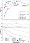 |
Fig. 3 OLR as a function of the surface temperature (top panel) or as a function of the nitrogen pressure (bottom panel). The top panel represents the OLR curve for different N2 pressures (black: |


2.3 Description of the models
Every 1D radiative convective model presented in Table 1 is composed of a convection scheme and a previously described radiative transfer method. The models used are presented here.
The 1D reverse version of LMD-Generic, also named kcm1d (Turbet et al. 2019), uses the Conv_K88 scheme (developed for RADCONV1D; Marcq et al. 2017) and the kcm1d-RT radiative transfer method. This method, described above, is derived from the LMD-Generic model and includes some GCM-specific parametrisations (see Appendices A.1.5 and A.2.4).
The Exo_k model (Leconte 2021) also uses the Conv_K88 scheme. Its radiative transfer method, Exo_k-RT is a correlated-k method that provides results in accordance with our reference model PyRADS-Conv1D (see top panel in Fig. 3). For this reason, we use it as reference model for sensitivity tests related to the correlated-k method.
The PyRADS model (Koll & Cronin 2018) uses the Conv_D16 scheme with the PyRADS-RT method. We adapted several parameters to fit our needs (e.g. the vertical grid, see Appendix A.2.1). The original parameters are available in Koll & Cronin (2018).
We built the PyRADS-Conv1D model using the most accurate convection scheme (Conv_K88) and radiative transfer method (PyRADS-updated) to produce reference OLR curves according to our sensitivity tests.
3 Results
We present our results in this section. First, we describe the processes that induce a runaway greenhouse effect for a pure steam atmosphere (Sect. 3.1). Secondly, we highlight the differences that arise by adding nitrogen and the processes that allow the OLR overshoot relative to the Simpson-Nakajima limit (Sect. 3.2). Finally, we discuss the two physical processes that induce the overshoot of the OLR in detail (Sects. 3.3.1 and 3.3.2).
3.1 Runaway greenhouse of a pure water atmosphere
The global physical processes that induce a runaway greenhouse effect for a pure water atmosphere are now very well constrained (Ingersoll 1969; Nakajima et al. 1992; Goldblatt & Watson 2012), but numerical estimations of the value of the greenhouse asymptotic limit vary between the different studies, as shown in Fig. 1. These small differences may come from the assumptions made in models or from second-order neglected processes. To understand origins of these differences, we first describe the physical processes involved in a warming atmosphere.
Consider an Earth-like rocky (exo)planet with a global ocean without background gases. At very low temperatures, typically lower than 290K, almost all water is condensed or solidified at the surface of the planet; thus, the (H2O-dominated) atmosphere is very thin and the planet radiates similarly to a black body. If the surface temperature increases, the thermal emission increases because of the Planck radiation law, and the surface water is expected to progressively evaporate. The thin water vapour atmosphere induces a greenhouse effect via IR absorption by water vapour, consequently the OLR is not strictly equal to the black body emission law. If the temperature increases again, the surface pressure reaches a limit, Pthick, for which the atmosphere becomes optically thick at long wavelengths (i.e. in the IR absorption bands of water). The OLR is then decoupled from the surface temperature (Nakajima et al. 1992; Pierrehumbert 2010; Goldblatt et al. 2013; Boukrouche et al. 2021). As the temperature profile follows a purely wet adiabat, the structure of the atmosphere in the thin layers (i.e. ‘radiatively active layers’ from the optically thick limit Pthick) up to the top stay unchanged by increasing the surface temperature (see blue curves, i.e. high temperatures, in Fig. 2). Therefore, the absorption in these layers also remains unchanged. For this reason, the OLR reaches an asymptotic limit known as the moist troposphere limit or the Simpson–Nakajima limit (Goldblatt & Watson 2012). As a result, if the absorbed stellar radiation (ASR) is higher than this asymptotic limit, the radiative balance is broken and the surface temperature increases, inducing even more evaporation and progressively building up a thick water-steam-dominated atmosphere. This is the runaway greenhouse effect. When the entire ocean is evaporated and when the planet reaches extremely high temperatures of thousands of kelvins (e.g. Kasting et al. 1993; Kopparapu et al. 2013; Turbet et al. 2019), the OLR increases again. For these temperatures, the planet radiates in the visible, where the water is optically thin.
3.2 Runaway greenhouse of an H2O + N2 atmosphere: the overshoot effect
In this section, we describe physical processes that may lead to or prevent an OLR overshoot, presented in the top panel of Fig. 3, for an H2O + N2 atmosphere and computed with PyRADS-Conv1D and Exo_k. Regarding Figs. 4 and 5, the evolution of the OLR value is mainly determined by the water-volume-mixing ratio value, whatever the nitrogen pressure, according to three ranges of mixing ratio values: below 5 × 10⁻⁵, between 5 × 10⁻⁵ and 0.2, and above 0.2. Therefore, in the following we describe the evolution of the OLR through three cases: low, high, or intermediate mixing ratios.
At very low mixing ratios, the surface temperature is rather low (Fig. 4). Consequently, the vapour pressure is also low and N2 is dominant;thus, the lapse rate is very close to a dry adiabatic lapse rate. For the following, we assumed a dry adiabat. Moreover, the broadening of the water absorption lines is dominated by foreign broadening (Fig. 6).
The atmospheric absorption is mainly in the first layers that contain water (with a partial water pressure roughly greater than 5 Pa). The temperature of a dry atmosphere is lower than for a wet one, that is the temperature decreases faster relatively to altitude (Fig. 2). Therefore, for a given low surface temperature, the total amount of steam in the whole atmosphere is low if the nitrogen pressure is high (because the lapse rate is close to a dry adiabatic lapse rate; see Fig. 4); thus, the intensity of absorption lines decreases by increasing the nitrogen pressure (e.g. bottom panel of Fig. 3 for Tsurface = 275 K). However, as the vapour pressure is limited by the pseudo-adiabatic hypothesis, it cannot exceed the saturation pressure ( ); therefore, the self-broadening is limited as well. As nitrogen is a non-condensable gas here, its pressure is not limited and the foreign broadening may be stronger than the self-broadening. Therefore, when the atmosphere is nitrogen dominated, the total broadening of the absorption lines is stronger than for a pure vapour atmosphere, the atmosphere absorbs in more wavelengths, and the OLR is weaker than for a pure vapour atmosphere, as shown in the bottom panel of Fig. 3 and for the
  =10 bar in the top panel of Fig. 3.
At high mixing ratios, the temperature is high and water becomes dominant; hence, the temperature profile follows a moist adiabatic lapse rate. By evaporating more and more water, the absorption line broadening becomes dominated by the self-coefficient, and the mean molecular weight tends towards the water molecular weight. Properties of the atmosphere (temperature profile, mixing ratio, molecular weight, etc.) tend towards the properties of a pure water atmosphere; thus, the OLR tends towards the Simpson–Nakajima limit (Fig. 3, bottom panel).
At intermediate mixing ratios (the OLR overshoot), the corresponding intermediate temperatures corresponds to the transition between an N2 -dominated and an H2O-dominated atmosphere (Fig. 4). First, this induces a transition between a foreign broadening and a self-broadening of the water absorption lines. As the self-broadening is stronger than the foreign broadening, the absorption increases strongly during this transition. As shown in Fig. 6, the overshoot itself exists through this broadening transition and may be missed by neglecting the change of broadening species (for more details, see Sect. 3.3.1).
Second, the transition between an N2 -dominated and an H2O-dominated atmosphere induces a transition between a dry and a wet adiabatic lapse rate (Figs. 2 and 7). Even if N2 is still dominant (volume-mixing ratio below 0.2), the water pressure becomes non-negligible (Figs. 4 and 5). Because of that, a small increase in the surface temperature tends to turn the dry adiabatic lapse rate into a wet adiabatic lapse rate. As the adiabat becomes wetter, the structure of the atmosphere changes and the temperature decreases more slowly with the altitude (Fig. 7), which tends to allow more water in the upper layers. This has the effect of increasing the size of the atmosphere strongly and quickly (Fig. 4). Due to this positive feedback effect, the transition of dominant species can be done over a small temperature range (Fig. 7).
Nevertheless, we can see that the transition between wet and dry atmospheres spans a wider temperature range for higher nitrogen pressures. If N2 pressure is higher, H2O pressure required to be vapour dominated is higher, and thus the required surface temperature is higher. Therefore, the temperaturedifference between the first visible effects of non-negligible vapour quantity and a vapour-dominated atmosphere is bigger. That is the reason why the overshoot spans a wider temperature range for 10 bar of nitrogen (Fig. 3).
Finally, the transition of dominant species also induces a transition of the mean molecular weight, from nitrogen molecular weight to water molecular weight. As explained in detail in Sect. 3.3.2, changing the mean molecular weight affects both the atmospheric profile and the radiative transfer calculation. Increasing molecular weight of the background gas tends to reduce the R∕cp value, and thus the OLR decreases. On the other hand, increasing the molecular weight of the background gas also tends to reduce the opacity of the atmosphere, and thus the OLR increases. As shown in Fig. 8, this second effect is stronger; therefore, as shown on the bottom panel of the Fig. 8, it increasing the molecular weight of the background gas means increasing the OLR. When water becomes dominant, the mean molecular weight – and all the physical properties of the atmosphere – tend towards water values, and the OLR converges on the Simpson–Nakajima limit. Consequently, the height of the overshoot is mainly determined by the molecular weight of the background gas (nitrogen here), while the overshoot itself is due to the broadening transition.
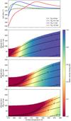 |
Fig. 4 OLR and corresponding atmospheric water content as a function of the surface temperature. The top panel is the OLR as a function of the surface temperature for different nitrogen pressure, computed with PyRADS-Conv1D. The three bottom panels represent the size of the atmosphere (up to 0.1 Pa)for different nitrogen pressures where the colour bar indicates the water-volume-mixing ratio ( |

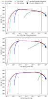 |
Fig. 5 OLR as a function of the volume-mixing ratio for different nitrogen surface pressures using Exo_k. The volume-mixing ratio (vmr) values are given at the top of the atmosphere (top panel), at 0.01 bar (middle panel), and at 0.1 bar (bottom panel) of total pressure. The black cross represent the Simpson-Nakajima limit for a pure vapour atmosphere,and the vertical dashed lines approximately delimit the range of vmr values for which there is a transition of dominantspecies. |
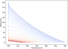 |
Fig. 6 OLR as a function of the temperature for |

3.3 Physical effects of the nitrogen
In this section, we discuss the two main effects of the nitrogen in detail. These are introduced in Sect. 3.2. The first one is the broadening effect (Sect. 3.3.1), and the second one is the mean molecular weight effect (Sect. 3.3.2).
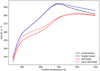 |
Fig. 7 Temperature profiles computed with the Conv_K88 scheme for different surface temperatures with
|

3.3.1 Broadening effect
In radiative transfer calculations, whatever the method used, the half width at half maximum (HWHM) of the absorption lines due to the pressure broadening can be described by Eq. (1) from Gordon et al. (2017):
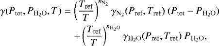 (1)
(1)
where Ptot is the total pressure,  the partial water pressure, and T the temperature.
  and
and  are the HWHM of the foreign- and the self-pressure broadening at the reference temperature. As explained previously, we assume that the nitrogen temperature dependency exponent is equal to the air exponent:
  . This assumption is motivated by the lack of an experimental value for N2 alone, but the difference should be small. For the same reasons, we also assume that the self-component of the pressure-induced shift of the line centre (δ in Gordon et al. 2017) is equal to that of the air component: δself = δAIR.
If the background gas is a trace gas, it is possible to neglect the HWHM of the foreign broadening and assume that the line broadening only depends on the self-broadening (Eq. (2)). However, as explained before, for low surface temperatures the water pressure is limited by the pseudo-adiabatic hypothesis, while the nitrogen pressure is not. Therefore, by only considering the self-broadening to compute the pressure broadening (Eq. (2)), the HWHM and thus the absorption is largely over-estimated, which leads to incorrect OLR values where the overshoot is hardly visible (red lines in Fig. 6):
 (2)
(2)
where Ptot is the total pressure. This effect is strong in our case study because of the transition between an N2 -dominated and an H2O-dominated atmosphere.The black curve in Fig. 6 highlights the transition between the N2 -dominant (i.e. foreign) and the H2O-dominant (i.e. self) broadening, corresponding to the curves proposed in Fig. 3.
It is possible to build a correlated-k table from high-resolution spectra of pure water even by neglecting the foreign broadening. This possibility is commonly used to skip the tedious step of calculating a large number of spectra in the case of a unusual mixof gases. By doing that, we assume a self-broadening only, and thus we over-estimate the absorption (dotted red line in Fig. 6) as explained just above. Regarding our conclusions, the error induced by this method is only negligible if the background gas is a trace gas. However, Amundsen et al. (2017) discussed different possibilities to easily produce correlated-k for mixed gases. They show that in particular cases, correlated-k table built by mixing the tables of pure species, that is by neglecting the mutual broadening, may produce accurate results with a greater flexibility than by creating pre-mixed correlated-k tables.
It can be counter-intuitive to state that an OLR curve produces an overshoot by only assuming the foreign broadening but not by only assuming the self-broadening (Fig. 6). This may be explained by a subtle effect of the broadening power of water and nitrogen. As the self-broadening is stronger than the foreign one, the absorption lines of the ‘self-only case’ are probably already more broadened than for the ‘foreign-only case’. Therefore, the overshoot effect described previously is probably weaker if weonly consider the self-broadening. Nevertheless, a deeper study of this point is needed before any conclusion can be drawn.
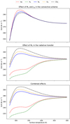 |
Fig. 8 OLR as a function of the surface temperature by only using the physical properties of other gases in the convective scheme calculation (top panel), in the radiative transfer calculation only (middle panel) and in both of them (bottom panel). The full blue line corresponds to the curve presented in the top panel of Fig. 3 with the true value of the nitrogen molecular weight. The dotted lines correspond to Mn and cp values of other gases (see Table 2). Here, we used the Conv_D16 scheme and the Exo_k-RT radiative transfer method assuming 1 bar of background gas. |
3.3.2 Molecular weight effect
As discussed in Pierrehumbert (2010), the addition of a background gas modifies the atmospheric structure, which plays an important role on the shape of the OLR curve. We can study this effect by analysing the effect of the molecular weight of the background gas on the atmospheric profile and on the radiative transfer calculation separately. For convenience and as we only analysed tendencies, we chose to use the Conv_D16 scheme and the Exo_k-RT radiative transfer method. In the same way, radiative properties of the background gas (mainly the broadening) are those of nitrogen in order to only study the effect of the molecular weight on the OLR value.
With regard to the effect on the atmospheric profile, by rewriting the equation proposed by Ding & Pierrehumbert (2016) (see Eq. (B.3)) and assuming a constant number of background molecules (nn), it is possible to show that the adiabatic lapse rate depends on the molecular weight of the background gas (Mn) only through the Rn ∕cpn value (in red in Eq. (3)), where Rn is the specific gas constant of the background gas (Eq. (3)):
 (3)
(3)
Indices of variables in Eq. (3) indicate what gas is considered: c for the condensable gas (water here) and n for the background gas. Here, P is the pressure, T the temperature, M the molecular weight, R* the perfect gas constant, R the specific gas constant, L the latent heat, and cp the heat capacity. By changing the background gas, both Mn and cpn change as shown in Table 2. However, for diatomic gases (N2, O2, H2...), the molecular heat capacity (cp,molec = cp × M) is remarkably similar. By definition, the Rn∕cpn value is also remarkably similar whatever the considered diatomic gas. This means that for such gases, most of the atmospheric profiles will be the same, as will the OLR curve as shown on the top panel of Fig. 8. For triatomic molecules such as CO2, the Rn∕cpn value decreases, which means that the temperature decreases more slowly with altitude. Therefore, the atmosphere warms up and because of the pseudo-adiabatic hypothesis, the total amount of water increases, and the OLR decreases.
Concerning the effect on the radiative transfer, the molecular weight of the background gas has a much stronger impact on the radiative transfer calculation. By assuming a radiatively inactive background gas, the opacity of the atmosphere (τ) can be simply written by Eq. (4):
 (4)
(4)
where xi, σi are the volume-mixing ratio and the cross-sectionper molecule (in m2/molecule) of the species i. NA is the Avogadro number.
Interestingly, if the molecular weight of the background gas (Mn) changes without altering the atmospheric temperature profile (i.e. if Rn∕cpn remains constant), then the vapour-volume-mixing ratio profile does not change either because it only depends on T(p). In other words,at any pressure level, the water-molecule-to-background-gas ratio stays the same. However, rather counter intuitively, changing Mn at a constant surface pressure changes the total number of molecules of background gas, and hence the total number of water molecules, although the ratio and total mass stay the same.
Therefore, for a given atmospheric profile, if the molecular weight of the background gas (Mn) decreases, the mass of water vapour in the atmosphere increases and the latter becomes more opaque, as demonstrated by Eq. (4). This leads to a decrease in the OLR, as shown on the middle panel of Fig. 8.
Concerning the global effect of the molecular weight, as is visible in Fig. 8, the effect of the molecular weight on the radiative transfer calculation (middle panel) is largely dominant compared to the modification of the atmospheric profile (top panel). For this reason, the OLR curve obtained by taking into account both effects (bottom panel) is similar to the one for which we take into account only the effect on the radiative transfer.
For gas mixtures with other inactive gases (e.g. O2, H2), the proposed analysis may help to understand how the OLR evolves regarding changes of the mean molecular weight of the atmosphere. For example, gases lighter than N2 – such as H2 – tend to reduce the OLR, as shown by previous studies (e.g. Koll & Cronin 2019). For radiatively active gases such as CO2, the molecular weight effect still plays a role but may become a second-order process compared to the absorption of the gas itself (see e.g. Appendix A.1.4). However, when changing the mixture, the radiative properties of the atmosphere will change and the OLR will be slightly impacted.
It is interesting to notice that when the global effect of the molecular weight is taken into account (bottom panel on Fig. 8), there is a qualitative change in the shape of the OLR curve, and even a hump when using the He gas properties. This hump, which arises below the Simpson–Nakajima limit, is discussed in Koll & Cronin (2019) as a ’soufflé’ effect with the example of H2. This effect is more pronounced in Koll & Cronin (2019) because they assume a grey gas for the radiative transfer calculation. On the He curve (Fig. 8), the two physical effects described in Sect. 3.2 are clearly visible. First, the overshoot itself, due to the transition between a foreign-broadening and a self-broadening (Sect. 3.3.1) and, second, the convergence of the physical properties of the atmosphere toward pure steam atmosphere properties (e.g. the mean molecular weight).
In this section, we show that the height of the overshoot is given by the background gas molecular weight, but Fig. 3 shows that the OLR overshoot assuming 0.1 bar of nitrogen is weaker than it is for higher nitrogen pressures. As presented previously, the transition between nitrogen-dominated and vapour-dominated atmospheres is key to understanding the overshoot, but this induces a minimal N2 pressure to achieve this transition. With 0.1 bar of nitrogen, low vapour pressures induced by low temperatures are sufficient to be non-negligible, with a volume-mixing ratio higher than 5 × 10⁻⁵ (see Figs. 4 and 5). Consequently, the atmosphere is never fully nitrogen dominated, and the height of the OLR overshoot is weaker. Koll & Cronin (2019) defined a similar ‘dilute limit’.
Molecular weight (M), heat capacity (cp), and molecular heat capacity (cp,molec) for different background gases (Gas), where cp,molec = cp × M.
4 Discussion
In this section, we discuss our results (Sect. 4.1), and we propose explanations to understand the differences in the results of the literature (Sect. 4.2).
4.1 Discussion of the results
The OLR curves presented in Fig. 3 are proposed as reference curves because they include all the major physical processes of an H2O + N2 atmosphere.However, these processes were tested for Earth-like planets with surface temperatures between 275 K and 500 K. We are confident in the applicability of our conclusions with other similar inactive background gases (e.g. H2), particularly concerning the hierarchy of importance induced by the sensitivity tests presented in Table A.1. In the same way, Sects 3.3.1 and 3.3.2 describe the effect of the broadening and of the molecular weight with the example of nitrogen, but our conclusions are applicable for other background gases.
This work can be a first step towards a complete overview of effects of different background gases on an Earth-like atmosphere.The accuracy obtained on OLR values in this paper is higher than the precision required for a GCM simulation regarding to other uncertainty sources, but presented sensitivity tests could be useful for GCM intercomparisons (e.g. Yang et al. 2016, 2019; Fauchez et al. 2021). Also, we do not discuss the variations of the absorbed solar radiation (ASR) in this work (which is necessary to compute up to the top-of-atmosphere radiative budget), but it is a major quantity to study the runaway greenhouse and compute the inner edge of the HZ.
In our model, we assume a relative humidity (RH) equal to unity, but this is a strong assumption that can lead to incorrect estimations of the OLR, particularly regarding values from most complex and accurate simulations using GCMs (e.g. Leconte et al. 2013). A good improvement should be to adapt the RH of our model as prescribed by Leconte et al. (2013), or to use a variable value such as that of Goldblatt et al. (2013). Ramirez et al. (2014) used 1D self-consistent RH parametrisation, which can also be a solution to improve our calculation. In the same way, we followed the description of the stratosphere from Kasting (1988), assuming a constant temperature and mixing ratio. This is valid when the stratospheric part of the atmosphere is small compared to the troposphere, that is at a high temperature. At a low temperature, when the adiabat is close to a dry adiabat, this assumption should induce strong inaccuracies. It could be interesting to quantify the differences between our radiative-convective model with a time-marching model that takes into account the radiative heating of the star. This may be helpful to understand the error induced by the stratospheric hypothesis. We parametrise PyRADS-Conv1D to reach an error at most equal to 1 W m−2, but we neglect the dynamics and assume a cloud free atmosphere. This assumption is motivated by the fact that the dynamical effects (e.g. advection) are at best parametrised in 1D models. However, the strong greenhouse power of the clouds and the redistribution of the heat and humidity due to advection have a strong impact on the OLR, as shown by many studies (e.g. Yang et al. 2013, 2019; Leconte et al. 2013).
Appendix A.2.1 discusses the definition of the vertical grid and the minimal required number of atmospheric levels. This can be a critical point for GCMs where the number of levels is limited. The height of the atmosphere strongly increases with increasing surface temperature, that is the amount of vapour. This can become problematic if the number of levels is not sufficient – or if the atmosphere is not extended enough – leading to a truncation of the ‘radiatively active part’ of the atmosphere. A solution would be to modify the vertical grid to keep a low vapour pressure in the upper layers and to adapt the altitude of the atmospheric levels to accurately represent the lower part of the atmosphere.
4.2 Literature comparison
A large model intercomparison was done in Yang et al. (2016) for an H2O + N2 atmosphere with 376ppmv of CO2. They highlighted the fact that differences between the models increase with the temperature and reach 25 W m−2 at 360 K. This is similar to the range of values we observed in Fig. 1 at low nitrogen pressure with our set of models. Thanks to our multiple sensitivity tests, we are able to explain this wide range of results by discussing parametrisations and assumptions used in different 1D models from the literature.
Kopparapu et al. (2014) added 350 ppm of CO2 to the radiative transfer calculation (Ravi K. Kopparapu, priv. comm.) compared to other results presented in Fig. 1. This can strongly modify the OLR, as explained in Appendix A.1.4. However, the computations done by that group show that even with a pure N2 atmosphere they do not reproduce the overshoot of the OLR (anonymous referee, priv. comm.). They used the adiabat proposed by Kasting (1988) to compute the atmospheric profiles, assuming 101 levels and a constant stratospheric temperature equal to 200 K (Kopparapu et al. 2013). The radiative transfer calculation is based on a correlated-k method that uses a combination of the HITRAN and HITEMP databases (Kopparapu et al. 2013). To compute the water continuum, Kopparapu et al. (2014) used BPS (Paynter & Ramaswamy 2011), while we used MT_CKD in PyRADS-Conv1D. As presented in Appendix A.1.2, the choice of the continuum may shift the asymptotic limit of the runaway greenhouse. Finally, Kopparapu et al. (2014) did not obtain an OLR overshoot, unlike other studies presented in Fig. 1. They used separated H2O and N2 correlated-k coefficients instead of mixed coefficients (anonymous referee, priv. comm.), and as highlighted by our sensitivity tests, the easiest way to miss the overshoot is to neglect the foreign broadening of the water absorption line. Therefore, this assumption could explain a part of the difference observed in Fig. 1.
To compute the radiative transfer of the atmosphere, Goldblatt et al. (2013) used a line-by-line code called SMART (Meadows & Crisp 1996) between 0 and 30000 cm−1 (for the water) using HITEMP2010. The HITRAN and HITEMP databases are not strictly equal and may produce different OLR values (e.g. Goldblatt et al. 2013), but this is negligible below 350K (Kopparapu et al. 2013). They also compute their own water continuum which slightly underestimates the absorption (Goldblatt et al. 2013). Moreover, as shown in Fig. A.2, different continua may induce a different estimation of the Simpson-Nakajima limit. This may partially explain the high OLR values obtained by Goldblatt et al. (2013). They also assume a variable RH, which is more accurate than assuming an RH equal to unity, as is frequently done in 1D radiative-convective models (including PyRADS-Conv1D). As shown by Leconte et al. (2013), this may have a strong impact on the shape of the OLR curve and also on the Simpson-Nakajima asymptotic value. This is probably the main difference between the results of Goldblatt et al. (2013) and others in Fig. A.2.
The asymptotic value of the runaway greenhouse obtained by Zhang & Yang (2020) is much higher than that from Goldblatt et al. (2013), Kopparapu et al. (2014), or ours. They used ExoRT6, which is derived from the GCM named ExoCAM. GCMs sometimes contain strong assumptions that are necessary regarding the computation time; thus, additional analyses are required to understand the difference between the results of Zhang & Yang (2020) and those of others.
In the same way, the 1D reverse version of the LMD-Generic model (kcm1d; see Turbet et al. 2019) provides results that are shifted lower compared to PyRADS-Conv1D, Exo_k, and PyRADS. This is due to both the two-stream solution used (constrained by the LMD-Generic requirements) and the correlated-k interpolation scheme. In kcm1d, the average angle of the outgoing flux used (μ0) is fixed by the Hemispheric mean method.
5 Conclusion
In this work, we built a new 1D radiative-convective model named PyRADS-Conv1D – based on Koll & Cronin (2019) and Marcq et al. (2017) – to propose OLR reference curves (Fig. 3) for an H2O + N2 atmosphere. Through multiple sensitivity tests (see Appendix A), we were able to identify the most important physical processes required to accurately model such atmospheres. These reference curves confirm the occurrence of an overshoot of the OLR relatively to the Simpson-Nakajima limit by adding nitrogen in a pure vapour atmosphere. We provide an accurate H2O + N2 correlated-k table that reproduces the results obtained by the line-by-line calculation.
We show that the overshoot is due to a non-usual transition between an N2 -dominated atmosphere and an H2O-dominated atmosphere (see Sect. 3). This transition challenges the modelling by making important, usually second-order, processes. More precisely, we explain that the OLR overshoot is due, firstly, to a transition between a foreign or self-broadening of the water absorption lines (see Sect. 3.3.1), and, secondly, to a transition between a dry adiabatic lapse rate and a moist adiabatic lapse rate. In other words, the overshoot itself is due to a broadening transition, and its height is determined by the molecular weight of the background gas (nitrogen here) through a modification of the dry part of the adiabat (see Sect. 3.3.2). A heavier gas induces a stronger overshoot, and a lighter one induces a weaker overshoot.
Our sensitivity tests also allow us to highlight that differences between previous studies are mainly due to missing physics or inaccurate or over-simplified parametrisations. For this reason, we list the most important physical processes and parametrisations needed to obtain an accurate value of the OLR for the considered atmosphere, and we quantify the error or the uncertainty induced by each of them (see Table A.1). Several of these physical processes induce negligible errors if they are omitted, but some of them may induce a large error, large enough to lead to their missing the OLR overshoot. First of all, the foreign broadening cannot be neglected (Fig. 6), otherwise the overshoot vanishes because the pressure broadening of the water absorption lines is over-estimated. Secondly, the water continua (H2O–H2O, H2O–N2) should be carefully chosen because they have a non-negligible impact on the computed OLR value, about a fewwatt per square meter, and on the value of the asymptotic limit of the runaway greenhouse (Appendix A.1.2). The convection scheme may also induce a difference in the estimation of the content of water vapour by using the perfect gas approximation. Finally, the two-stream solution used (i.e. the μ0 angle chosen, see Appendix A.1.5) and the correlated-k interpolation scheme may modify the asymptotic limit of the runaway greenhouse by inducing a OLR difference of several W m−2.
Following a similar approach to Kasting (1988) or Kopparapu et al. (2013) to compute the inner edge of the HZ leads us to consider the maximum OLR value as a threshold value for the onset of the runaway greenhouse. The OLR overshoot we obtained tends to validate that the inner limit of the HZ depends on the nitrogen pressure (e.g. Ramirez 2020). Moreover, this inner limit is probably closer to the host star compared to previous studies that missed the overshoot (e.g. Kopparapu et al. 2014).
Modelling an H2O + N2 atmosphere using a GCM may probably provides very different OLR values because of the dynamics and the radiative effects of the clouds (e.g. Yang et al. 2013, 2019; Leconte et al. 2013; Wolf 2017). The radiative effect of the clouds is usually a dominant process in the computation of the OLR (e.g. Leconte et al. 2013; Turbet et al. 2021), and the water-dominated atmosphere induced by high temperatures is probably highly cloudy. Leconte et al. (2013) also showed that the stabilising effect of the Hadley circulation shifts the greenhouse limit higher. For these reasons, we plan to revisit this work using a GCM that includes large-scale dynamics and clouds. Nevertheless, the processes we describe in this work and the pressure-broadening transition should still play a role in such simulations.
Acknowledgements
This work has been carried out within the framework of the National Centre of Competence in Research PlanetS supported by the Swiss National Science Foundation. The authors acknowledge the financial support of the SNSF. This project has received funding from the European Union’s Horizon 2020 research and innovation program under the Marie Sklodowska-Curie Grant Agreement No. 832738/ESCAPE and under the European Research Council (ERC) grant agreement n°679030/WHIPLASH. M.T. thanks the Gruber Foundation for its support to this research.
Appendix A Sensitivity tests
A number of sensitivity tests were performed to constrain the relevant different physical processes we have to take into account to compute the OLR of the atmosphere we consider (Appendix A.1). We tested also the errors induced by the convergence of several numerical parameters - or by numerical assumptions (Appendix A.2). An overview of these tests is proposed in Table A.1.
A.1 Sensitivity studies on physical processes
The first setof sensitivity tests is focused on physical processes or hypotheses.
A.1.1 Shape of the absorption lines
The most accurate approximation to represent the absorption lines is to assume a Voigt profile, which is a convolution of a Gauss and a Lorentz profile. Unfortunately, there is no analytic solution to compute this profile, and the numerical computation is time expensive. As explained by Koll & Cronin (2018), assuming a Lorentz shape is sufficient (in our case study) to obtain an accurate value of the OLR (Error lower than 1 W.m−2). To create the correlated-k table used in this work, we computed high-resolution spectra assuming a Voigt profile. Being a statistical description of the absorption over a large range of temperature (pressure and mixing ratio values), this method requires extremely accurate initial spectra. As shown in Fig. A.1, the Lorentz profile tends to reduce the absorption at the centre of the line and increase it in the wings, but this difference is negligible for the OLR calculation. At higher pressure, that is higher broadening, the width of the lines is larger and the difference between the Lorentz and the Voigt profile decreases.
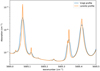 |
Fig. A.1 Absorption spectrum assuming a Voigt or a Lorentz profile at the same resolution (0.001 cm−1) with P=1000 Pa and T=300 K. As the wings of the absorption lines do not follow a Voigt profile, we only considered the centre of the lines up to 25 cm−1here. |
A.1.2 Continua
In this work, for both radiative transfer methods, we used the MT_CKD formalism with a cut-off of the centre of the water ab- sorption lines at 25 cm−1 and a removed plinth. A continuum is added to take into account the far-wing absorption. Yang et al. (2016) showed through a model inter-comparison that a source of difference of the OLR values comes from the radiative transfer, and more particularly from the continua used. It is interesting to note that a part of the difference between our results and those of Kopparapu et al. (2013) is due to the choice of the H2O continuum database. They used BPS (Paynter & Ramaswamy 2011), while we used MT_CKD.
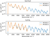 |
Fig. A.2 Comparison of H2O-H2O and H2O-N2 continua from MT_CKD2.5 and 3.2 databases. Here, the y-axis is in logscale. |
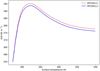 |
Fig. A.3 OLR values as a function of the surface temperature for P |

A spectral comparison of the water continua used in this work is provided in Fig. A.2. The main difference between MT_CKD2.5 and MT_CKD3.2 comes from the wavelength definition domain. The MT_CKD2.5 continuum is defined between 0 cm−1 and 10000 cm−1, while the MT_CKD3.2 continuum is defined up to 20000 cm−1, as shown in Fig. A.2. Nevertheless, as the vast majority of the absorption of the water is between 0 cm−1 and 5000 cm−1, the difference in the OLR value is at most 1.5 W.m2 (Fig. A.3). We used the MT_CKD3.2 continua in PyRADS-Conv1D to increase our accuracy but also for computational reasons. If the continnum is not defined for a spectral range, it becomes necessary to compute the absorption lines up to a few hundreds of cm−1 to accurately represent the spectrum. This increases the computation time drastically. The N2 -N2 continuum from the HITRAN CIA database even has a negligible impact on the OLR (less than 1 W/m2) at a low temperaturefor  =10 bar when the nitrogen pressure is largely dominating the vapour pressure.
Overview of sensitivity tests performed with the impact on the computed OLR value. The Original param. column indicates the parametrisation used in the considered model, and the Tested param. column shows the tested parametrisation. The OLR difference between original and modified parametrisations is indicated in the OLR difference column.
A.1.3 Water isotopes
There is no real consensus to include (or not include) the absorption lines of the secondary water isotopes in the radiative transfer computation. Similarly, there is no consensus as to what their abundances may be in other worlds. To have an idea of the potential impact of water isotopes on the OLR computation for an Earth-like planet, we considered different case studies with different isotopes abundances: Iso1 (terrestrial abundances, De Biévre et al. 1984; Gordon et al. 2017), Iso2 (all the secondary isotopes are two times more abundant), Iso10 (all the secondary isotopes are ten times more abundant), Iso100 (all the secondary isotopes are 100 times more abundant), Iso2HD (the HD16O, HD17O and HD18O isotopes are two times more abundant), Iso10HD (the HD16O, HD17O and HD18O isotopes are ten times more abundant), Iso100HD (the HD16O, HD17O and HD18O isotopes are 100 times more abundant).
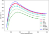 |
Fig. A.4 OLR values as a function of the surface temperature for P |

For each case study, we adjusted the abundance of the main isotope to keep a total abundance equal to unity (see Table A.2). Figure A.4 shows that secondary isotopes slightly reduce the height of the overshoot even at a terrestrial abundance (Iso1), but this difference is lower than 2 W.m2. At higher abundances (Iso2, Iso10, Iso100), the strong absorption of the secondary isotopes reduces the OLR value over the entire studied temperature range. The tendency is the same when only increasing abundances of the HDXO isotopes (Iso2HD, Iso10HD, Iso100HD) Nevertheless, Fig. A.4 shows that increasing the abundance of all the secondary isotopes more efficiently reduces OLR than only increasing HDXO abundances (Iso100 and Iso100HD).
A.1.4 CO2
The typical atmospheric compositions of moderately irradiated rocky exoplanets is currently unknown. A common solution to fill this gap is to consider an Earth-like atmosphere. Therefore, several studies added a few parts-per-million of CO2 in the atmosphericcomposition, such as Kopparapu et al. (2014), who added 350 ppm (Ravi K. Kopparapu, priv. comm.). Such an amount of CO2 can stronglychange the OLR values but also the shape of the OLR curve (Fig. A.5). The difference induced by CO2 is higher at low temperatures, where water is not the dominant gas. In other words, for such low temperatures the absorption due to CO2 is non-negligible. At high temperatures, the absorption due to water is high enough to overlap the CO2 absorption. For this reason, if there is CO2 in the simulated atmosphere, it is important to consider it in the analysis to avoid incorrect conclusions.
In this work, as we explored the effects of nitrogen, we considered an H2O + N2 atmosphere without CO2. A few papers (e.g. Ramirez et al. 2014; Popp et al. 2016) discuss the effect of CO2 on the onset of the runaway greenhouse in more detail. In Fig. A.5, as the CO2 quantity is a percentage of the N2 pressure (we used 376 ppm of CO2, as Leconte et al. 2013), the amount of CO2 increases when increasing the N2 pressure. This is the reason why the difference between simulations with and without CO2 is stronger at high N2 pressure. The strong greenhouse power of the CO2 also strongly reduces the height of the overshoot. Finally, CO2 absorption explains a large part of the gap between the results of Kopparapu et al. (2014) and those of other.
Overview of the isotope abundances per isotope (Isotopes) for the different case studies. The Iso1 case study corresponds to terrestrial abundances (Terr. abun.) while, for the Iso2, Iso10, and Iso100 cases, secondary isotope abundances are multiplied by 2, 10, and 100. For the Iso2HD, Iso10HD, and Iso100HD cases we increase only the abundance of HDX O isotopes by multiplying them by a factor of 2, 10, or 100.
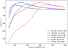 |
Fig. A.5 OLR values as a function of the surface temperature with and without CO2 computed with Exo_k. The full lines are the reference OLR curves proposed in Fig. 3 using Exo_k, and the dotted lines include 376 ppm of CO2 in the radiative transfer computation. |
A.1.5 Two-stream approximation
All the radiative transfer models used here employ a two-stream approximation in the infrared where the radiative transport inthe atmosphere is described by an upward and a downward flux (Meador & Weaver 1980; in fact, as we are focused on the thermal emission in a non-scattering atmosphere, we are only really dealing with one stream).
Since the seminal work of Toon et al. (1989), it is known that, while this approach is numerically efficient, the assumptions made (e.g. the two-stream coefficients used) need to be adapted to the problem at hand to ensure accuracy. For example, as can be seen in Fig. A.6, the classical hemispheric mean approximation (where the intensity is considered constant over each hemisphere)systematically underestimates the outgoing emitted flux compared to a proper integration over the cosine of the zenith angle (μ). This is due to the fact that for a given specific intensity (considered independent of the azimuth angle), I(μ), the integral for the upward flux,
 (A.1)
(A.1)
gives more weight to the rays close to the vertical. Because these rays probe deeper, they have a higher than average intensity (see Fig. A.6, where we show πI(μ) to use the same scale as the flux). From this figure, we see that the total flux would be better approximated by πI(μ ~ 0.6); thus, one might be tempted to use the classical quadrature method and choose  as the quadrature point. As pointed out by Toon et al. (1989), however, this approach leads to a well-known unphysical emissivity that is highly undesirable if one wants to conserve energy.
To avoid having to use an expensive angular integration while preserving an accurate and physical solution, the Exo_k-RT method (Table 1) uses the following approximation in the infrared, which is a variation on the hemispheric approximation. Following notations from Toon et al. (1989), the equation for the upward flux (and similarly for the downward flux, F−) writes
 (A.2)
(A.2)
where γ1 = 2 − ω0(1 + g) and γ2 = ω0(1 − g), ω0 and g are the single scattering albedo and asymmetry factor of the medium, and B is the Planck function. The difference with the classical hemispheric approximation is the factor ϵ that accounts forthe fact that, when assuming the hemi-isotropy of the intensity, choosing an effective optical depth (dτ∕ϵ) that is different from the vertical one does not introduce a greater level of approximation.
Interestingly, choosing an effective zenith angle whose cosine is  and defining
  7, Eq. (A.2) rewrites
 (A.3)
(A.3)
By comparison with Table 1 of Toon et al. (1989), one can directly see that this assumption is completely equivalent to the quadrature approximation where an arbitrary quadrature point  is chosen instead of the Gauss-Legendre choice (1/
 ), except for the change to the source term. This change is what makes our approximation retain the physical consistency of the hemispheric mean approach as F+ → πB in an opaque, non-scattering medium, whatever
  we choose.
Our modified hemispheric-mean approximation, which is the default method in Exo_k, thus combines the energy-conserving feature of the classical hemispheric-mean with the flexibility of choosing the best effective zenith angle for a given problem. In practice it is easy to adapt any numerical implementation of the classical two-stream approach to solve this system: i) use the γ coefficients from Eq. (A.3) and ii) change the 2πμ1 coefficient in Eq. (27) of Toon et al. (1989) into π to enforce energy conservation.
In the context of a non-scattering atmosphere, it is easy to show that our modified hemispheric-mean approximation is equivalent to computing the intensity for a given  and assuming
  . As can be seen in Fig. A.6 and is discussed above,
  yields a less than 1 W.m−2 difference over the whole range of atmospheres modelled here. However, we highlight that care should be given to the radiative transfer method used when comparing model results as different methods can lead to differences of ~ 6 W/m2. These differences are visible between kcm1d (which uses the classical hemispheric mean approximation) and PyRADS (which assumes
  with
with  ) in Fig. 1.
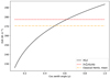 |
Fig. A.6 Variation of OLR with respect to the effective zenith angle used to compute the upward intensity (solid curve). The dashed curve shows the OLR computed by properly integrating the intensity over all zenith angles. The horizontal dash-dot curve shows the result of the classical hemispheric mean approximation (Toon et al. 1989), which systematically underestimates the flux by
~6 W.m−2. The atmosphere model used has Tsurf=500 K and P |

A.1.6 Convection scheme
The two convection schemes used in this work and presented in Sect. 2.1 are based on the two main adiabatic lapse rates available in the literature. In Appendix B, we show that the difference between them comes from the definition of the entropy of the condensable gas. As explained in Sect. 2.1, we used the Conv_K88 scheme as reference because it is based on look-up tables, which is more accurate than the perfect gas laws used inthe Conv_D16 scheme. It is interesting to quantify the uncertainty bewteen OLR curves computed using one scheme or the other. We modified PyRADS-Conv1D to use the Conv_K88 of the Conv_D16 scheme and we obtained the curves presented in Fig. A.7. We show that the difference is smaller than 5 W.m2. We also notice that the Conv_D16 scheme systematically underestimates the OLR, probably mainly by overestimating the water content.
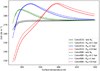 |
Fig. A.7 OLR values as a function of the surface temperature for different nitrogen pressures assuming the Conv_K88 or the Conv_D16 scheme using PyRADS-Conv1D. |
A.2 Sensitivity studies on numerical setup
The second set of sensitivity tests is focused on numerical parametrisations.
A.2.1 Vertical grid resolution
Aside from using two different adiabats, the convective schemes used in this work assume two different definitions of the vertical grid. The Conv_D16 scheme provides a logarithmic distribution of the levels with a fixed difference between the surface pressure and pressure at the top of the atmosphere, while the Conv_K88 scheme adapts the height of the levels relatively to the amount of water from the surface up to 0.1 Pa (Fig. A.8). In other words, in the Conv_K88 scheme the wet atmospheric levels near the surface are thinner than the drier ones at the top of the atmosphere. The aim is to increase the vertical resolution of the ’radiatively active’ part of the atmosphere. The number of vertical levels required to compute an accurate value of the OLR does not depend on the nitrogen pressure or on the surface pressure, but this number is higher than for the Conv_D16 scheme. Consequently, using the Conv_K88 scheme is more accurate even if the computation time is more expensive. For this reason, we used it in PyRADS-Conv1D. A convergence curve of the OLR relative to the number of vertical levels highlights that 200 levels are needed for the Conv_K88 scheme to keep an error smaller than 1W/m2 compared tothe converged OLR value. We assumed a stratospheric temperature equal to 200 K according to Kasting (1988). That work showed that a value lower than 250 K does not influence the OLR because for such low stratospheric temperatures the vapour pressure is radiatively negligible in the upper layers of the atmosphere (by assuming a pseudo-adiabatic approximation).
In the Conv_D16 scheme, the vertical grid does not depend only on the number of levels but also on the difference inpressure between the top and the bottom of the atmosphere. This induces a dependency on the number of levels on the surface temperature as shown in Table A.3. Indeed, because of the pseudo-adiabatic approximation the total surface pressure increases strongly between 280 K and 500 K (≈1 bar to ≈26 bar if P =1 bar), and the difference between pressures at the top and at the bottom of the atmosphere may be high to accurately represent the whole atmosphere. Moreover, increasing the nitrogen pressure reduces the height of the radiatively active part of the atmosphere by drying it up; thus, the required number of levels increases. We also observed that using a stratospheric temperature equal to 150 K (and not 200 K as in the Conv_K88 scheme) allows us to slightly reduce the required number of levels. Finally, according to Table A.3, in the Conv_D16 scheme we assume 100 vertical levels and a difference between the pressure at the bottom and at the top of the atmosphere equal to 106 Pa. This setup provides a good compromise between accuracy and computation time with an error at most equal to 1 W/m2 compared to the converged value.
Overview of the number of atmospheric levels needed in the Conv_D16 scheme relatively to the nitrogen pressure, the surface temperature (Tsurf), the stratospheric temperature (Tstrat), and the difference between the pressure at the bottom and at the top of the atmosphere (Pres. diff.).
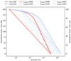 |
Fig. A.8 Comparison of pressure distribution over the vertical grid of the model for the Conv_K88 and the Conv_D16 methods. Here, P |

A.2.2 Spectral resolution
For the line-by-line method, as we assume a Lorentz profile for the absorption lines, the spectral resolution needs to be high enough to accurately reproduce the real spectrum. The line-by-line method needs a minimal spectral resolution of 0.01 cm−1 to give an accurate value of the OLR (Fig. A.9) as shown by Koll & Cronin (2018). The absorption lines are not exactly resolved, as is visible in Fig. A.10, but the cumulative error on the entire spectrum is negligible. Producing acorrelated-k table requires high-resolution spectra; therefore, we used a spectral resolution of 0.001 cm−1, which is able to resolve each absorption line. Fig. A.10 shows that by increasing the pressure and the temperature, the width of the line becomes larger; thus, a lower resolution is sufficient. Nevertheless, in the highest atmospheric levels the pressureis low, and a high spectral resolution is always required.
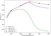 |
Fig. A.9 OLR values as a function of the surface temperature for different spectral resolution with P |

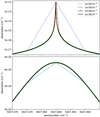 |
Fig. A.10 Absorption line at 5027.460050 cm−1 for different spectral resolutions and using a Lorentz profile. The top panel is the absorption for P=6 Pa and T=220 K, and the bottom panel is the absorption for P=3500 Pa and T=300 K. |
A.2.3 Correlated-k-mixing ratio grid
Because of the non-usual transition between an N2 -dominated and an H2O atmosphere, we tested the resolution of the volume-mixing ratio (vmr) grid of the correlated-k table. The original resolution of the vmr grid (Q = {1e−6, 1e−5, 1e−4, 1e−3, 1e−2, 1e−1, 1}) was increased to Q = {1e−6, 1e−5, 1e−4, 1e−3, 1e−2, 5e−2, 1e−1, 5e−1, 1}, but it does not significantly change the OLR values.
A.2.4 Correlated-k-interpolation scheme
Correlated-k tables contain absorption spectra for given pressure, temperature, and vmr grids. To be able to compute the absorption of each atmospheric level, the models need to interpolate these tables on different pressure, temperature, and vmr values. Because of the wide diversity of interpolation schemes, we do not describe them in detail. However, by using two different schemes (from two different models), we caveat that a part of the differences highlighted in Fig. 1 can come from the choice of the correlated-k-interpolation scheme.
The two correlated-k radiative transfer models we used in this work (Exo_k and kcm1d in Table 1) have different interpolation schemes and produce different OLR curves for the same correlated-k table. Nevertheless, this difference is smaller than 3 W.m2. We were able to reproduce OLR curves from kcm1d with a modified version of Exo_k that uses the same interpolation scheme as kcm1d, with an error lower than 1 W.m2. This proves that the only difference in Fig. A.11 comes from the interpolation scheme. As kcm1d is derived from the LMD-Generic model, it inherits an interpolation scheme optimised for such 3D models; thus, this difference of 3 W.m2 is a second-order error regarding other uncertainties of GCMs.
Although the detail of the interpolation of Exo_k and kcm1d are different, the global scheme is the same. The absorption spectrum (K) is interpolated on the pressure (P), temperature (T), and vmr (x) as follows:
![Mathematical equation: \[ \mathrm{\ln K=fct(\ln P, T, \ln x).} \]](/articles/aa/full_html/2022/02/aa42286-21/aa42286-21-eq30.png)
This global scheme provides the most accurate interpolated spectra, which makes sense regarding the logarithmic distribution of the pressure and vmr grids of the correlated-k tables.
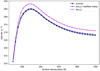 |
Fig. A.11 OLR as a function of the surface temperature for different interpolation schemes: kcm1d (black line) and Exo_k(magenta line). The blue line corresponds to Exo_k using the kcm1d interpolation scheme. Here, P |

Appendix B Adiabatic lapse rate formulations
One-dimensional radiative-convective climate models usually use a pseudo-adiabatic lapse rate (also referred to as adiabat) to compute the temperature profile of the atmosphere. There are two widely used formulations of this adiabat in the literature for a moist atmosphere. The first one is proposed by Kasting (1988) based on Ingersoll (1969):
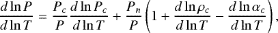 (B.1)
(B.1)
with
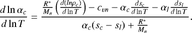 (B.2)
(B.2)
The second one is proposed by Ding & Pierrehumbert (2016) based on the dry adiabat of Pierrehumbert (2010):
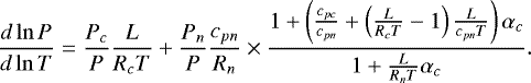 (B.3)
(B.3)
Both moist lapse rates presented above are valid for a non-dilute atmosphere (i.e. for an atmosphere where water is a trace gas). Leconte et al. (2013, 2017) proposed a third formulation equivalent - but not strictly equal - to Ding & Pierrehumbert (2016) (see Eq. (B.4)). Nevertheless, Leconte et al. (2017) highlighted an interesting molecular mass gradient effect.
Through a few mathematical reformulations of the adiabat proposed by Leconte et al. (2013), we obtain the following equation, which is strictly equal to Eq. (B.3) under the pseudo-adiabatic approximation (i.e. αl = 0):
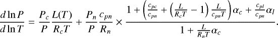 (B.4)
(B.4)
Indices of variables in the Eqs. (B.3), (B.1), (B.2), and (B.4) indicate what gas is considered: c for the condensable gas, n for the non-condensable gas, and l for the condensed gas. Here, P is the pressure, T the temperature, M the molecular weight, ρ the density, R* the perfect gas constant, R the specific gas constant, αi = mi∕mn the mass-mixing ratio per unit of non-condensable gas (mn) for the species i, L the latent heat, and cp the heat capacity.
These equations are different but can be equalised through three simple equations. The main difference between Eqs. (B.3) and (B.1) comes from the initial definition of the entropy. Indeed, Eq. (B.3 defines the entropy of the condensable gas as a perfect gas entropy. Equation (B.1) does not state the entropy of the condensable gas. Therefore, it is possible to use values from experiments for the condensable entropy to reduce inaccurate results at high temperatures (i.e. near the critical point). In both cases, the total gas pressure is defined using the perfect gas law.
B.1 Development of the adiabatic lapse rate of Ding & Pierrehumbert (2016)
We start with the definition of the total heat budget per unit of mass δQm. Here, we consider a volume per unit of mass (dV∕m):
 (B.5)
(B.5)
where 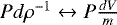 and
and  . Using Eq. (B.5), we define the total heat budget δQ of a gas mixture (Pierrehumbert 2010):
![Mathematical equation: \[ \delta Q=(m_n+m_c)\delta Q_m=m_nc_{pn}dT-\frac{m_n}{\rho_n}dP_n+m_cc_{pc}dT-\frac{m_c}{\rho_c}dP_c+Ldm_c, \]](/articles/aa/full_html/2022/02/aa42286-21/aa42286-21-eq38.png)
where δQ is the total heat budget and δQm is the total heat budget per unit of mass. We consider a pseudo-adiabatic system, and thus all the condensation is immediatelyremoved by precipitation. In other words, the pressure of the condensable gas is equal to the saturation pressure.
By dividing the previous equation by the mass of the non-condensable gas (mn) we obtain the total heat budget per unit of non-condensable gas:
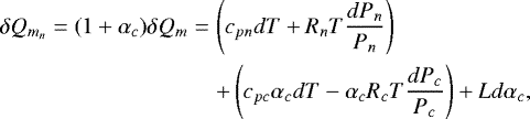 (B.6)
(B.6)
where αc = mc∕mn. By dividing the previous equation by the temperature then by rewriting it, we obtain
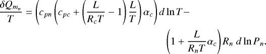 (B.7)
(B.7)
By definition of an adiabatic (or pseudo-adiabatic) transformation, δQ = 0. Therefore, it is possible to define the dry adiabatic lapse rate (Pierrehumbert 2010):
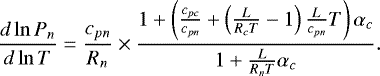 (B.8)
(B.8)
By assuming that the total pressure is the sum of both condensable and non-condensable pressures, we obtain
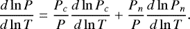 (B.9)
(B.9)
Then, by using Eqs. (B.10) and (B.11) and the equation of Clausius-Clapeyron (Eq. (B.12)),
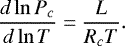 (B.10)
We obtain the moist adiabatic lapse rate proposed by Ding & Pierrehumbert (2016) (Eq. (B.3). We assume that cp does not depend on temperature, but this assumption becomes false near the critical point.
B.2 Development of the adiabatic lapse rate of Kasting (1988)
The moist adiabatic lapse rate proposed by Kasting (1988) uses equations from Ingersoll (1969). First, Ingersoll (1969) assumed the entropy of an adiabaticsystem S, per unit of mass of non-condensable gas:
 (B.11)
where sn, sc, and sl are the entropies of the non-condensable, the condensable, and the liquid part, and  . Near the critical point, it may not be valid to treat each constituent separately. By rewriting Eq. (B.13), we obtain
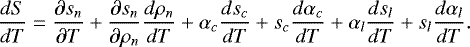 (B.12)
The law of mass conservation during an adiabatic expansion provides the following equality:
![Mathematical equation: \[ \frac{d\alpha_l}{dT}=-\frac{d\alpha_c}{dT,} \]](/articles/aa/full_html/2022/02/aa42286-21/aa42286-21-eq47.png)
and, using  ,
,
![Mathematical equation: \[ \frac{d\rho_n}{dT} = \frac{1}{\alpha_c}\frac{d\rho_c}{dT}-\frac{\rho_c}{\alpha_c^2}\frac{d\alpha_c}{dT.} \]](/articles/aa/full_html/2022/02/aa42286-21/aa42286-21-eq49.png)
Thanks to these equalities, we can rewrite Eq. (B.14):
![Mathematical equation: \[ \frac{dS}{dT}=\frac{\partial s_n}{\partial T}+\frac{1}{\alpha_c} \frac{\partial s_n}{\partial \rho_n}\left(\frac{d\rho_c}{dT}-\frac{\rho_c}{\alpha_c}\frac{d\alpha_c}{dT}\right) +\alpha_c\frac{ds_c}{dT}+\alpha_l\frac{ds_l}{dT}+(s_c-s_l)\frac{d\alpha_c}{dT.} \]](/articles/aa/full_html/2022/02/aa42286-21/aa42286-21-eq50.png)
If the non condensable gas behaves as an ideal gas, we can assume  and
and 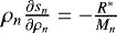 ; thus,
 (B.13)
From Eq. (B.15) by assuming the adiabatic hypothesis (dS = 0), we obtain Eq. (B.16) (Ingersoll 1969) and Eq. (B.17) (Kasting 1988):
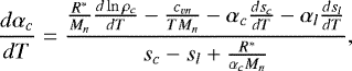 (B.14)
 (B.15)
As in Kasting (1988), from now we assume a pseudo-adiabatic expansion; hence, αl = 0. By assuming that the total pressure is the sum of both condensable and non-condensable pressures, and using the perfect gas law, we obtain
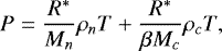 (B.16)
where β = β(ρc, T) is a parameter that expresses the degree to which the condensable gas departs from ideality. By rewriting Eq. (B.18) and using Eq. (B.17), we obtain the adiabatic lapse rate proposed by Kasting (1988):
 (B.17)
Here, the entropy of the condensable part (sc) is explicitly defined in the equation. In the Conv_K88 scheme, which uses Kasting (1988) equations, we compute the water entropy thanks to experimental look-up tables (Haar et al. 1984).
B.3 Equalisation of the adiabatic lapse rates
The two formulations of the adiabatic lapse rate (Eqs. (B.3) and (B.1)) can be equalised assuming the following assumptions:
- A.
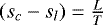
- B.
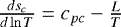
- C.
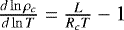
By definition, equality A is always verified and corresponds to the entropy of phase change. Equalities B and C are only verified if we use the equation of Clausius-Clapeyron (Eq. B.12) to link vapour pressure, temperature, and latent heat.
We show here that the main difference between adiabatic lapse rates from Kasting (1988) and Ding & Pierrehumbert (2016) comes from the definition of the entropy of the condensable gas. Indeed, Eq. (B.3) (Ding & Pierrehumbert 2016) implicitly uses the definition of the entropy of a perfect gas (Pierrehumbert 2010), which becomes incorrect at high temperatures (i.e. near the critical point). The second difference is the use of the Clausius-Clapeyron equation (Eq. (B.12)), which is an approximation of the more general Clausius equation. This Clausius-Clapeyron equation is only valid for a perfect gas far from the critical point. For these reasons, we choose to use the Conv_K88 method based on the moist adiabatic lapse rate from Kasting (1988) for PyRADS-Conv1D, used as a reference in this paper.
References
- Amundsen, D. S., Tremblin, P., Manners, J., Baraffe, I., & Mayne, N. J. 2017, A&A, 598, A97 [NASA ADS] [CrossRef] [EDP Sciences] [Google Scholar]
- Boukrouche, R., Lichtenberg, T., & Pierrehumbert, R. T. 2021, ApJ, 919, 130 [NASA ADS] [CrossRef] [Google Scholar]
- De Biévre, P., Gallet, M., Holden, N. E., & Barnes, I. L. 1984, J. Phys. Chem. Ref. Data, 13, 809 [CrossRef] [Google Scholar]
- Ding, F., & Pierrehumbert, R. T. 2016, ApJ, 822, 24 [CrossRef] [Google Scholar]
- Fauchez, T. J., Turbet, M., Sergeev, D. E., et al. 2021, PSJ, 2, 106 [NASA ADS] [Google Scholar]
- Fu, Q., & Liou, K. N. 1992, J. Atmos. Sci., 49, 2139 [Google Scholar]
- Goldblatt, C., & Watson, A. J. 2012, Philos. Trans. R. Soc. A: Math. Phys. Eng. Sci., 370, 4197 [NASA ADS] [CrossRef] [Google Scholar]
- Goldblatt, C., Robinson, T. D., Zahnle, K. J., & Crisp, D. 2013, Nat. Geosci., 6, 661 [NASA ADS] [CrossRef] [Google Scholar]
- Gordon, I. E., Rothman, L. S., Hill, C., et al. 2017, J. Quant. Spectr. Rad. Transfer, 203, 3 [NASA ADS] [CrossRef] [Google Scholar]
- Haar, L., Gallagher, J. S., & Kell, G. S. 1984, NBS/NRC Steam Tables: Thermodynamic and Transport Properties and Computer Programs for Vapor and Liquid States of Water in SI Units (Washington (D.C.): Hemisphere) [Google Scholar]
- Ingersoll, A. P. 1969 J. Atm. Sci., 26, 1191 [NASA ADS] [CrossRef] [Google Scholar]
- Karman, T., Gordon, I. E., van der Avoird, A., et al. 2019, Icarus, 328, 160 [Google Scholar]
- Kasting, J. F. 1988, Icarus, 74, 472 [NASA ADS] [CrossRef] [Google Scholar]
- Kasting, J. F., Whitmire, D. P., & Reynolds, R. T. 1993, Icarus, 101, 108 [Google Scholar]
- Koll, D. D. B., & Cronin, T. W. 2018, Proc. Natl. Acad. Sci. U.S.A., 115, 10293 [CrossRef] [Google Scholar]
- Koll, D. D. B., & Cronin, T. W. 2019, ApJ, 881, 120 [Google Scholar]
- Komabayasi, M. 1967, J. Meteorol. Soc. Jpn. Ser. II, 45, 137 [NASA ADS] [CrossRef] [Google Scholar]
- Kopparapu, R. k., Ramirez, R., Kasting, J. F., et al. 2013, ApJ, 765, 131 [NASA ADS] [CrossRef] [Google Scholar]
- Kopparapu, R. k., Ramirez, R. M., SchottelKotte, J., et al. 2014, ApJ, 787, L29 [NASA ADS] [CrossRef] [Google Scholar]
- Leconte, J. 2021, A&A, 645, A20 [NASA ADS] [CrossRef] [EDP Sciences] [Google Scholar]
- Leconte, J., Forget, F., Charnay, B., Wordsworth, R., & Pottier, A. 2013, Nature, 504, 268 [Google Scholar]
- Leconte, J., Selsis, F., Hersant, F., & Guillot, T. 2017, A&A, 598, A98 [NASA ADS] [CrossRef] [EDP Sciences] [Google Scholar]
- Marcq, E., Salvador, A., Massol, H., & Davaille, A. 2017, J. Geophys. Res. (Planets), 122, 1539 [NASA ADS] [CrossRef] [Google Scholar]
- Meador, W. E., & Weaver, W. R. 1980, J. Atmos. Sci., 37, 630 [NASA ADS] [CrossRef] [Google Scholar]
- Meadows, V. S., & Crisp, D. 1996, J. Geophys. Res., 101, 4595 [NASA ADS] [CrossRef] [Google Scholar]
- Mlawer, E. J., Payne, V. H., Moncet, J.-L., et al. 2012, Philos. Trans. R. Soc. Lond. A, 370, 2520 [NASA ADS] [Google Scholar]
- Nakajima, S., Hayashi, Y.-Y., & Abe, Y. 1992, J. Atmos. Sci., 49, 2256 [NASA ADS] [CrossRef] [Google Scholar]
- Paynter, D. J., & Ramaswamy, V. 2011, J. Geophys. Res. (Atmospheres), 116, D20302 [NASA ADS] [CrossRef] [Google Scholar]
- Pierrehumbert, R. T. 2010, Principles of Planetary Climate (Cambridge; New York: Cambridge University Press), oCLC: ocn601113992 [CrossRef] [Google Scholar]
- Popp, M., Schmidt, H., & Marotzke, J. 2016, Nat. Commun., 7, 10627 [NASA ADS] [CrossRef] [Google Scholar]
- Ramirez, R. M. 2020, MNRAS, 494, 259 [NASA ADS] [CrossRef] [Google Scholar]
- Ramirez, R. M., Kopparapu, R. K., Lindner, V., & Kasting, J. F. 2014, Astrobiology, 14, 714 [NASA ADS] [CrossRef] [Google Scholar]
- Simpson, G. C. 1929, Q. J. R. Meteorol. Soc., 55, 73 [Google Scholar]
- Toon, O. B., McKay, C. P., Ackerman, T. P., & Santhanam, K. 1989, J. Geophys. Res., 94, 16287 [Google Scholar]
- Turbet, M., Ehrenreich, D., Lovis, C., Bolmont, E., & Fauchez, T. 2019, A&A, 628, A12 [NASA ADS] [CrossRef] [EDP Sciences] [Google Scholar]
- Turbet, M., Bolmont, E., Chaverot, G., et al. 2021, Nature, 598, 276 [CrossRef] [Google Scholar]
- Wolf, E. T. 2017, ApJ, 839, L1 [Google Scholar]
- Yang, J., Cowan, N. B., & Abbot, D. S. 2013, ApJ, 771, L45 [Google Scholar]
- Yang, J., Leconte, J., Wolf, E. T., et al. 2016, ApJ, 826, 222 [NASA ADS] [CrossRef] [Google Scholar]
- Yang, J., Leconte, J., Wolf, E. T., et al. 2019, ApJ, 875, 46 [NASA ADS] [CrossRef] [Google Scholar]
- Zhang, Y., & Yang, J. 2020, ApJ, 901, L36 [NASA ADS] [CrossRef] [Google Scholar]
For each spectral line ν, the MT_CKD continuum formalism assumes a constant absorption value between ν - 25 cm−1 and ν + 25 cm−1 equal to the absorption at ν ± 25 cm−1. Consequently this ‘plinth’ needs to be removed in the line centre calculation.
The factor of 2 comes from the fact that the hemispheric-mean approximation can be seen as looking at a ray with
 , so that ϵ can be seen as a correction factor accounting for the departure from the hemispheric-mean effective zenith angle.
All Tables
Molecular weight (M), heat capacity (cp), and molecular heat capacity (cp,molec) for different background gases (Gas), where cp,molec = cp × M.
Overview of sensitivity tests performed with the impact on the computed OLR value. The Original param. column indicates the parametrisation used in the considered model, and the Tested param. column shows the tested parametrisation. The OLR difference between original and modified parametrisations is indicated in the OLR difference column.
Overview of the isotope abundances per isotope (Isotopes) for the different case studies. The Iso1 case study corresponds to terrestrial abundances (Terr. abun.) while, for the Iso2, Iso10, and Iso100 cases, secondary isotope abundances are multiplied by 2, 10, and 100. For the Iso2HD, Iso10HD, and Iso100HD cases we increase only the abundance of HDX O isotopes by multiplying them by a factor of 2, 10, or 100.
Overview of the number of atmospheric levels needed in the Conv_D16 scheme relatively to the nitrogen pressure, the surface temperature (Tsurf), the stratospheric temperature (Tstrat), and the difference between the pressure at the bottom and at the top of the atmosphere (Pres. diff.).
All Figures
|
Fig. 1 OLR as a function of surface temperature for different N2 partial pressures ( |
| In the text | |
|
Fig. 2 Comparison between Conv_K88 (full lines) and Conv_D16 (dotted lines) convection schemes for different surface temperatures. The top panel represents the temperature profiles, and the bottom panel represents the volume-mixing ratio of the water for different surface temperatures. Here,
|
| In the text | |
|
Fig. 3 OLR as a function of the surface temperature (top panel) or as a function of the nitrogen pressure (bottom panel). The top panel represents the OLR curve for different N2 pressures (black: |
| In the text | |
|
Fig. 4 OLR and corresponding atmospheric water content as a function of the surface temperature. The top panel is the OLR as a function of the surface temperature for different nitrogen pressure, computed with PyRADS-Conv1D. The three bottom panels represent the size of the atmosphere (up to 0.1 Pa)for different nitrogen pressures where the colour bar indicates the water-volume-mixing ratio ( |
| In the text | |
|
Fig. 5 OLR as a function of the volume-mixing ratio for different nitrogen surface pressures using Exo_k. The volume-mixing ratio (vmr) values are given at the top of the atmosphere (top panel), at 0.01 bar (middle panel), and at 0.1 bar (bottom panel) of total pressure. The black cross represent the Simpson-Nakajima limit for a pure vapour atmosphere,and the vertical dashed lines approximately delimit the range of vmr values for which there is a transition of dominantspecies. |
| In the text | |
|
Fig. 6 OLR as a function of the temperature for |
| In the text | |
|
Fig. 7 Temperature profiles computed with the Conv_K88 scheme for different surface temperatures with
|
| In the text | |
|
Fig. 8 OLR as a function of the surface temperature by only using the physical properties of other gases in the convective scheme calculation (top panel), in the radiative transfer calculation only (middle panel) and in both of them (bottom panel). The full blue line corresponds to the curve presented in the top panel of Fig. 3 with the true value of the nitrogen molecular weight. The dotted lines correspond to Mn and cp values of other gases (see Table 2). Here, we used the Conv_D16 scheme and the Exo_k-RT radiative transfer method assuming 1 bar of background gas. |
| In the text | |
|
Fig. A.1 Absorption spectrum assuming a Voigt or a Lorentz profile at the same resolution (0.001 cm−1) with P=1000 Pa and T=300 K. As the wings of the absorption lines do not follow a Voigt profile, we only considered the centre of the lines up to 25 cm−1here. |
| In the text | |
|
Fig. A.2 Comparison of H2O-H2O and H2O-N2 continua from MT_CKD2.5 and 3.2 databases. Here, the y-axis is in logscale. |
| In the text | |
|
Fig. A.3 OLR values as a function of the surface temperature for P |
| In the text | |
|
Fig. A.4 OLR values as a function of the surface temperature for P |
| In the text | |
|
Fig. A.5 OLR values as a function of the surface temperature with and without CO2 computed with Exo_k. The full lines are the reference OLR curves proposed in Fig. 3 using Exo_k, and the dotted lines include 376 ppm of CO2 in the radiative transfer computation. |
| In the text | |
|
Fig. A.6 Variation of OLR with respect to the effective zenith angle used to compute the upward intensity (solid curve). The dashed curve shows the OLR computed by properly integrating the intensity over all zenith angles. The horizontal dash-dot curve shows the result of the classical hemispheric mean approximation (Toon et al. 1989), which systematically underestimates the flux by
~6 W.m−2. The atmosphere model used has Tsurf=500 K and P |
| In the text | |
|
Fig. A.7 OLR values as a function of the surface temperature for different nitrogen pressures assuming the Conv_K88 or the Conv_D16 scheme using PyRADS-Conv1D. |
| In the text | |
|
Fig. A.8 Comparison of pressure distribution over the vertical grid of the model for the Conv_K88 and the Conv_D16 methods. Here, P |
| In the text | |
|
Fig. A.9 OLR values as a function of the surface temperature for different spectral resolution with P |
| In the text | |
|
Fig. A.10 Absorption line at 5027.460050 cm−1 for different spectral resolutions and using a Lorentz profile. The top panel is the absorption for P=6 Pa and T=220 K, and the bottom panel is the absorption for P=3500 Pa and T=300 K. |
| In the text | |
|
Fig. A.11 OLR as a function of the surface temperature for different interpolation schemes: kcm1d (black line) and Exo_k(magenta line). The blue line corresponds to Exo_k using the kcm1d interpolation scheme. Here, P |
| In the text | |
Current usage metrics show cumulative count of Article Views (full-text article views including HTML views, PDF and ePub downloads, according to the available data) and Abstracts Views on Vision4Press platform.
Data correspond to usage on the plateform after 2015. The current usage metrics is available 48-96 hours after online publication and is updated daily on week days.
Initial download of the metrics may take a while.