| Issue |
A&A
Volume 658, February 2022
|
|
|---|---|---|
| Article Number | A23 | |
| Number of page(s) | 12 | |
| Section | The Sun and the Heliosphere | |
| DOI | https://doi.org/10.1051/0004-6361/202142002 | |
| Published online | 27 January 2022 | |
Energetic proton back-precipitation onto the solar atmosphere in relation to long-duration gamma-ray flares
1
Jeremiah Horrocks Institute, University of Central Lancashire, Preston PR1 2HE, UK
e-mail: This email address is being protected from spambots. You need JavaScript enabled to view it.
2
Heliophysics Division, NASA Goddard Space Flight Center, Greenbelt, MD, USA
3
Department of Physics, Catholic University of America, Washington, DC, USA
4
Department of Physics and Astronomy, University of New Hampshire, Durham, NH, USA
Received:
11
August
2021
Accepted:
6
November
2021
Abstract
Context. Gamma-ray emission during long-duration gamma-ray flare (LDGRF) events is thought to be caused mainly by > 300 MeV protons interacting with the ambient plasma at or near the photosphere. Prolonged periods of the gamma-ray emission have prompted the suggestion that the source of the energetic protons is acceleration at a coronal mass ejection (CME)-driven shock, followed by particle back-precipitation onto the solar atmosphere over extended times.
Aims. We study the latter hypothesis using test particle simulations, which allow us to investigate whether scattering associated with turbulence aids particles in overcoming the effect of magnetic mirroring, which impedes back-precipitation by reflecting particles as they travel sunwards.
Methods. The instantaneous precipitation fraction, P, the proportion of protons that successfully precipitate for injection at a fixed height, ri, is studied as a function of scattering mean free path, λ and ri. Upper limits to the total precipitation fraction, P̅, were calculated for eight LDGRF events for moderate scattering conditions (λ = 0.1 AU).
Results. We find that the presence of scattering helps back-precipitation compared to the scatter-free case, although at very low λ values outward convection with the solar wind ultimately dominates. For eight LDGRF events, due to strong mirroring, P̅ is very small, between 0.56 and 0.93% even in the presence of scattering.
Conclusions. Time-extended acceleration and large total precipitation fractions, as seen in the observations, cannot be reconciled for a moving shock source according to our simulations. Therefore, it is not possible to obtain both long duration γ ray emission and efficient precipitation within this scenario. These results challenge the CME shock source scenario as the main mechanism for γ ray production in LDGRFs.
Key words: astroparticle physics / Sun: coronal mass ejections (CMEs) / Sun: particle emission / Sun: X-rays, gamma rays / turbulence
© A. Hutchinson et al. 2022
 Open Access article, published by EDP Sciences, under the terms of the Creative Commons Attribution License (https://creativecommons.org/licenses/by/4.0), which permits unrestricted use, distribution, and reproduction in any medium, provided the original work is properly cited.
1. Introduction
The production of solar γ rays over extended durations, including times when flare emission in other wavelengths is no longer present, has been observed for decades in association with large energy release events at the Sun (Ryan 2000 and references therein). In recent years, however, new data at photon energies > 100 MeV from the Fermi Large Area Telescope (LAT) have shown that these long-duration gamma-ray flares (LDGRFs) are not as rare as previously thought, reigniting debate over their origin (Ajello et al. 2014; Pesce-Rollins et al. 2015; Ackermann et al. 2017; Kahler et al. 2018; Klein et al. 2018; Omodei et al. 2018; Share et al. 2018; de Nolfo et al. 2019 and references therein). In these events, γ rays are thought to be generated when > 300 MeV protons and > 200 MeV nuc−1α particles collide with plasma near the solar surface (1 R⊙) to produce pions that subsequently decay (e.g. Share et al. 2018 and references therein).
The presence of LDGRFs imply that highly energetic protons and α particles strike the photosphere over extended time periods, of the order of hours and up to about 20 h. A number of possible theories for the phenomenon have been put forward. The main two are: (a) trapping of flare-accelerated ions within large coronal loops, with the possibility of time-extended acceleration within them (Mandzhavidze & Ramaty 1992; Ryan & Lee 1991), and (b) time-extended acceleration at a propagating coronal mass ejection (CME) driven shock followed by back-precipitation onto the solar atmosphere (Cliver et al. 1993). The γ ray emission in these scenarios has been referred to as late-phase gamma-ray emission (Share et al. 2018) and sustained gamma-ray emission (Kahler et al. 2018).
Share et al. (2018) and Winter et al. (2018) analysed the association of LDGRFs with soft-X-ray flares, CMEs and near-Earth solar energetic particle (SEP) events and concluded that their most likely origin is back-precipitation after acceleration at a CME-driven shock. We refer to this in the following as the CME shock scenario. Jin et al. (2018) studied the 2014-Sep-01 behind-the-limb LDGRF event, performing a detailed analysis of the CME-driven shock up to the time when it reached ∼10 R⊙, focussing on the evolution of its parameters and magnetic connectivity. They find that the compression ratio of their simulated shock displays a similar evolution to the observed γ ray profile for the first ∼20 min of the event. On the other hand, a study of a variety of electromagnetic emissions for the same event led Grechnev et al. (2018) to favour gamma ray production via flare-accelerated protons that remain trapped in large flare loops, explaining the first ∼20 min of the Fermi and hard X-ray observations.
It has been established that flare acceleration over long timescales is not the source mechanism of LDGRFs. For instance, Kahler et al. (2018) used observations of the reconnection rates of flare ribbons and determined that the reconnection episodes do not take place long enough to explain the time-extended γ ray emission. Klein et al. (2018) have shown that typical signatures of flare acceleration are not present over long durations in these events.
The back-precipitation scenario has been studied by modelling both the shock acceleration and propagation to the solar surface of the energetic protons. Kocharov et al. (2015) concluded that the mechanism is a viable explanation for LDGRFs but pointed out that only about 1% of the particles accelerated at the shock back-precipitate to the required height. Afanasiev et al. (2018) used a model with strong scattering in the region behind the shock to show that a number of protons sufficient to produce the observed gamma-ray emission (or in some cases considerably more) propagate to the solar surface. Jin et al. (2018) suggested that scattering associated with turbulence would facilitate particle back-precipitation. Kouloumvakos et al. (2020) recently presented a study of the 2017 September 10 event in which they modelled the parameters of the associated CME-driven shock. They conclude that the evolution of the shock and its orientation can explain the time history of the γ ray emission observed by Fermi-LAT, providing further evidence for the CME-driven shock scenario.
Hudson (2018) and Klein et al. (2018) pointed out that magnetic mirroring is a major obstacle for proton back-propagation from a CME-driven shock to heliocentric distances r ∼ 1 R⊙, where γ ray emission takes place. Due to the solar wind expansion and associated 1/r2 dependence of the magnetic field magnitude, in the absence of scattering only particles in a very narrow range of pitch angles (the so-called loss cone) are able to avoid reflection as they move towards the Sun. An open question is how this picture is modified by scattering associated with magnetic field turbulence.
de Nolfo et al. (2019) analysed 1 AU SEP data from the Payload for Antimatter Matter Exploration and Light-nuclei Astrophysics (PAMELA) space experiment, the Geostationary Operational Environmental Satellites (GOES) and the twin Solar TErrestrial RElations Observatory (STEREO) spacecraft to reconstruct the SEP spatial distribution, accounting for both longitudinal and latitudinal magnetic connectivity, to derive the overall number of protons at 1 AU, NSEP, for 14 events associated with LDGRFs. They compared NSEP with the number of interacting γ ray-producing protons at the Sun, NLDGRF, as inferred from Fermi/LAT data by Share et al. (2018). They found no correlation between the two populations and showed that in several events NLDGRF ≳ NSEP, implying that back-precipitation of a very large fraction of the energetic particles would be required to explain the events within the CME shock acceleration scenario.
Particles accelerated at a CME-driven shock would need to traverse three distinct magnetic field regions in order to back-precipitate: interplanetary space characterised by a magnetic field that can be approximated as a Parker spiral; the corona, with a complex magnetic field configuration consisting of open and closed magnetic field, and the near photosphere region, typically described as a ‘canopy’ (Seckel et al. 1991).
The highest-energy particles are thought to be accelerated around the shock nose, where the shock is strongest and fastest, while its compression ratio and speed decrease quickly at the flanks resulting in a reduced acceleration efficiency (e.g. Cane 1988; Reames 2009; Hu et al. 2017). However, other studies have suggested that the shock flanks may contribute (e.g. Kahler 2016). In general, the position on the shock where the highest-energy particles are accelerated may vary with time and may be strongly influenced by local conditions including the magnetic-field configuration (e.g. Afanasiev et al. 2018; Kong et al. 2019).
In this paper we focussed on the CME shock scenario for the origin of LDGRFs and study the back-precipitation of energetic protons towards the solar surface from CME shock heights. We simulated proton transport by means of a full-orbit test particle code and address the question of whether particle scattering associated with turbulence may help back-propagation significantly compared to a scatter-free case, analysing the dependence of precipitation fractions on scattering mean free path and injection height. In this initial study, we used a magnetic field model including only the interplanetary magnetic field (IMF), which as a first approximation is given by a Parker spiral expression. This is reasonable as a first approximation since in many LDGRF events the CME shock is located beyond source surface heights for most of the duration of the γ ray emission. Since the magnetic field undergoes an expansion both near the photosphere and within the corona, precipitation fractions from a model including just the IMF will provide upper limits to actual values.
In addition to investigating the general back-precipitation process in an idealised situation, we considered eight specific LDGRF events. We used information about the CMEs associated with the events and the results of our simulations to obtain upper limits to the total precipitation fraction for the events within the CME shock scenario, in the presence of moderate scattering.
In Sect. 2 a description of our model and its assumptions are given and mirror point radii in the presence of scattering are discussed. The effects of scattering on proton precipitation for instantaneous injections are discussed in Sect. 3 and the spatial patterns of precipitation onto the solar surface in Sect. 4. In Sect. 5 we analyse shock heights as a function of time for the CMEs observed during eight LDGRF events and in Sect. 6 we then estimate upper limits to their total precipitation fractions. Time profiles of precipitation are discussed in Sects. 7 and 8 presents discussion and conclusions.
2. Modelling particle back-precipitation
A full test particle model of back-propagation from CME shock heights to the solar surface would require a model of the IMF, the coronal field (via a potential field source surface or MHD model) and the magnetic field close to the photosphere. Analysis of shock heights at times of γ ray emission for LDGRF events (Sect. 5) reveals that, within the CME shock scenario, a very large part of the back-precipitation of energetic particles takes place when the source is in interplanetary space. For this reason, in this initial investigation we focussed on the role of the IMF and we considered the Parker spiral as a first approximation. We note that the actual IMF may differ from the nominal Parker spiral and it is known that in some relativistic solar particle events earlier CMEs altered the spiral structure (e.g. Masson et al. 2012).
We modelled the propagation of energetic protons towards the solar surface using a full-orbit test particle code, specifically an adapted version of the code used by Marsh et al. (2013), with a Parker spiral field given by
 (1)
(1)
where B0 is the magnetic field strength at a fixed reference radial distance r0 (we choose r0 = 1 R⊙), r is the radial distance from the centre of the Sun, θ is the colatitude, Ω is the sidereal solar rotation rate, and vsw is the solar wind speed. Equation (1) is known to be a good approximation down to r ∼ 2.5 R⊙ (the nominal source surface), below which more complex coronal and photospheric magnetic field are present (Owens & Forsyth 2013). In the simulations we considered a unipolar field with positive magnetic polarity (i.e. outward pointing) using the same parameters as in Marsh et al. (2013), which assumes a constant solar wind speed of vsw = 500 km s−1. Hence pitch angles in the range of 90° < α ≤ 180° correspond to sunwards propagating particles.
We simulated a 300 MeV mono-energetic proton population, instantaneously injected into a 8° ×8° region, in longitude and latitude, centred on 0° ×0° at a user specified radial height (the injection radius, ri) from the centre of the Sun. We note that acceleration at the shock was not modelled and the shock was transparent to propagating particles, such that propagating particles’ trajectories are not affected if they return to the position of the shock. The protons’ positions within the injection region are random and the population was isotropic in velocity space at the initial time. We used a small injection region that models only a small portion of the shock. However, this small region placed at different heights can model different parts of the shock thereby allowing descriptions of different possible acceleration sites to be considered (i.e. acceleration at the flanks of the shock or nearer the nose depending on the radial height of the injection region). The equation of motion (see Marsh et al. 2013 Eq. (3)) for each proton was integrated to determine its trajectory.
The effect of magnetic turbulence was described as pitch angle scattering. The intensity of the scattering was determined by the mean free path, λ. In our simulations scattering events were Poisson distributed temporally with the average scattering time defined by tscat = λ/v, where v is the particle’s initial velocity (Marsh et al. 2013). During a scattering event the particle’s velocity vector is randomly reassigned to another point on a sphere in velocity space (a full discussion of the scattering model can be found in Dalla et al. 2020), thereby changing its direction of motion. Each simulation propagated particles through the magnetic field considering a constant λ. To investigate the possible shock source scenario, we ran a number of simulations that model the propagation of protons over 24 h and involved injection regions located at radial positions in the range ri = 5 R⊙ to ri = 70 R⊙ and scattering conditions in the range λ = 0.0025 AU to λ = 1.0 AU.
Where protons interact on the Sun to produce γ rays is dependent on the local plasma density. It is generally considered that the protons would interact in the lower chromosphere or upper photosphere (Share et al. 2018; Winter et al. 2018). However, there have been studies that assumed the protons would interact at greater depths, such as the Seckel et al. (1991) study which assumed they would interact at a depth of 500 km below photosphere. In this work we have neglected this range of interaction heights as they were negligible when compared with the vast interplanetary distances that the protons must propagate through and we assume that pion production takes place at ∼1 R⊙. The test particle code records the time and the associated particle parameters when a particle crosses the 1 R⊙ boundary from larger distances. Particles that cross this boundary were regarded as absorbed and were no longer propagated. We also assumed that all particles that reach 1 R⊙ go on to produce γ rays.
2.1. Scatter-free mirror point radius
As charged particles propagate towards the Sun into a region of greater magnetic field strength, their pitch angle is shifted towards 90° due to the magnetic mirror effect. The particle’s motion is slowed in the direction parallel to the magnetic field line and the component of velocity perpendicular to the field, v⊥, increases. At the mirror point the component of velocity parallel to the field, v∥, goes to zero and the direction of motion reverses.
For a Parker spiral magnetic field, (see Eq. (1)) and scatter-free particle propagation, it is possible to derive an expression for the radial position of the mirror point, rmp, analytically given by
![Mathematical equation: $$ \begin{aligned} r_{\rm mp} = \frac{B_0}{B_{\rm i}}\,r_0\sin {\alpha _{\rm i}} \left[\frac{r_0^2\sin ^2{\alpha _{\rm i}}}{2 \, a^2} + \sqrt{\frac{r_0^4 \sin ^4{\alpha _{\rm i}}}{4 \, a^4} + \frac{B_{\rm i}^2}{B_0^2}}\right]^{1/2}, \end{aligned} $$](/articles/aa/full_html/2022/02/aa42002-21/aa42002-21-eq4.gif) (2)
(2)
where Bi is the magnetic field strength at the starting location of the particle, at radial distance ri, αi is the initial pitch angle, and a is a function of initial colatitude θ given by a = vsw/(Ω sin θ).
We note that all terms in Eq. (2) involving the strength of the magnetic field are ratios at two different radial positions. Hence the mirror point radius under scatter-free conditions is independent of the magnetic field strength and depends only on the Bi/B0 ratio.
2.2. Mirror point radius in the presence of scattering
The mirroring process as derived from our test particle code can be seen in Fig. 1, where the radial distance (r, top panels), heliographic longitude (ϕ, middle panels) and the pitch angle (α, bottom panels) are displayed for the first 5 min of propagation for particles in two different simulations. The left panels are for a proton that propagated scatter-free and the right panels are for a proton with a scattering mean free path of λ = 0.1 AU. In both simulations each proton was injected at ri = 20 R⊙. Scattering produces an abrupt change in trajectory by reassigning the velocity vector of the particle, altering the pitch angle (at t ∼ 3.5 min and t ∼ 4 min in the right panels of Fig. 1). The changes in longitudinal position (measured in a stationary frame not corotating with the Sun) of the proton are due to drifts that occur as the proton propagates through the IMF (Dalla et al. 2013), the corotation of the system and a small curvature of the Parker Spiral. Adiabatic deceleration was negligible over the timescales depicted in Fig. 1.
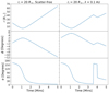 |
Fig. 1. Radial position (r), heliographic longitude (ϕ) and pitch angle (α) of a 300 MeV proton for the first 5 min of propagation under two different scattering conditions. The left column is for a scatter-free simulation, and the right column is for a proton from a simulation with a scattering mean free path of λ = 0.1 AU. Both simulations had injection at ri = 20 R⊙. Two scattering events occur in the right hand side panels at ∼3.5 and ∼4 min. |
To study the effect of scattering on the mirror point radius, we simulated the propagation of a population of 300 MeV protons with mean free path λ = 0.1 AU. For each proton injected into the simulation the mirror point was determined by identifying the minimum radial distance the particle reached. Figure 2 shows the mirror point radius, rmp versus initial pitch angle αi for the cases ri = 10, 20 and 30 R⊙. For clarity, only a subset of data points were plotted for each simulation. The purple, orange and green dashed lines give the scatter-free analytical value of rmp, according to Eq. (2). A number of data points were found to lie along these lines, corresponding to protons that did not scatter in the simulation, validating our code and methodology for deriving rmp. The blue dashed line at 1 R⊙ displays the height in the solar atmosphere that the protons must reach to go on to generate γ rays. Data points not along the curved dashed lines correspond to protons that experienced scattering.
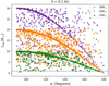 |
Fig. 2. Mirror point radius, rmp, versus particle initial pitch angle, αi for simulations with injections at 10 R⊙ (green circles), 20 R⊙ (orange squares) and 30 R⊙ (purple triangles) with λ = 0.1 AU. The green, orange, and purple dashed lines show the analytical, scatter-free mirror point radius, given by Eq. (2). The horizontal blue dashed line denotes the required depth in the solar atmosphere the protons must reach to generate γ rays (1 R⊙). |
In Fig. 2 there were a number of data points at or below the 1 R⊙ blue dashed line; these protons would be candidates to go on to produce γ rays. It is clear from Fig. 2 that they are a small fraction of the population. In the scatter-free case only particles in the loss cone (αi close to 180°) reach the solar surface, while for the scattering case particles across the pitch angle distribution can reach it if scattered favourably.
Figure 2 shows that scattering allows the possibility for protons to propagate deeper into the solar atmosphere than they would have in scatter-free conditions (indicated by the points below the corresponding dashed line). These protons’ velocity vectors have been scattered such that their pitch angles have shifted towards 180° (i.e. more field aligned). However, there were also a number of points above the scatter-free prediction, where pitch angles were shifted close to 90° (or the particle was reflected by the scattering event), resulting in the proton mirroring further from the solar surface than it would have under scatter-free conditions. The question of whether scattering primarily helps or hinders protons in their back-precipitation to the photosphere is addressed in Sect. 3.2.
3. Precipitation from instantaneous injection at a given injection height
For a simulation in which N particles were injected at height ri, we define the instantaneous precipitation fraction P as the percentage of the injected population that reached rp, P = Np/N × 100, where Np is the number of protons that successfully precipitate. Unless otherwise specified, we study precipitation to rp = 1 R⊙. In our simulations we assume the velocity distribution to be isotropic at the location of injection. Table 1 gives values of Np and P for our simulations.
Instantaneous precipitation fractions for our simulations.
3.1. Scatter-free precipitation fraction
We first considered precipitation in the scatter-free case. In general, for an isotropic particle population propagating in a magnetic field increasing monotonically between ri and rp, the precipitation fraction is given by
![Mathematical equation: $$ \begin{aligned} {P_{\rm sf} = \frac{1}{2} \left[1 - \sqrt{1 - \frac{B_{i}}{B_{\rm p}}}\right] \times 100 \;\; (\%)}, \end{aligned} $$](/articles/aa/full_html/2022/02/aa42002-21/aa42002-21-eq5.gif) (3)
(3)
where Bi is the magnetic field strength at the position of injection and Bp is the magnetic field strength at the precipitation radius.
Close to the Sun the Parker spiral magnetic field can be approximated as a purely radial field (as given by Eq. (1) with Ω = 0). In this case for an isotropic proton population Eq. (3) becomes
![Mathematical equation: $$ \begin{aligned} P_{\rm sf} = \frac{1}{2} \left[1 - \sqrt{1 - \left(\frac{r_{\rm p}}{r_{\rm i}}\right)^2}\right] \times 100 \;\; (\%), \end{aligned} $$](/articles/aa/full_html/2022/02/aa42002-21/aa42002-21-eq6.gif) (4)
(4)
where ri is the radius of injection. Considering ri = 20 R⊙ and rp = 1 R⊙ Eq. (4) yields Psf = 0.063%.
For a Parker spiral magnetic field (Eq. (1)), not necessarily close to the Sun, Eq. (3) gives
![Mathematical equation: $$ \begin{aligned} P_{\rm psf} = \frac{1}{2}\left(1 - \left[1 -\sqrt{\frac{r_{\rm i}^{-4} + (a r_{\rm i})^{-2}}{r_{\rm p}^{-4} + (a r_{\rm p})^{-2}}}\right]^\frac{1}{2}\right) \times 100 \;\; (\%). \end{aligned} $$](/articles/aa/full_html/2022/02/aa42002-21/aa42002-21-eq7.gif) (5)
(5)
Considering ri = 20 R⊙ and rp = 1 R⊙ Eq. (5) also yields Ppsf = 0.063%. We carried out scatter-free simulations with ri = 20 R⊙ using our model and obtained an instantaneous precipitation fraction P = 0.062% (Table 1) in good agreement with the analytical value.
3.2. Precipitation fraction in the presence of scattering
We carried out simulations with N = 10 million protons propagating over 24 h in a variety of scattering conditions and derived instantaneous precipitation fractions to rp = 1.0 R⊙. Figure 3 shows P versus the scattering mean free path, λ, for injection at ri = 20 R⊙ (left panel) and ri = 70 R⊙ (right panel).
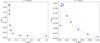 |
Fig. 3. Instantaneous precipitation fraction (P) versus scattering mean free path (λ). Left panel: instantaneous precipitation fraction (P) versus scattering mean free path λ from simulations with durations of 24 h, where protons were injected at a height of ri = 20 R⊙, and λ ranges from λ = 0.0025 AU to λ = 1.0 AU. The solar wind speed is vsw = 500 km s−1. Right panel: P versus λ for injections at 70 R⊙. Scattering mean free paths range from λ = 0.0025 AU to λ = 0.1 AU. Both panels were fitted with curves of the form of Eq. (6) with the left panel having constants; a = 0.0318 AU, b = 0.8287 and c = 0.0027 AU, and the right panel having constants; a = 0.0094 AU, b = 0.8054 and c = 0.0058 AU. |
The results show that increasing the amount of scattering does help precipitation, however, in the ri = 70 R⊙ case it is also evident that the efficiency of precipitation decreases at very small values of λ after a peak value is reached. By running a simulation at very small mean free path for ri = 20 R⊙ we verified that a peak in the P profile at low λ is present also in this case.
We find that a function of the form
 (6)
(6)
where a, b and c are positive constants, provides a good fit to the simulation points (blue dashed lines).
The peak in precipitation fraction results from the fact that when the scattering becomes very strong, outward convection with the solar wind overcomes the positive effects of enhanced scattering. As confirmation of this interpretation, a function similar to Eq. (6) can be obtained from solution of a transport equation including focussing, diffusion and convection, in the strong scattering limit (Earl 1974). From a test-particle model point of view, the peak corresponds to conditions that maximise the chances of particles scattering into the loss cone and remaining in it long enough to reach the precipitation radius. Any more scattering taking place ejects the particles from the loss cone too fast.
The position of the peak depends on injection height and solar wind speed. At larger ri the peak is reached at a larger λ because scattering effects have more time to play a part. We found from our simulations that P depends weakly on the solar wind speed, increasing with decreasing vsw, when all other parameters were kept constant. The value of λ at which P reaches a peak decreases for decreasing vsw.
For ri = 70 R⊙ (right panel) P reaches a peak value of P ∼ 0.22% at λ ∼ 0.0072 AU. In the case ri = 20 R⊙ (left panel), the fit indicates that the peak in precipitation fraction would be P ∼ 1.69% at λ = 0.0032 AU.
For medium/high values of λ (low scattering) there is a tendency for protons to precipitate soon after injection, which is quantified in the final column of Table 1. For the high λ case this is especially important as the protons that precipitate early represent a very large percentage of the total number of successfully precipitating protons. We define F10 min as the percentage of the total precipitating protons over the full simulation (24 h), Np, that precipitate in the first 10 min. The last column in Table 1 gives F10 min for our simulations. For a simulation with ri = 20 R⊙ and λ = 0.1 AU F10 min ∼ 69%. For the same injection location, when λ = 0.01 AU, this drops dramatically to F10 min ∼ 25%. However, a greater number of protons than the λ = 0.1 AU simulation reach the solar surface over the first 10 min for λ = 0.01 AU because precipitation is more efficient. As expected, more turbulent magnetic fields lead to smaller F10 min values as protons are slowed due to more frequent scattering events. Simulations with injections close to the solar surface have high F10 min values, for instance F10 min ∼ 96% for a simulation with, ri = 5 R⊙, λ = 0.1 AU. This percentage decreases with increasing radial position of the injection region (see Table 1).
In addition to modelling back-precipitation to rp = 1 R⊙ we also ran simulations with protons propagating to rp = 2.5 R⊙, corresponding to the height of the source surface, from where a model of coronal and photospheric magnetic fields would need to be used to obtain a more precise estimate of precipitation fractions to the photosphere. Precipitation fractions to the source surface were found to be about 5 times larger compared to those shown in Fig. 3.
3.3. Dependence of P on injection height
Having studied the dependence of P on the scattering conditions, we focussed on a specific mean free path value, λ = 0.1 AU and investigate the radial dependence of P with injection height. Fig. 4 shows P versus ri, characterised by a sharp decline with increasing injection height, due to the stronger magnetic mirror effect. Scattering results were compared with the scatter-free curve (blue line). The simulation points can be fit by
![Mathematical equation: $$ \begin{aligned} P(r_{\rm i}) = 31.084\left(1-\left[1-\sqrt{\frac{(r_{\rm i}^{-2.990} + a^{-2} r_{\rm i}^{0.035})}{(r_{\rm p}^{-4} + (a r_{\rm p})^{-2})}}\right]^{1/2}\right), \;\;(\%) \end{aligned} $$](/articles/aa/full_html/2022/02/aa42002-21/aa42002-21-eq9.gif) (7)
(7)
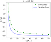 |
Fig. 4. Instantaneous precipitation fraction (P) versus radial location of injection (ri) for scattering described by a mean free path λ = 0.1 AU. The points have been fitted with the line described by Eq. (7), and the blue curve represents scatter-free precipitation according to Eq. (5). |
where ri is in solar radii. As the shock-source propagates from 5 to 70 R⊙ the precipitation fraction from our simulations drops from 1.450% to 0.058%. This corresponds to a drop in the number of protons reaching the solar surface by a factor of ∼25 assuming an injection function that is constant with ri.
Equation (7) is a proxy for the temporal evolution of the instantaneous precipitation fraction. Depending on its speed, each CME-driven shock will cover the range of radial distances in Fig. 4 over timescales that are unique to that event. Hence, the shock-height versus time curve determines the temporal evolution of the instantaneous precipitation fraction.
4. Evaluation of emission region features
In Fig. 5 the locations where the protons crossed the 1 R⊙ boundary are displayed for two particle energies (300 MeV (top panels) and 1 GeV (bottom panels)) and scattering mean free paths of λ = 0.1 AU (panels a and c) and λ = 0.01 AU (panels b and d) in a coordinate system corotating with the Sun. The red square is the region of the photosphere directly connected to the injection region. All simulations had injections located at ri = 20 R⊙.
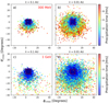 |
Fig. 5. Heliographic latitude ( |

In Fig. 5 panels a and c there is a systematic drift of the crossing position southwards with time. The same trend is seen in Fig. 5 panels b and d. However, some crossings were also observed northwards of the emission region. The southward drift is due to gradient and curvature drifts associated with the Parker spiral magnetic field (Dalla et al. 2013). For our magnetic polarity this leads to a southward drift; however, in the opposite magnetic polarity these drifts would be northwards. In addition, finite Larmor radius effects associated with scattering events produce motion of the guiding centre perpendicular to the magnetic field. The finite Larmor radius effects were more prominent in the λ = 0.01 AU panels and they were the cause of the northward displacement. We note that the finite Larmor radius effects do not have a preferential direction unlike the drifts. They were expected to be more prominent in the more magnetically turbulent simulations as the proton can shift up to 2 Larmor radii per scattering event and there were more scattering events in these simulations.
The longitudinal and latitudinal positions of the protons reiterate that they do not propagate solely along the Parker spiral lines they were initially accelerated on. Therefore, drifts and finite Larmor radius effects are not negligible when determining if protons from the shock are responsible for the observed position of the γ ray emission region on the solar disc, especially in the high scattering case. Higher-energy protons show stronger deviations from their original Parker spiral field lines, even for earlier precipitating protons, due to the increase in drifts and finite Larmor radius effects with increasing particle energy. This is clear when comparing panels c and d with panels a and b in Fig. 5.
When considering injections at larger radial distances we found that, as expected, the emission region moves westwards. This occurs as the CME-driven shock propagates to larger radial distances it injects particles onto Parker spiral lines with footpoints located increasingly westwards on the photosphere.
We note that we have only considered a unipolar Parker spiral magnetic field. Positions on the solar disc are likely to be altered by the more complex coronal magnetic field structure.
5. Shock heights during LDGRF events
We now apply the results of our simulations to a set of eight specific LDGRF events: the subset of events from the Winter et al. (2018) study with a > 2 h duration. These events are listed and discussed further in Sect. 6 (see Table 2). They were associated with CMEs with plane-of-the-sky speeds ranging from 950 to 2684 km s−1 based on the Coordinated Data Analysis Workshops (CDAW1) catalogue of observations by the Large Angle and Spectrometric Coronagraph (LASCO) on board the Solar and Heliospheric Observatory (SOHO).
For each of the eight LDGRF events we estimate the position of the shock at the time of peak and end γ ray emission, using CME data and a series of approximations. We assumed that the shock height and speed coincide with those of the associated CME and that all parts of the shock propagate radially. We used the linear fit in the CDAW catalogue to determine height versus time for r < 30 R⊙. At larger distances we used the empirical expression of Gopalswamy et al. (2001) to describe the shock’s acceleration (or deceleration), ash, during the propagation to 1 AU:
 (8)
(8)
where ash is in m s−2 and vsh is the shock speed in km s−1. According to this equation shocks faster than ∼406 km s−1 decelerate. All the shocks listed in Table 2 were significantly faster than this and so decelerate during their propagation. To obtain the peak times of the γ ray emission we used data from Table 3 of Share et al. (2018) and the corresponding plots in their Appendix C, and for the end times we used data from Table 1 of Winter et al. (2018).
For the eight LDGRF events the shock positions at the peak and end times of the γ ray emission were plotted in Fig. 6 as circles and squares respectively. Here the shaded wedges span 500 km s−1 increments in constant shock speed from 500 to 3000 km s−1. For the 2012 March 7 event, which was associated with two fast CMEs erupting in rapid succession, data points for both (with speeds of 2684 km s−1 and 1825 km s−1, respectively) were plotted. While the absence of interplanetary type III radio emissions during the second, much slower CME suggests that it was unlikely associated with the SEP event at 1 AU (see Richardson et al. 2014), a direct contribution to particle acceleration cannot be ruled out, so both CMEs were considered.
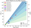 |
Fig. 6. Radial distance, r, from the centre of the Sun of CME-driven shocks associated with LDGRFs at the peak times (circles) and end times (squares) of detected γ ray emission. Constant deceleration is assumed during propagation, as given by Eq. (8), and initial plane-of-the-sky speeds were taken from the SOHO/LASCO CME catalogue. Each shaded wedge spans 500 km s−1 increments in radial shock speed between 500 and 3000 km s−1. For the 2012 March 7 event we show two sets of radial positions for two different CME-driven shocks that day: 2012-Mar-07(a) is the earlier, faster CME with a speed of 2684 km s−1 and 2012-Mar-07(b) is the second, slower CME with a speed 1825 km s−1. |
Figure 6 shows that if the CME-driven shock was the source of the γ ray emission in the LDGRF events, back-precipitation from large distances needs to have taken place. The median position of the shock at the end time is ∼71 R⊙ (including both shocks that originated on 2012 March 7). For the 2012 March 7 event the two associated shocks were located at ∼242 R⊙ and ∼155 R⊙ at the end time of the γ ray emission, which lasted for 19.5 h.
6. Total precipitation fraction
In this section we combine our simulation results for the instantaneous precipitation fraction as a function of ri (as summarised in Fig. 4) with the information on shock height versus time for LDGRF events to obtain an upper limit estimate,  , of the total precipitation fraction in the events, within the CME shock scenario. We calculate
  as
as
 (9)
(9)
where P(ri) describes the radial evolution of the instantaneous precipitation fraction (Eq. (7)), N(ri) the number of injected particles as a function of radial distance (injection function), rini the radial position of the shock when particle acceleration begins, and rfin the position when particle acceleration ends. Hence,  is the ratio of the total number of precipitating and injected protons over the event.
For P(ri) we make use of the fit of the curve in Fig. 4 (Eq. (7)), corresponding to scattering conditions described by λ = 0.1 AU, (i.e. strong scattering). We used a simple model for the injection function given by
 (10)
(10)
where A, B and C are positive constants. This functional form describes a fast rise phase to peak injection, then a turnover and subsequent slow decay, describing the fact that energetic particles are more efficiently accelerated when the shock is closer the Sun. In particular, in the scatter free hypothesis and the CME shock acceleration scenario the highest-energy particles associated with Ground Level Enhancements are thought to typically be released at shock heights of 2−4 R⊙ (Reames 2009; Gopalswamy et al. 2013a).
To calculate  we need to specify rini and rfin in Eq. (9). Conservatively, we assume that particle acceleration begins at the radial position of the formation of the shock. Gopalswamy et al. (2013b) determined the median shock formation height of 1.20 R⊙, which we considered as a possible estimate for rini. We estimate rfin by calculating the shock position at the time when the γ ray emission ends (based on the observed durations). The values of rfin for the LDGRF events are shown in Col. 4 in Table 2 and plotted in Fig. 6.
6.1. Influence of injection function on precipitation
Figure 7 shows the effect of injection function shape on  . Here N(ri) for different values of A, B and C and a fixed radial position of peak injection, rpeak = 5.0 R⊙ are shown. The injection functions are normalised so that the total number of injected particles was the same for different curves. The right panel of Fig. 7 displays the corresponding total precipitation fractions, determined using Eq. (9), where each coloured point represents the
  of the same coloured curve in the left panel. Here we used rini = 1.20 R⊙ and rfin = 70.91 R⊙, the latter being the median end time position of the shocks of Table 2.
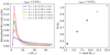 |
Fig. 7. Normalised injection functions (left panel) with peak injection at 5.0 R⊙ and differing decay rates versus the radial position of the shock, ri. Only values of N(ri) > 0.001 were plotted for clarity. The corresponding total precipitation fraction ( |


We note that for a delta function injection the total precipitation fraction is the same as the instantaneous precipitation fraction given by Eq. (7). It is clear from Fig. 4 that the further from the Sun particles are injected the harder it is for them to back-precipitate. Therefore, the more sunwards the injection function is skewed the larger the total precipitation fraction is (i.e. peak injection occurring closer to the Sun leads to higher  and extended injections reduce
  ). This is identifiable by comparing the blue and purple injection functions and their corresponding
  in Fig. 7. The blue and purple injection functions in the left panel have total precipitation fractions of 0.459% and 1.025%, respectively. The extended decay phase of the blue curve skews the injection further from the Sun where the efficiency of the back-precipitation is low, resulting in the lower total precipitation fraction.
Figure 7 shows that for large total precipitation fractions a prompt injection close to the solar surface is required. However, this will result in shorter durations of γ ray emission. Conversely, injections extended over large radial distances will provide longer durations of γ ray emission at the expense of the total precipitation fraction. Therefore, large precipitation fractions and long durations of γ ray emission cannot be reconciled using the CME-driven shock acceleration scenario.
6.2. Total precipitation fraction for eight LDGRF events
We calculated  from Eq. (9) using an injection described by Eq. (10) with A = 1.0 R⊙, B = 1.58 and C = 6.0 R⊙, corresponding to the red curve in Fig. 7. The injection was normalised such that the same number of particles were considered for each injection. The values for
  we obtained are displayed in the final column of Table 2, corresponding to rini = 1.20 R⊙, for the eight LDGRF events. These values are small, ranging from
  to ∼0.93%, with the smallest
  values associated with the events with the fastest shocks or longest durations. As indicated by Fig. 7 if the injection was more prompt (like the purple curve in Fig. 7) then larger
  values are possible. Similarly, if the injection was more sunwards-skewed the
  values would increase further. We considered the effect of an injection with rpeak = 3.0 R⊙, keeping all parameters the same, and
  increased to ∼2%.
The total precipitation fraction of the event,  , becomes smaller if acceleration at the CME shock continues over larger distances, as can be seen from Table 2 considering the events with the largest values of rfin. Typically these are the events with very long durations, very fast shocks or both. Looking at the two shocks associated with the 2012 March 7 event one can see that having a slower shock over the same duration will lead to an increased
  . We note that if the proton acceleration occurs at the flanks of the shock this would increase the
  as they remain closer to the solar surface than the shock nose. However, higher-energy particles are believed to be more efficiently accelerated over a small shock region around the nose (Zank et al. 2006; Hu et al. 2017).
7. Time profiles of proton back-precipitation
The test particle simulations described in Sect. 3 have considered injection at a single radial position, rather than a moving shock. To derive information about how precipitation evolves over time, we also carried out a test-particle simulation with moving shock-like injection (Hutchinson et al. 2021). We considered a shock with radial speed of 2684 km s−1 at 1.2 R⊙ that injects particles over the radial distance range 1.2−228.6 R⊙ and follows the injection function given in Eq. (10) with A = 1.0 R⊙, B = 1.58 and C = 6.0 R⊙. This injection approximates the injection for the fastest shock in the 2012 March 7 event, with the acceleration of energetic protons occurring over 19.5 h. We assume constant shock deceleration as described in Sect. 5.
The time profile of precipitation can be seen in Fig. 8. Data points from Fermi/LAT showing the time evolution of the γ ray emission are also shown. It can be seen that even for an extended injection, in the simulations the majority of back-precipitation takes place early. The rapid decay in precipitation highlights the significant challenge that magnetic mirroring poses to back-precipitating protons.
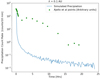 |
Fig. 8. Precipitation count rate versus time from a simulation with injection from a moving shock-like source with the same speed as the fastest 2012 March 7 shock (blue line), at 10 min resolution. The radial profile of particle injection is given by Eq. (10) with A = 1.0 R⊙, B = 1.58 and C = 6.0 R⊙. Green data points show the time evolution of the γ ray emission, from Ajello et al. (2014). |
As can be seen from Fig. 8, the precipitation drops by three orders of magnitude within ∼5 h, even though injection continues for many hours beyond this. According to the γ ray profile for the 2012-03-07 event (Ajello et al. 2014), the detected γ ray emission drops by only ∼2 orders of magnitude over the 19.5 h duration of the LDGRF event. This injection considers the fastest shock associated with the 2012-03-07 LDGRF event. We also considered the contribution from the slower second shock (not displayed in Fig. 8), where we find that it decays much faster than the decay of the observed γ ray profile.
8. Discussion and conclusions
Energetic (> 300 MeV) proton back-propagation from CME heights down to the solar surface is strongly impeded by magnetic mirroring. In this paper we investigated whether scattering associated with turbulence may aid back-precipitation to the levels required to explain LDGRFs via the CME shock scenario, by ensuring that more particles enter the loss cone. We investigated the problem extensively using 3D test particle simulations with varying levels of scattering.
Particles accelerated at a CME-driven shock may back-precipitate via a number of different routes. There might be the possibility of almost scatter-free trajectories or propagation might be strongly influenced by the scattering behind the shock. In some cases back-precipitation from the flanks may be involved. We found that compared to the scatter-free case, scattering does enhance particle precipitation. For example for injection at ri = 20 R⊙ it increases the instantaneous precipitation fraction P from 0.06% (scatter-free) to 0.21% for a mean free path λ = 0.1 AU. Increasing the level of scattering further improves the precipitation fraction to, for example ∼P = 1.63% when λ = 0.0025 AU. There is, however, a limit to this increase because when the scattering mean free path becomes very small outward convection with the solar wind becomes very efficient and particles can no longer back-precipitate (as shown in Fig. 3). The value of the mean free path at which this effect becomes significant is dependent on injection height and solar wind speed. In our simulations the convection effect becomes important for mean free paths below 0.0072 AU for ri = 70 R⊙ and below 0.0032 AU for ri = 20 R⊙.
Some studies in the literature have assumed very strong scattering conditions behind the shock, for shock heights up to ∼10 R⊙. For example, Afanasiev et al. (2018) used a model where λ increases from 0 at the shock front up to a maximum value λ0 at the Sun, where λ0 varies in the range 0.16 ≤ λ0 ≤ 3.2 R⊙ (∼0.0007 ≤ λ0 ≤ ∼0.015 AU) across different simulations. Jin et al. (2018) suggest that a mean free path of the order of 1 R⊙ (∼0.0047 AU) is sufficient to overcome the strong magnetic mirroring that occurs close to the Sun. While this may be the case very close to the Sun, our results show that when the shock is further out very small mean free paths impede back-propagation via the outward convection effect. When shock locations further from the Sun are considered very low mean free path values are probably unrealistic. If the scattering were very strong all the way from the shock to the corona, many hours after CME liftoff, one would expect to observe a long lasting increase in SEP fluxes after the passage of the CME driven shock at a near-Sun spacecraft. To our knowledge this has never been seen, for instance in data from the Helios 1 and 2 spacecraft (e.g. Kallenrode 1993). It is hoped that new data from Parker Solar Probe and Solar Orbiter will provide additional information on this question. When studying total precipitation fractions (Sect. 6) we assumed λ = 0.1 AU, similar to typical mean free paths that have been derived by fits of ground level enhancement measurements, due to > 500 MeV protons (e.g. λ = 0.27 AU used by Bieber et al. 2002).
Overall, even in the presence of scattering, back-precipitation is generally highly inefficient, with instantaneous precipitation fractions being below 2% in our simulations. P decreases strongly with height of injection, ri (Fig. 4) because of this proton injection at large radial distances cannot meaningfully extend the precipitation on the solar surface.
It is also possible to use the results of our simulations, specifically the radial dependence of instantaneous precipitation, to estimate an upper limit  to the total precipitation fraction within the CME shock scenario. Using a variety of idealised injection functions we have shown that when the acceleration takes place over a broad range of radial distances, for example in the case of very fast shocks, lower values of
  are obtained. When
  was calculated for eight solar eruptive events that resulted in LDGRFs the values obtained range from ∼0.56% to ∼0.93%, with the smallest values corresponding to events with the fastest shocks and longer durations. This is because the shocks for these events spend less time close to the solar surface, where the precipitation is efficient. The radial position of initial particle injection (rini) has a substantial effect on the total precipitation fraction. All the events analysed were associated with fast CME-driven shocks: a shock with the average speed of our subset of events could reach 70 R⊙ in less than 6.7 h. The fastest shock would cover this distance in ∼5 h.
de Nolfo et al. (2019) used observations to directly compare the number of protons interacting at the Sun, NLDGRF, with the number of SEP protons at 1 AU, NSEP. From NLDGRF and NSEP they calculated a lower limit on the total precipitation fraction required for the validity of the CME shock scenario, in which the two populations have a common origin. They found that precipitation fractions greater than 10% were required in the majority of the 14 events considered, as shown by their Fig. 8. For the 2011 March 7 and 2012 January 23 events they reported that a > 90% precipitation fraction is required by the CME scenario. Our modelling of the same events found values more than two orders of magnitude smaller, with  ∼ 0.60% and ∼0.67%, respectively. The small value (∼2.9%) they obtained for the 2014 February 25 event is approximately a factor of 4.5 greater than our estimate (∼0.64%). In the case of the 2012 March 7–10 events, since it was not possible to evaluate the individual contributions in terms of SEP intensities at 1 AU, they provided a single precipitation fraction value of ∼18%, which exceeds by at least 19 times the values that we calculated for three CMEs on 2012 March 7–9 considered in this work (∼0.56 − 0.93%); similar results are expected for the 2012 March 10 CME, characterised by an intermediate speed. Overall we conclude that while in many events the direct observational comparison between the interacting and SEP populations gives rise to a requirement of large precipitation fractions under the assumption of CME shock acceleration of both populations (de Nolfo et al. 2019), for the same events our modelling cannot produce them due to the strong effect of magnetic mirroring. This poses a problem for the CME shock hypothesis for LDGRFs.
In order to obtain larger precipitation fractions from our model for the eight LDGRF events we would have to choose the injection function with fastest rise and shortest decay phase (i.e. tending towards a delta function injection at the radial position of peak injection – an instantaneous injection), but the result of this would be a reduction in the overall duration of precipitation. Even with this choice of injection function  would overall still remain smaller than 1.5% (for our peak injection at 5.0 R⊙, see Table 1).
Our simulations also show that with increasing radial distance of injection the emission region on the solar surface moves westwards. Particles that precipitate early in time after injection tend to follow Parker spiral magnetic field lines, but with increasing propagation time the protons deviate due to drifts and finite Larmor radius effects. This deviation becomes larger with increasing particle energy (Fig. 5).
Our estimates of the proton precipitation count rate due to the first shock in the 2012 March 7 event (Fig. 8) decay much faster than even the comparatively rapid early decay of the observed γ ray profile, and contributions towards the precipitation quickly fall orders of magnitude indicating that γ ray production due to the back-precipitation of energetic protons from a CME driven-shock is inconsistent with the long duration of the observed γ ray profiles for λ = 0.1 AU.
In summary the above results present a challenge to the CME shock acceleration scenario for LDGRFs as follows:
-
Long after the eruptive event, CME shocks are very far from the solar surface and back-precipitation is extremely difficult. A faster CME shock only exacerbates this problem.
-
The total precipitation fraction,
 , values obtained in our study were typically smaller than 1.5%, while work by de Nolfo et al. (2019) has indicated that in several LDGRF events a much larger value of
  is required for the validity of the CME shock scenario.
 -
Time-extended acceleration and large total precipitation fractions cannot be reconciled according to our simulations. A model of an event that makes the duration of the acceleration longer will result in smaller total precipitation fractions.
-
The specific shape of the precipitation count rate versus time obtained from our simulations displays a much faster decay than that observed in LDGRF intensity profiles (Fig. 8).
In our simulations 300 MeV protons were considered. However, we do not expect a significant difference in total precipitation fractions for higher-energy particles as scattering depends on energy only weakly and the magnetic mirror effect does not depend on particle energy.
The shock speeds used to calculate the  values were based on the plane-of-the-sky CME speeds averaged over the LASCO field of view (2−32 R⊙). Therefore, they underestimate the CME velocities close to the Sun and, in general, the corresponding space (3D) speeds due to projection effects, especially for events originating far from the solar limb. Consequently, derived total precipitation fractions are expected to be overestimates. However, their values remain very small even with these assumptions.
In this paper we did not consider the expansion of the magnetic field in the corona and near the photosphere and their effects on particle back-precipitation. The coronal magnetic field is complex and modelling it accurately involves using either an MHD simulation or a potential field source surface model. These types of simulations show significant expansion of the magnetic field, which provides an increased challenge to charged particles that attempt to propagate deep into the solar atmosphere. Below the corona the magnetic field penetrates the photosphere at the edges of the convective cells and forms a ‘canopy’ at the base of the corona, where magnetic pressure dominates (Seckel et al. 1991, 1992). The result of the magnetic field being swept to the edges of convective cells is an inhomogeneous magnetic field, with flux ‘bundles’ having magnetic field strengths of the order of 103 Gauss, while the average magnetic field strength of the photosphere is of the order of a few Gauss (Seckel et al. 1991). Therefore, particles propagating through coronal and photospheric magnetic fields will experience increased mirroring, not considered in this study. Including these effects will reduce the precipitation fractions further due to the large mirror ratio associated with the inhomogeneous magnetic field structure. We plan to address this question in future work.
Further work is required to fully understand the contribution of the CME shock scenario to the production of γ rays during LDGRFs. Modelling events in detail, especially the complex events that are more difficult to explain using the shock source scenario, such as the 2012 March 7 event, would provide a clearer picture of its contribution. In further work we will examine the effects of including the Heliospheric current sheet and current sheets in the vicinity of the CME in future modelling.
Acknowledgments
A. Hutchinson, S. Dalla and T. Laitinen acknowledge support from the UK Science and Technology Facilities Council (STFC), through a Doctoral Training grant – ST/T506011/1 and grants ST/R000425/1 and ST/V000934/1. C. O. G. Waterfall and S. Dalla acknowledge support from NERC grant NE/V002864/1. G. A. de Nolfo and A. Bruno are supported by the NASA Goddard Space Flight Center/Internal Scientist Funding Model (ISFM) grant HISFM18. This work was performed using resources provided by the Cambridge Service for Data Driven Discovery (CSD3) operated by the University of Cambridge Research Computing Service (www.csd3.cam.ac.uk), provided by Dell EMC and Intel using Tier-2 funding from the Engineering and Physical Sciences Research Council (capital grant EP/P020259/1), and DiRAC funding from the Science and Technology Facilities Council (www.dirac.ac.uk).
References
- Ackermann, M., Allafort, A., Baldini, L., et al. 2017, ApJ, 835, 219 [CrossRef] [Google Scholar]
- Afanasiev, A., Aran, A., Vainio, R., et al. 2018, in Solar Particle Radiation Storms Forecasting and Analysis, eds. O. E. Malandraki, & N. B. Crosby, 444, 157 [NASA ADS] [CrossRef] [Google Scholar]
- Ajello, M., Albert, A., Allafort, A., et al. 2014, ApJ, 789, 20 [NASA ADS] [CrossRef] [Google Scholar]
- Bieber, J. W., Droge, W., Evenson, P. A., et al. 2002, ApJ, 567, 622 [NASA ADS] [CrossRef] [Google Scholar]
- Cane, H. V. 1988, J. Geophys. Res.: Space Phys., 93, 1 [NASA ADS] [CrossRef] [Google Scholar]
- Cliver, E. W., Kahler, S. W., & Vestrand, W. T. 1993, Int. Cosm. Ray Conf., 3, 91 [NASA ADS] [Google Scholar]
- Dalla, S., Marsh, M., Kelly, J., & Laitinen, T. 2013, J. Geophys. Res.: Space Phys., 118, 5979 [NASA ADS] [CrossRef] [Google Scholar]
- Dalla, S., de Nolfo, G. A., Bruno, A., et al. 2020, A&A, 639, A105 [NASA ADS] [CrossRef] [EDP Sciences] [Google Scholar]
- de Nolfo, G. A., Bruno, A., Ryan, J. M., et al. 2019, ApJ, 879, 90 [NASA ADS] [CrossRef] [Google Scholar]
- Earl, J. A. 1974, ApJ, 193, 231 [NASA ADS] [CrossRef] [Google Scholar]
- Gopalswamy, N., Lara, A., Yashiro, S., Kaiser, M. L., & Howard, R. A. 2001, J. Geophys. Res.: Space Phys., 106, 29207 [Google Scholar]
- Gopalswamy, N., Xie, H., Akiyama, S., et al. 2013a, ApJ, 765, L30 [NASA ADS] [CrossRef] [Google Scholar]
- Gopalswamy, N., Xie, H., Mäkelä, P., et al. 2013b, Adv. Space Res., 51, 1981 [NASA ADS] [CrossRef] [Google Scholar]
- Grechnev, V. V., Kiselev, V. I., Kashapova, L. K., et al. 2018, Sol. Phys., 293, 133 [NASA ADS] [CrossRef] [Google Scholar]
- Hu, J., Li, G., Ao, X., Zank, G. P., & Verkhoglyadova, O. 2017, J. Geophys. Res.: Space Phys., 122, 10,938 [Google Scholar]
- Hudson, H. S. 2018, in Space Weather of the Heliosphere: Processes and Forecasts, eds. C. Foullon, & O. E. Malandraki, IAU Symp., 335, 49 [NASA ADS] [Google Scholar]
- Hutchinson, A., Dalla, S., Laitinen, T., & Waterfall, C. 2021, in Proceedings of 37th International Cosmic Ray Conference – PoS(ICRC2021), ed. B. Keilhauer, Proc. Sci., 395, 1313 [CrossRef] [Google Scholar]
- Jin, M., Petrosian, V., Liu, W., et al. 2018, ApJ, 867, 122 [CrossRef] [Google Scholar]
- Kahler, S. W. 2016, ApJ, 819, 105 [NASA ADS] [CrossRef] [Google Scholar]
- Kahler, S. W., Cliver, E. W., & Kazachenko, M. 2018, ApJ, 868, 81 [CrossRef] [Google Scholar]
- Kallenrode, M.-B. 1993, J. Geophys. Res., 98, 19037 [NASA ADS] [CrossRef] [Google Scholar]
- Klein, K.-L., Tziotziou, K., Zucca, P., et al. 2018, in Solar Particle Radiation Storms Forecasting and Analysis, eds. O. E. Malandraki, & N. B. Crosby, 444, 133 [NASA ADS] [CrossRef] [Google Scholar]
- Kocharov, L., Laitinen, T., Vainio, R., et al. 2015, ApJ, 806, 80 [NASA ADS] [CrossRef] [Google Scholar]
- Kong, X., Guo, F., Chen, Y., & Giacalone, J. 2019, ApJ, 883, 49 [NASA ADS] [CrossRef] [Google Scholar]
- Kouloumvakos, A., Rouillard, A. P., Share, G. H., et al. 2020, ApJ, 893, 76 [CrossRef] [Google Scholar]
- Mandzhavidze, N., & Ramaty, R. 1992, ApJ, 396, L111 [CrossRef] [Google Scholar]
- Marsh, M. S., Dalla, S., Kelly, J., & Laitinen, T. 2013, ApJ, 774, 4 [NASA ADS] [CrossRef] [Google Scholar]
- Masson, S., Démoulin, P., Dasso, S., & Klein, K. L. 2012, A&A, 538, A32 [NASA ADS] [CrossRef] [EDP Sciences] [Google Scholar]
- Omodei, N., Pesce-Rollins, M., Longo, F., Allafort, A., & Krucker, S. 2018, ApJ, 865, L7 [NASA ADS] [CrossRef] [Google Scholar]
- Owens, M. J., & Forsyth, R. J. 2013, Liv. Rev. Sol. Phys., 10, 5 [Google Scholar]
- Pesce-Rollins, M., Omodei, N., Petrosian, V., et al. 2015, ApJ, 805, L15 [NASA ADS] [CrossRef] [Google Scholar]
- Reames, D. V. 2009, ApJ, 706, 844 [NASA ADS] [CrossRef] [Google Scholar]
- Richardson, I. G., von Rosenvinge, T. T., Cane, H. V., et al. 2014, Sol. Phys., 289, 3059 [NASA ADS] [CrossRef] [Google Scholar]
- Ryan, J. M. 2000, Space Sci. Rev., 93, 581 [NASA ADS] [CrossRef] [Google Scholar]
- Ryan, J. M., & Lee, M. A. 1991, ApJ, 368, 316 [NASA ADS] [CrossRef] [Google Scholar]
- Seckel, D., Stanev, T., & Gaisser, T. K. 1991, ApJ, 382, 652 [CrossRef] [Google Scholar]
- Seckel, D., Stanev, T., & Gaisser, T. K. 1992, NASA Conf. Publ., 3137, 542 [NASA ADS] [Google Scholar]
- Share, G. H., Murphy, R. J., White, S. M., et al. 2018, ApJ, 869, 182 [NASA ADS] [CrossRef] [Google Scholar]
- Winter, L. M., Bernstein, V., Omodei, N., & Pesce-Rollins, M. 2018, ApJ, 864, 39 [NASA ADS] [CrossRef] [Google Scholar]
- Zank, G. P., Li, G., Florinski, V., et al. 2006, J. Geophys. Res.: Space Phys., 111 [CrossRef] [Google Scholar]
All Tables
All Figures
|
Fig. 1. Radial position (r), heliographic longitude (ϕ) and pitch angle (α) of a 300 MeV proton for the first 5 min of propagation under two different scattering conditions. The left column is for a scatter-free simulation, and the right column is for a proton from a simulation with a scattering mean free path of λ = 0.1 AU. Both simulations had injection at ri = 20 R⊙. Two scattering events occur in the right hand side panels at ∼3.5 and ∼4 min. |
| In the text | |
|
Fig. 2. Mirror point radius, rmp, versus particle initial pitch angle, αi for simulations with injections at 10 R⊙ (green circles), 20 R⊙ (orange squares) and 30 R⊙ (purple triangles) with λ = 0.1 AU. The green, orange, and purple dashed lines show the analytical, scatter-free mirror point radius, given by Eq. (2). The horizontal blue dashed line denotes the required depth in the solar atmosphere the protons must reach to generate γ rays (1 R⊙). |
| In the text | |
|
Fig. 3. Instantaneous precipitation fraction (P) versus scattering mean free path (λ). Left panel: instantaneous precipitation fraction (P) versus scattering mean free path λ from simulations with durations of 24 h, where protons were injected at a height of ri = 20 R⊙, and λ ranges from λ = 0.0025 AU to λ = 1.0 AU. The solar wind speed is vsw = 500 km s−1. Right panel: P versus λ for injections at 70 R⊙. Scattering mean free paths range from λ = 0.0025 AU to λ = 0.1 AU. Both panels were fitted with curves of the form of Eq. (6) with the left panel having constants; a = 0.0318 AU, b = 0.8287 and c = 0.0027 AU, and the right panel having constants; a = 0.0094 AU, b = 0.8054 and c = 0.0058 AU. |
| In the text | |
|
Fig. 4. Instantaneous precipitation fraction (P) versus radial location of injection (ri) for scattering described by a mean free path λ = 0.1 AU. The points have been fitted with the line described by Eq. (7), and the blue curve represents scatter-free precipitation according to Eq. (5). |
| In the text | |
|
Fig. 5. Heliographic latitude ( |
| In the text | |
|
Fig. 6. Radial distance, r, from the centre of the Sun of CME-driven shocks associated with LDGRFs at the peak times (circles) and end times (squares) of detected γ ray emission. Constant deceleration is assumed during propagation, as given by Eq. (8), and initial plane-of-the-sky speeds were taken from the SOHO/LASCO CME catalogue. Each shaded wedge spans 500 km s−1 increments in radial shock speed between 500 and 3000 km s−1. For the 2012 March 7 event we show two sets of radial positions for two different CME-driven shocks that day: 2012-Mar-07(a) is the earlier, faster CME with a speed of 2684 km s−1 and 2012-Mar-07(b) is the second, slower CME with a speed 1825 km s−1. |
| In the text | |
|
Fig. 7. Normalised injection functions (left panel) with peak injection at 5.0 R⊙ and differing decay rates versus the radial position of the shock, ri. Only values of N(ri) > 0.001 were plotted for clarity. The corresponding total precipitation fraction ( |
| In the text | |
|
Fig. 8. Precipitation count rate versus time from a simulation with injection from a moving shock-like source with the same speed as the fastest 2012 March 7 shock (blue line), at 10 min resolution. The radial profile of particle injection is given by Eq. (10) with A = 1.0 R⊙, B = 1.58 and C = 6.0 R⊙. Green data points show the time evolution of the γ ray emission, from Ajello et al. (2014). |
| In the text | |
Current usage metrics show cumulative count of Article Views (full-text article views including HTML views, PDF and ePub downloads, according to the available data) and Abstracts Views on Vision4Press platform.
Data correspond to usage on the plateform after 2015. The current usage metrics is available 48-96 hours after online publication and is updated daily on week days.
Initial download of the metrics may take a while.