| Issue |
A&A
Volume 657, January 2022
|
|
|---|---|---|
| Article Number | A130 | |
| Number of page(s) | 15 | |
| Section | Celestial mechanics and astrometry | |
| DOI | https://doi.org/10.1051/0004-6361/202142365 | |
| Published online | 21 January 2022 | |
An estimation of the Gaia EDR3 parallax bias from stellar clusters and Magellanic Clouds data
Centro de Astrobiología,
CSIC-INTA. Campus ESAC. C. bajo del castillo s/n. 28 692 Villanueva de la Cañada,
Madrid,
Spain
e-mail: jmaiz@cab.inta-csic.es
Received:
4
October
2021
Accepted:
4
November
2021
Context. The early-third Gaia data release (EDR3) parallaxes constitute the most detailed and accurate dataset that currently can be used to determine stellar distances in the solar neighborhood. Nevertheless, there is still room for improvement in their calibration and systematic effects can be further reduced in some circumstances.
Aims. The aim of this paper is to determine an improved Gaia EDR3 parallax bias as a function of magnitude, color, and ecliptic latitude using a single method applied to stars in open clusters, globular clusters, the Large Magellanic Cloud, and the Small Magellanic Cloud.
Methods. I study the behavior of the residuals or differences between the individual (stellar) parallaxes and the group parallaxes, which are assumed to be constant for the corresponding cluster or galaxy. This was done by first applying the Lindegren et al. (2021b, A&A, 649, A4) zero point and then calculating a new zero point from the residuals of the first analysis.
Results. The Lindegren zero point shows very small residuals as a function of magnitude between individual and group parallaxes for G > 13 but significant ones for brighter stars, especially blue ones. The new zero point reduces those residuals, especially in the 9.2 < G < 13 range. The k factor that is used to convert from catalog parallax uncertainties to external uncertainties is small (1.1–1.7) for 9.2 < G < 11 and G > 13, intermediate (1.7–2.0) for 11 < G < 13, and large (>2.0) for G < 9.2. Therefore, significant corrections are needed to calculate distance uncertainties from Gaia EDR3 parallaxes for some stars. There is still room for improvement if future analyses add information from additional stellar clusters, especially for red stars with G < 11 and blue stars with G < 9.2. I also calculated k for stars with RUWE values between 1.4 and 8.0 and for stars with six-parameter solutions, allowing for a correct estiimation of their uncertainties.
Key words: astrometry / globular clusters: general / open clusters and associations: general / methods: data analysis / parallaxes / stars: distances
© ESO 2022
1 Introduction
This is the second paper of a series on the validity of the parallaxes of the early third Gaia data release (EDR3; Brown et al. 2021), which was presented on 3 December 2020 and included parallaxes for ~1.5 × 10⁹ sources. Lindegren et al. (2021a), from now on L21a, presents the astrometric solution for Gaia EDR3 and Lindegren et al. (2021b), from now on L21b, derived the parallax bias (or zero point, ZEDR3) in the data as a function of magnitude (G, the primary very broadband optical photometry provided by Gaia), color (νeff, the effective wavenumber, which for most well-behaved sources is a function of the GBP − GRP color provided by Gaia; see Fig. 2 in L21a), and ecliptic latitude (β). In the first paper of this series (Maíz Apellániz et al. 2021, from now on Paper I) I used a variety of astrophysical sources to validate the results of L21a and L21b. In particular, I used Gaia EDR3 parallaxes for stars in globular clusters to test the ZEDR3 of L21b and determined that it works well for faint stars but that it can be improved for bright ones.
The method used in Paper I to validate ZEDR3 is based on the determination of distances to stellar groups from parallaxes established in Campillay et al. (2019) and Maíz Apellániz (2019) and developed in Maíz Apellániz et al. (2020), from now on Villafranca I. That paper is the first one of a series on the Villafranca catalog of OB groups, Those OB groups, together with those in the second paper of the series (Villafranca II, described below), constitute an important part of the sample that is used in this paper. The analysis of ZEDR3 in Paper I uses the residual or difference between the individual parallaxes for each star and the parallax for the stellar group (in that paper, one of six globular clusters), ϖg, to determine if the individual parallaxes require a correction (given by ZEDR3) or, if the correction has already been calculated, whether it has the expected properties or not. More specifically, I define the corrected individual parallaxes as:
 (1)
(1)
and the residual or difference with the group parallax as:
 (2)
(2)
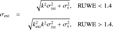
The distribution of Δϖ normalized by its total or external uncertainty σext should have a mean of zero and a standard deviation of one. The external uncertainty was calculated as follows:
 (3)
(3)
where σint is the internal (catalog) random uncertainty, σs is the systematic uncertainty, and k is a multiplicative constant that needs to be determined and that may depend on magnitude or other quantities. The value obtained for σs in Paper I was 10.3 μas and that is the value that is used here. For further details on the definitions, see Paper I.
In this Paper I present new estimations of the Gaia EDR3 parallax bias and of k based on the analysis of the parallaxes of stars that belong to open clusters (from Villafranca I and II), globular clusters (from Paper I), and from the Large Magellanic Cloud (LMC) and the Small Magellanic Cloud (SMC) (from Luri et al. 2021). The new ZEDR3 relies on the absolute QSO zero point of L21b but is otherwise independent of their calculation. The new estimations are applicable only to stars with five-parameter astrometric solutions in the case of ZEDR3 but for k I extend the analysis to six-parameter astrometric solutions. In the next section I describe the data and methods and in the following one I present and analyze the results. I conclude with a summary and possible ways to expand this work.
2 Data and methods
2.1 How the sample was selected
As mentioned above, the sample in this paper is a combination of stars with good-quality Gaia EDR3 data from four types of objects: the LMC, the SMC, globular clusters, and open clusters. I first describe the selection process for the Magellanic Clouds and then I do it for the stellar clusters.
For the LMC and the SMC I start with the sample obtained by Luri et al. (2021), who used an iterative procedure to eliminate nonmembers. I then restrict the sample to those objects [a] within 10° of the respective galaxy centers, [b] with RUWE < 1.4 (Renormalized Unit Weight Error, see L21a), [c] with five-parameter Gaia EDR3 solutions (see L21a), and [d] with σext < 100 μas using the k and σs values from Paper I. This leaves us with a total of 989 909 LMC stars and 196 413 SMC stars with good-quality Gaia EDR3 parallaxes. As there are few stars fainter than G = 18 mag among those and because of the way the rest of the sample is selected, I add the additional condition [e] with G < 18 mag, leaving us with 950 696 LMC stars and 192 266 SMC stars.
For the globular clusters I use the sample from Paper I that consists of stars from six such systems (ω Cen, 47 Tuc, NGC 6752, M5, NGC 6397, and M13). The selection of the stars was performed applying the same [b] to [e] conditions as in the previous paragraph, with the total number of stars for the six globular clusters being 30 577, ranging from the 1154 in M5 to the 14 606 in 47 Tuc (I note that Table 5 in Paper I includes stars with six-parameter solutions, which are excluded here). The sample in each cluster is selected by position and proper motion and applying a 4σ cut in normalized parallax (see Paper I for details). The selection technique can be described as a simplified version as the one used by Luri et al. (2021), as globular clusters are more simple systems than the MCs and are also located at closer distances, which makes it easier to eliminate contaminants.
The sample for the open clusters1 consists of stars from 26 such systems, named as Villafranca O-001 to Villafranca O-026. The first sixteen of those were originally defined in Villafranca I and the next ten were added in Maíz Apellániz et al. (2022). In that second paper the main criterion for adding OB groups to the list was precisely their usefulness for the analysis here, namely, the addition of a large number of stars per cluster with a high degree of certainty in membership. The sixteen Villafranca I OB groups were originally analyzed with Gaia DR2 astrometry but they were re-analyzed with Gaia EDR3 astrometry (together with the ten new groups) in Villafranca II. For the North America nebula I use Villafranca O-014 NW as the cluster. The selection process of the sample in each open cluster is the same as that in Villafranca I and II and is similar to that of the globular clusters with two general differences: an additional cut using a displaced isochrone in the CMD is applied and the cut in normalized parallax is applied at 3σ instead of at 4σ. The reason behind the first difference is that OB groups are usually located close to the Galactic plane, where the field population is a stronger contaminant than for globular clusters. The second difference arises from the lower number of stars selected per cluster, which ranges from 11 (Villafranca O-013) to 482 (Villafranca O-022), for a total of 3155 stars in open clusters (I note that the numbers in Villafranca I are from Gaia DR2, not Gaia EDR3, and that the statistics in both Villafranca papers also include stars with six-parameter solutions). Additionally, eleven stars that satisfied all requirements except that of the normalized parallax were added by hand because they are bright stars that were excluded by a small margin and additional information suggests they are indeed cluster members. As we see below, their original exclusion was caused by the underestimation of k for bright stars in Paper I. The eleven stars are listed in Table 1.
Stars in open clusters manually added to the sample.
2.2 Why the sample was selected
The first goal in this paper is to derive a new parallax zero point for the five-parameter solutions in Gaia EDR3 following the same parameter dependencies of L21b, that is:
 (4)
(4)
with the different terms explained in Appendix A of L21b and Sect. 2 of Paper I. In summary, there are eight possible terms for a given magnitude G: q00, q01, q02 are the three color-independent β terms; q10, q20, q30, and q40 are the three β-independent color terms (with the first one applying to the intermediate color range where most stars are located, the next two to red stars, and the last one to blue stars); and q11 is the only term that depends on both color and β. Ideally, one should cover the G+νeff+β ranges of interest as thoroughly and uniformly as possible. In practice this is not possible for a number of reasons:
-
In general, faint stars are more common than bright ones.
-
Single-age populations follow quasi-one-dimensional distributions (isochrones) in a CMD.
-
Stars are not uniformly distributed over the whole sky.
-
The presence of contaminants should be minimized.
The approach in this paper is to use the four different samples described above to try to cover the three-dimensional space of interest as best as possible. To describe how that is done, I divide G in three ranges: faint(13 < G < 18), intermediate (9.2 < G < 13), and bright (6 < G < 9.2) and use Figs. 1–3 to analyze how our sample is distributed.
The faint range is the better covered, as the LMC and SMC include objects of most magnitudes and colors and the small gaps left are well complemented with the other two samples. The issue with the LMC and SMC is that they are both located near the south ecliptic pole, so clusters are needed to extend the solution to other latitudes (Fig. 3).
In the intermediate range the coverage is not as good and here is where the presence of different types of samples becomes even more useful. For the fainter end of the range the MCs are still the dominant contribution but only forblue and red colors, not intermediate ones. As we move to brighter magnitudes in this range, globular clusters become the most common population but only for red stars. Finally, for objects brighter than G = 10 mag open clusters dominate but most of them are blue.
The worst coverage of all is for bright stars. The sample is very small and it is composed almost exclusively of blue stars in open clusters.
In summary, I expect ZEDR3 to be better characterized for faint stars than for bright ones. However, I emphasize one important point of the technique employed in this paper. Cluster (or galaxy) memberships are determined simultaneously for stars of very different magnitudes and colors and, given the behavior of the parallax uncertainties as a function of magnitude, the largest weight in determining the distance (and, hence, establishing membership) is given to faint stars with 13 < G < 16 for most systems. Therefore, stars in the intermediate and bright ranges are anchored with respect to the better characterized faint stars. The reason for not doing a separate analysis for six-parameter solutions at this stage is that the sample of such stars in the intermediate and faint ranges is small (Fig. 12 in L21b) but see below for the value of k.
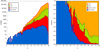 |
Fig. 1 Left: G magnitude histogram for the samples in this paper using 0.2 mag bins and with a logarithmic vertical scale. I note that the distribution of each sample is plotted above that of the following one, so the top line should be interpreted as the histogram for the total sample. Right: fraction that each sample contributes per 0.2 mag bin. |
2.3 What was done with the sample
For the stars in the 26 open clusters, six globular clusters, the LMC, and the SMC I used Eq. (1) with the ZEDR3 from L21b (ZEDR3,Lin) to calculatethe group parallaxes and applied Eq. (2) to obtain ΔϖLin for each star. I note that in the case of the LMC and SMC I use the measured group parallax as a reference, not the expected value from external measurements, which is within one sigma of the uncertainty (including the angular covariance terms) but off by a few μas (Paper I). In this way, the analysis in this paper deals with the behavior of ZEDR3 as a function of magnitude, color, and ecliptic latitude but does not change the global anchoring of the parallaxes with respect to the QSO values or studies the effect of the angular covariance for small or intermediate angles.
As previously mentioned, when normalized by its uncertainty, Δϖ should have a mean of zero and a standard deviation of one. As discussed in the next section, I detected that is not the case for the combination of ΔϖLin and the internal uncertainties: the standard deviation is larger than one for all magnitudes and the mean is very close to one for G > 13 but deviates in some cases for brighter stars. The first effect means that k is significantly different from one (even after accounting for the effect of σs in Eq. (3)) and the second one that it is possible to improve ZEDR3,Lin for bright stars. Both of those effects were anticipated in Paper I and are corroborated here. Therefore, after the test using ZEDR3,Lin I derive and test an alternative zero point in the next section.
3 Results
In this section I first describe the behavior of ΔϖLin as a function of magnitude, color, and ecliptic latitude in terms of its average,  , and (non-normalized) standard deviation, σΔϖ for the L21b zero point. I then explain how the new zero point is calculated. Finally, I compare the two results.
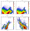 |
Fig. 2 CMDs for the LMC (upper left), SMC (upper right), globular cluster (lower left), and open cluster (lower right) samples. The intensity scale is logarithmic and the cell sizes are 0.01 μm−1 × 0.1 mag (upper panels) and 0.02 μm−1 × 0.2 mag (lower panels). The color bars at the right of each plot give the number of stars per cell, I note that they are very different from panel to panel. The upper x axes use Eq. (4) of L21a to transform from νeff to GBP − GRP. |
3.1 The Lindegren zero point
One problem with analyzing data that depends on three parameters (in this case, G, νeff, and β) is how to display them. Given the characteristics of the data, I do it in in multiple ways2:
- 1.
Figure 4 plots ΔϖLin as a function of G for the whole sample, as that is the parameter that most influences the quality of the parallaxes (to first order, the internal uncertainty is a function of G). In that figure I also show
 , σΔϖ, and the average (internal) parallax uncertainty as a function of G using error bars (left panel) and lines (right panel).
 - 2.
The green line in Fig. 5 plots the k value derived from the results plotted in Fig. 4 using Eq. (3) and assuming that σΔϖ is the external uncertainty.
- 3.
The left panel of Fig. 6 displays a 2D histogram of
 as a function of G and νeff (i.e., a CMD) and in Table 2 the values of a simplified version of the histogram together with the values of σΔϖ and k are given.
 - 4.
The inclusion of the effect of the ecliptic latitude is more difficult to visualize because most of the sample is either from the LMC (80.8%), located around the south ecliptic pole, or the SMC (16.3%), not too far from it. On the other hand, the remaining sample (clusters, 2.9%) is more uniformly distributed over the celestial sphere (Fig. 3). Therefore, to compare the effect between a sample that changes litlle in β with one that is more distributed, I use Figs. 6 and 7, keeping in mind Fig. 2 to remember in which areas of the CMD the LMC and SMC population are not dominant.
- 5.
To visualize the fitted functions themselves, I use Fig. 8, which is inspired on Fig. 20 of L21b but with two differences: the full functions are plotted (as opposed to individual points) and three panels are used for each fit to show the changes induced by β. In that respect, I note that q00, q01, and q02 shift the different G sections up and down between panels but do not change the overall aspect of the plot. That is caused by q11 the mixed color-latitude term and that is why the largest difference between the three left plots in Fig. 8 takes place around G = 12, as that is the magnitude at which the q11 in ZEDR3,Lin is larger in the G = 6−18 range.
I analyze the L21b zero point using the same three magnitude ranges previously described: faint (13 < G < 18), intermediate (9.2 < G < 13), and bright (6 < G < 9.2).
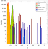 |
Fig. 3 β (ecliptic latitude) histogram for the samples in this paper using 1° bins and with a logarithmic vertical scale. I note that the distribution of each sample is plotted above that of the following one, so the top line should be interpreted as the histogram for the total sample. |
3.1.1 Faint range: 13 < G < 18
With some minor exceptions, the L21b zero point works very well in the faint magnitude range.  stays close to zero for all magnitudes in Fig. 4 and that is reflected in the first relevant column of Table 2, where all absolute values of
  are less than 1 μas for G > 13.5 and ~ 2 μas in the G = 13.0−13.5 range. Equivalently, mosts cells in the left panel of Fig. 6 for G > 13. The only significant local effect in Fig. 4 is caused by the concentration of sources around G = 13.8 (red clump stars in the relatively metal-rich globular cluster 47 Tuc), but that is just an effect of a few μas. In the left panels of Figs. 6 and 7 (especially in the second case), I see a larger effect: for both very blue stars (mostly extreme horizontal branch stars in globular clusters) and very red stars with G > 16,
  is < −40 μas in Fig. 7 and shows negative values in Fig. 6, with the caveat that the number of stars per cell is small. That is the one of the few CMD regions where the L21b zero point might be improved in the faint range.
3.1.2 Intermediate range: 9.2 < G < 13
The situation is different in the intermediate range. For 11 < G < 13,  is consistently negative in Fig. 4 and in the first group of columns in Table 2, with indication of substructures as a function of G at least for 12 < G < 13 and possibly also for 11 < G < 12. The two additional
  columns in Table 2 and the left panel of Fig. 6 reveal that the deviations are significantly larger for blue stars, with a value of almost − 17 μas for the 242 stars with 11.5 < G < 12.0 and νeff > 1.5 μm−1. This effect was already hinted at by L21b (their Sect. 6.2) in the LMC data but could not be better checked by them due to the absence of a larger sample. For 9.2 < G < 11,
  is also negative for blue stars (but by a smaller amount than for 11 < G < 12) but for red stars it is positive (with a smaller sample). Therefore, the L21b zero point can be significantly improved in this range.
3.1.3 Bright range: 6 < G < 9.2
In this range the number of stars is smaller, so the analysis of the L21b zero point cannot be as thorough. Two main issues can be described. First, σΔϖ increases significantly, with a large effect on k (see below). Second,  has the largest deviations from zero of all ranges, following a sequence of negative-positive-negative values as one progresses toward brighter magnitudes. However, those aspects have to be qualified by the small sample and by almost all bright stars in the sample being blue. It is possible to improve the L21b zero point in this range but being subject to larger uncertainties in the outcome.
3.1.4 The k multiplicative constant
The behavior of k in Fig. 5 for L21b has a qualitative similar one to the approximation derived in Paper I for G > 10. An increase from ~1.1 at G = 18 as we move toward G ~ 12 followed by a decrease as we move toward G = 10. However, some (relatively small) differences are seen in that range, not surprising given the better sampling of the data here: the peak around G ~ 12 is taller, wider, and has some structure. The situation is very different for G < 10, a range that was not probed in Paper I. Starting around G = 10, where k ~ 1.3, it grows to values close to 2.0 around G = 9 and close to 3.0 for the brightest stars sampled here. Pending the derivation of the new zero point below, I defer until then the analysis of the consequences of this effect.
3.2 Calculating the new zero point
As just described, the Lindegren zero point works reasonably well for most values of its parameters, G, νeff, and β, but can be tweaked in some circumstances. Based on that, I define the new zero point as the sum of the Lindegren one and a correction term:
 (5)
(5)
The goal is to derive the optimal ΔZEDR3 by fitting ΔϖLin to obtain ZEDR3,new. This strategy works because the zero point is the sum of a series of linear terms. The decomposition into two terms has several advantages. First, it allows us to characterize the impact of the correction better. Second, I can fit just a selection of the whole set of coefficients, leaving the ones from L21b that do not require changes to be left in place. And third, it allows the anchoring of the parallaxes to remain unchanged, as previously mentioned.
To calculate ΔZEDR3 I assumed the same functional form as L21b and added three magnitude breakpoints (knots) at G = 7.4, 9.2, and 18.0. The last oneis added because it is the end of the magnitude range in our sample. The first two are added based on Fig. 4, as the behavior of Δϖ in G there is not linear in the G = 6.0–10.8 range and those are the apparent magnitudes at which the behavior changes (but see below for the restrictions placed on the fitted coefficients in that range).
To fit ΔZEDR3 I wrote a program in IDL based on the MPFIT package (Markwardt 2009)3. MPFIT allows for arbitrary functions to be fitted to almost any type of data while fixing the value of some coefficients and tying up others among them. As L21b correctly cautions, it is important to avoid overfitting. Therefore, initially I only fitted the coefficients where enough data were present and, by trial and error, I added additional restrictions. In the end, the following coefficients for ΔZEDR3 were fit:
For the three breakpoints at G = 6.0, 7.4, and 9.2, only q00 was fit at each one of them.q30 was not fit (as there are no stars as red as needed, see below) and the rest of the coefficients were tied up, that is, forced to have the same values at the three breakpoints.For q11 the range of bright magnitudes where the coefficients are tied up was extended to G = 10.8 and for q20 to G = 10.8, 11.2, and 11.8.
The mixed latitude-color term, q11, was also tied up in three additional regions: (a) G = 11.2 and 11.8, (b) G = 12.2 and 12.9, and (c) G = 16.1, 17.5, and 18.0.
The cubic term for red stars, q20 was tied up for G at 17.5 and 18.0.
As there are few very red stars in the sample, q30 was only fit in the G = 13.1–17.5 range and even there, the two values at 13.1 and 15.9 were tied up and the same was done for the two values at 16.1 and 17.5.
The fitted coefficents for ΔZEDR3 are given inTable 3. The last two columns give the combinations of the first five coefficients at the south ecliptic pole, which is a reasonable approximation for the LMC stars. The final ZEDR3,new is given in Table 4, where for magnitudes fainter than G = 18.0 the values given are simply those of ZEDR3,Lin, as the sample in this paper does not reach those very faint magnitudes. The values of the new zero point are plotted in the right column of Fig. 8, allowing for a direct comparison with the L21b zero point. To facilitate the implementation of the new results, two IDL routines are given in Tables A.1 and A.2. The first one produces the k multiplicative constant and the second one the new zero point.
As a final note, I am fitting ΔϖLin to obtain a new ΔZEDR3 and the values of ΔϖLin depend on the group parallaxes calculated with the L21b zero point. In principle, one could iterate the process by using the new group parallaxes obtained with ZEDR3,new (i.e., the ones that are listed in Villafranca II for the open clusters) and calculate a new incremental zero point to be added to the previous one. However, that was found unnecesary because the differences between the old and new group parallaxes are small (~ 1 μas) and unbiased (some positive and some negative), leading to very similar values of ZEDR3,new.
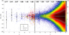 |
Fig. 4 Residuals using the Lindegren zero point, ΔϖLin, as a functionof G. The plotis divided into two panels due to the differences in the sample sizes for stars with G between 6 and 12 mag (left panel) and stars with G between 12 and 18 mag (right panel). In the left panel all stars are plotted individually with a color+symbol code used to differentiate between the four samples used in this paper. In the right panel the stellar density is plotted combining all objects and using a logarithmic color scale, with the bar at the left indicating the number of objects in each 0.02 mag × 2 μas cell. The black points in the left panel show the average ΔϖLin in each magnitude bin. The error bars show the average of the parallax uncertainties (small values) and the dispersion of ΔϖLin (large values), also in each magnitude bin. In the right panel the points and error bars are substituted by lines displaying the same information. The text at the top of the panels gives the value of k in each magnitude bin as determined from the dispersion of ΔϖLin and the average parallax uncertainty. |
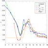 |
Fig. 5 k as a function of magnitude for all colors using the Lindegren zero point (Table 2) and for the three cases in Table 5 using the results in this paper. The data points are calculated at 1 mag intervals for G < 10 and at 0.5 mag intervals for G > 10 and joined by a spline. The orange line shows the approximation derived in Paper 1. |
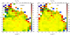 |
Fig. 6 Average residual as a function of νeff and G using the Lindegren zero point (left) and the one proposed here (right) for the full sample. The left bar shows the scale in μas. Each cell hasa size of 0.05 μm−1 × 0.5 mag. Cells with less than ten objects used to calculate the average include the number of objects. The color scale is capped for values above 60 μas or below −60 μas for display purposes but some cells (seven in the left panel, and four in the right panel) are outside that range. The upper x axes use Eq. (4) of L21a to transform from νeff to GBP − GRP. |
Statistics (in μas) by G magnitude and νeff ranges using the Lindegren correction.
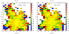 |
Fig. 7 Same as Fig. 6, but using only the cluster sample. Here the number of cells outside the range is 17 in the left panel and 16 in the right panel. |
ΔZEDR3(G, νeff, β) coefficients for 5-parameter solutions calculated in this paper.
3.3 Analysis
I now analyze ZEDR3,new by using it to calculate the new group parallaxes and studying the residuals using the new zero point, Δϖnew. For that purpose I use Fig. 9, the equivalent to Fig. 4, Table 5, the equivalent to Table 2, and the already introduced Figs. 5–8 and Tables 3 and 4. As I did for the Lindegren zero point, I divide the analysis in the same three magnitude ranges.
3.3.1 Faint range: 13 < G < 18
As expected, the differences between the Lindegren and the new zero points are small for most values of the parameter space for faint stars. This is especially true near the south ecliptic pole (in our sample, the LMC and SMC), as evidenced by the small values in the last two columns of Table 3 and the similar appearance of the top two panels in Fig. 8 for G > 13. However, in some cases the differences are significant:
The largest one is the existence of a relatively large ΔZEDR3 mixed color-latitude term (q11) for G > 16.1. While the top two plots of Fig. 8 are similar for those magnitudes, the bottom two plots are quite different.
The new zero point also has a significant q40 term (blue stars) in this magnitude range, as established with the help of extreme horizontal branch stars in globular clusters. Δϖnew is smaller than ΔϖLin for them (bottom left corner of both panels in Fig. 7, the effect is also seen to some degree in Fig. 6). However, some residuals are still seen, especially for stars bluer than νeff = 1.8 μm−1. At this stage it is not clear whether the effect is caused by small number statistics or by the need of using a different functional form for the zero point (e.g., a q41 term), but I note that the effect is also seen in the bottom two panels of Fig. 10 in L21b.
L21b detected the existence of a “hook” in the behavior of the reddest stars (νeff < 1.18 μm−1) for G > 16. The effect is also seen in the bottom right corners of Figs. 6 and 7 but as the functional form does not include a term there, the new zero point does not correct for it and the appearance does not change significantly between the left and right panels.
Nevertheless, we should bear in mind that for most stars in this magnitude range the effect is small. In that way, Figs 4 and 9 are very similar for G > 13. Doing a more quantitative comparison, nine out of the thirty values of  in Table 2 have absolute values larger than 1 μas, a number that in Table 5 is reduced to five (very good statistics if one bears in mind that σs = 10.3 μas). In summary, for 13 < G < 16 the new zero point is very similar to the Lindegren zero point and for 16 < G < 18 some differences appear for stars far from the south ecliptic pole and for very blue and very red stars.
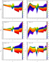 |
Fig. 8 ZEDR3 as a function of G (horizontal axes) and νeff (color bar) for the L21b zero point (left column) and the new zero point in this paper (right column). The black lines correspond to the values of the nine ticks in the color bar. To visualize the β effect, each ZEDR3 is evaluated atthe ecliptic south pole (top panels), equator (middle panels), and north pole (bottom panels). I note that for G < 12.9 ZEDR3 has no color dependence in the νeff = 1.1−1.24 μm−1 range, as q30 = 0. Breakpoints are marked with vertical dotted lines. Compare with the top panel in Fig. 20 of L21b. |
ZEDR3,new(G, νeff, β) coefficients for 5-parameter solutions calculated from L21b and the results in this paper.
Statistics (in μas) by G magnitude and νeff ranges using the results in this paper.
3.3.2 Intermediate range: 9.2 < G < 13
The new zero point is significantly different from the Lindegren one for intermediate magnitudes, even for positions close to the south ecliptic pole (Fig. 8). For β = −90°, ZEDR3,new is qualitatively similar to ZEDR3,Lin (with a reversal of the behavior as a function of color with respect to fainter magnitudes in both cases) but quantitatively different for 11 < G < 13. For brighter stars (continuing to G = 6) a large q40 term appears, making ZEDR3,new more negative for blue stars. As for the changes as a function of β, they are small for 11 < G < 12 and significant otherwise.
Analyzing the  values in Table 2 for 9 < G < 13 I find just six out of twenty one with absolute values smaller than 2 μas and five with absolute values largerthan 5 μas. On the other hand, in Table 5 thirteen out of twenty one values have absolute values smaller than 2 μas and there are none above 5 μas. It is clear that the new zero point lowers the residuals and provides a better fit. The effect is also seen in the comparison between Figs. 4 and 9, especially for 11 < G < 13. I note the apparent existence of some fine structure as a function of G with an amplitude of a few μas for at least 12 < G < 13 that could be further corrected in the future by introducing additional magnitude breakpoints.
The improvement is not the same for all magnitudes and colors. From Tables 2 and 5 and Figs. 6 and 7, we see that it is larger for blue stars than for red ones and for 11 < G < 12 than for other magnitudes in this range. The main shortcoming of the new zero point arises from the relatively small sample size, especially for the brighter part of the magnitude range for red stars. One possible improvement in this sense would be to add open clusters with red supergiants to the analysis. In summary, for 9.2 < G < 13 the new zero point provides a significant improvement with respect to the Lindegren zero point.
3.3.3 Bright range: 6 < G < 9.2
Once we get to this magnitude range, the sample is highly incomplete and consists almost exclusively of blue stars. ΔZEDR3 has large q00 and (as already mentioned) q40 terms, leading to significant changes in the overall zero point and on its color dependence for blue stars (Fig. 8). ZEDR3,new is capable of partially flattening the behavior of  in Fig. 9 and Table 5 with respect to Fig. 4 and Table 2. Still, the values are not zero and the most visible characteristic is the persistence of the large values of σΔϖ, which in turn lead to the same effect for k, as we see in the next subsection. In summary, for bright stars the new zero point improves upon the Lindegren zero point but provides little information for red stars and this magnitude range is dominated by the effect of the large dispersion of the results, indicating a significant underestimation of the external parallax uncertainties by the internal values.
3.3.4 The k multiplicative constant
Table 5 lists the values of k as a function of magnitude using the new zero point, including all colors in the calculation or just the blue or the red stars. The values are also plotted in Fig. 5 and can be compared with the results form the Lindegren zero point in Table 2 and in the same figure. For faint stars the results for both zero points are identical, an indication of the similarity between the two zero points in that magnitude range. For intermediate and bright stars the new zero point reduces the value of k but only slightly so. This must be interpreted as the effect of ΔZEDR3, the transformation from the Lindegren zero point to the new one (the correction of a systematic effect), being in general small compared to the true random uncertainties. The ultimate reason why we can measure ΔZEDR3 is because we are using large numbers of stars in each cluster or galaxy. On the other hand, the introduction of the k value (and, to a lesser extent, of σs) in the transformation of internal uncertainties to external ones is an important effect, given that it is significantly larger than one.
The comparison between blue and red stars in Table 5 shows a similar behavior as a function of G, indicating that a singlek(G) is a good approximation. Nevertheless, there are some differences. For most magnitudes k appears to be slightly lower for red stars. The exception is the region around G ≈ 12.7, where the local maximum in k for red stars is located. The equivalent maximum for blue stars is located around G ≈ 11.3.
The largest values of k occur for bright stars (G < 9.2) and that is the single most important conclusion of this work: using the internal uncertainties leads to a significant undestimation of their Gaia EDR3 distance uncertainties. The effect is also important for stars with 11 < G < 13. An example of the effect is seen in the case of the eleven intermediate/bright stars listed in Table 1: all of their Gaia EDR3 parallaxes are within 3 sigmas of the group values if one uses the k(G) in Table 5.
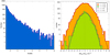 |
Fig. 10 Left:RUWE histogram of five-parameter sources from the 32 stellar clusters in our sample used to evaluate kext. Right: normalized parallax histograms for faint and bright sources with RUWE between 1.4 and 8.0. The two fits correspond to values of kext of 2.36 and 1.88, respectively. |
3.3.5 Objects with large RUWE
The results presented so far refer to objects with five-parameter solutions and “good” RUWE, that is, values up to 1.4. However, as shown in Paper I, it is possible to treat objects with RUWE larger than 1.4 by introducing an additional factor, kext, in Eq. (3) multiplying σint, that is:
 (6)
(6)
Here I present an extended analysis of this issue.
I select the five-parameter solutions in each of the 32 clusters in our sample with [a] G between 6 and 18, [b] RUWE between 1.4 and 8.0, [c] no restrictions on parallax uncertainty, and [d] the rest of the restrictions that apply to each individual cluster. I apply ZEDR3,new and subtract the group parallax to each individual parallax value to calculate Δϖnew and I use Eq. (3) to obtain σext,0, that is, the external uncertainty assuming the same k as for objects with RUWE lower than 1.4. Finally, I make a 9-sigma cut in normalized parallax, the value being so high because we expect the real external uncertainties to be larger than for objects with good RUWE. The final sample has 6227 objects.
The distributions of RUWE and of normalized Δϖnew are shown in Fig. 10. I divide the sample in a faint and a bright range (limited by G = 14) and calculate Gaussian fits with zero mean. The results are excellent, indicating that parallaxes with large RUWE are not strongly biased toward higher or lower values and that the inclusion of a kext results in external uncertainties with the proper behavior. kext is significantly larger for fainter stars, leading us to divide G in bins to tabulate its behavior. Unfortunately, there are few bright stars in this sample, so the information there is limited and a single bin for the G = 6–13 has to be used. The results are given in Table 6 and have been incorporated into Table A.1.
3.3.6 Objects with six-parameter astrometric solutions
As previously mentioned, there are not enough stars with six-parameter solutions to derive a new ZEDR3 for them. However, as we have seen, the value of k is relatively robust with respect to the zero point and can be calculated even with a relatively small number of points. In the case of our cluster sample, we have enough stars to determine it for the range 13 < G < 18. The values of k for six-parameter solutions there follow the same pattern as in Fig. 5 for five-parameter solutions, growing from G ~ 18 to G ~ 13 but with values that are ~ 1.25 times higher. Therefore, a simple approximation is to use a value of kext of 1.25 for six-parameter solutions, that is:
 (7)
(7)
but I note that it is not tested for G < 13. That approximation has been incorporated into Table A.1.
kext calculated in magnitude bins for five-parameter solutions using the stellar cluster data for objects with RUWE between 1.4 and 8.0.
4 Summary and future work
In this paper I have presented a new zero point for Gaia EDR3 parallaxes as a function of magnitude, color, and ecliptic latitude. I have used the same functional form as L21b (Eq. (4)) but derived the zero point using a combination of data from the LMC, the SMC, globular clusters, and open clusters. The differences between the two zero points are small for faint stars (G > 13) but become significant for stars brighter than that, though it should be noted that for G < 9.2 the zero point is poorly defined due to the small size of the sample. As a second result, I have determined that the multiplicative constant k that is used to convert from internal parallax uncertainties to external ones (Eq. (3)) is significantly larger than one for most stars and even larger than two for G < 9.2. k is found to be even larger for objects with RUWE larger than 1.4 or with six-parameter solutions. Therefore, the distance uncertainties derived assuming internal parallax uncertainties will be, in general, underestimated.
Gaia DR4 is stil several years in the future and this paper has not exploited all of the possibilities for improving on the zero point. The most obvious future line of work would be adding more clusters to improve the statistics for bright stars. It would be especially interesting to include young clusters with red supergiants, as those would extend the sampling to a larger range of colors (bright red stars) and of ecliptic latitudes. Red giants in additional globular clusters would also help but to a lesser degree regarding bright red stars, given that the tip of the red giant branch (TRGB) is not too bright (bottom left panel in Fig. 2) and that there are only a few nearby globular clusters. However, adding globular clusters would be helpful in calibrating two regions of the CMD: RGB stars for the intermediate/faint very red region (the dominant Gaia population in some regions of the Galactic plane lies there in the form of high-extinction red giants) and blue horizontal branch (BHB) stars for the faint very blue region. The latter could be used to test whether the residuals for very blue stars described in Sect. 3.3.1 could be corrected with a latitude dependence. Other possibilities would be testing new basis functions and magnitude breakpoints and building a sample large enough to test the zero point for six-parameter solutions. Once Gaia DR4 becomes available, these same clusters could be used to determine its (hopefully smaller) parallax zero points.
Acknowledgements
I acknowledge support from the Spanish Government Ministerio de Ciencia through grant PGC2018-095 049-B-C22. This work has made use of data from the European Space Agency (ESA) mission Gaia4, processed by the Gaia Data Processing and Analysis Consortium (DPAC5). Funding for the DPAC has been provided by national institutions, in particular the institutions participating in the Gaia Multilateral Agreement. The Gaia data is processed with the computer resources at Mare Nostrum and the technical support provided by BSC-CNS.
Appendix A IDL codes
Function that calculates Gaia EDR3 parallax external uncertainties.
Function that calculates the Gaia EDR3 zero point for an array of values.
References
- Brown, A. G. A., Vallenari, A., Prusti, T., et al. 2021, A&A, 649, A1 [NASA ADS] [CrossRef] [EDP Sciences] [Google Scholar]
- Campillay, A. R., Arias, J. I., Barbá, R. H., et al. 2019, MNRAS, 484, 2137 [Google Scholar]
- Lindegren, L., Klioner, S. A., Hernández, J., et al. 2021a, A&A, 649, A2 [EDP Sciences] [Google Scholar]
- Lindegren, L., Bastian, U., Biermann, M., et al. 2021b, A&A, 649, A4 [EDP Sciences] [Google Scholar]
- Luri, X., Chemin, L., Clementini, G., et al. 2021, A&A, 649, A7 [NASA ADS] [CrossRef] [EDP Sciences] [Google Scholar]
- Maíz Apellániz, J. 2019, A&A, 630, A119 [NASA ADS] [CrossRef] [EDP Sciences] [Google Scholar]
- Maíz Apellániz, J., Crespo Bellido, P., Barbá, R. H., Fernández Aranda, R., & Sota, A. 2020, A&A, 643, A138 (Villafranca I) [NASA ADS] [CrossRef] [EDP Sciences] [Google Scholar]
- Maíz Apellániz, J., Pantaleoni González, M., & Barbá, R. H. 2021, A&A, 649, A13 (Paper I) [NASA ADS] [CrossRef] [EDP Sciences] [Google Scholar]
- Maíz Apellániz, J., Barbá, R. H., Fernández Aranda, R., et al. 2022, A&A, 657, A131 [NASA ADS] [CrossRef] [EDP Sciences] [Google Scholar]
- Markwardt, C. B. 2009, ASP Conf. Ser., 411, 251 [Google Scholar]
I use the term “open cluster” to refer to the OB groups defined in Villafranca I and II even though some of them are not strictly bound systems. However, for the purposes of this paper that is irrelevant, as their spread in distances introduces a dispersion in their parallaxes that is small in comparison with the effects I am trying to measure.
Available from http://purl.com/net/mpfit
All Tables
Statistics (in μas) by G magnitude and νeff ranges using the Lindegren correction.
ΔZEDR3(G, νeff, β) coefficients for 5-parameter solutions calculated in this paper.
ZEDR3,new(G, νeff, β) coefficients for 5-parameter solutions calculated from L21b and the results in this paper.
Statistics (in μas) by G magnitude and νeff ranges using the results in this paper.
kext calculated in magnitude bins for five-parameter solutions using the stellar cluster data for objects with RUWE between 1.4 and 8.0.
All Figures
|
Fig. 1 Left: G magnitude histogram for the samples in this paper using 0.2 mag bins and with a logarithmic vertical scale. I note that the distribution of each sample is plotted above that of the following one, so the top line should be interpreted as the histogram for the total sample. Right: fraction that each sample contributes per 0.2 mag bin. |
| In the text | |
|
Fig. 2 CMDs for the LMC (upper left), SMC (upper right), globular cluster (lower left), and open cluster (lower right) samples. The intensity scale is logarithmic and the cell sizes are 0.01 μm−1 × 0.1 mag (upper panels) and 0.02 μm−1 × 0.2 mag (lower panels). The color bars at the right of each plot give the number of stars per cell, I note that they are very different from panel to panel. The upper x axes use Eq. (4) of L21a to transform from νeff to GBP − GRP. |
| In the text | |
|
Fig. 3 β (ecliptic latitude) histogram for the samples in this paper using 1° bins and with a logarithmic vertical scale. I note that the distribution of each sample is plotted above that of the following one, so the top line should be interpreted as the histogram for the total sample. |
| In the text | |
|
Fig. 4 Residuals using the Lindegren zero point, ΔϖLin, as a functionof G. The plotis divided into two panels due to the differences in the sample sizes for stars with G between 6 and 12 mag (left panel) and stars with G between 12 and 18 mag (right panel). In the left panel all stars are plotted individually with a color+symbol code used to differentiate between the four samples used in this paper. In the right panel the stellar density is plotted combining all objects and using a logarithmic color scale, with the bar at the left indicating the number of objects in each 0.02 mag × 2 μas cell. The black points in the left panel show the average ΔϖLin in each magnitude bin. The error bars show the average of the parallax uncertainties (small values) and the dispersion of ΔϖLin (large values), also in each magnitude bin. In the right panel the points and error bars are substituted by lines displaying the same information. The text at the top of the panels gives the value of k in each magnitude bin as determined from the dispersion of ΔϖLin and the average parallax uncertainty. |
| In the text | |
|
Fig. 5 k as a function of magnitude for all colors using the Lindegren zero point (Table 2) and for the three cases in Table 5 using the results in this paper. The data points are calculated at 1 mag intervals for G < 10 and at 0.5 mag intervals for G > 10 and joined by a spline. The orange line shows the approximation derived in Paper 1. |
| In the text | |
|
Fig. 6 Average residual as a function of νeff and G using the Lindegren zero point (left) and the one proposed here (right) for the full sample. The left bar shows the scale in μas. Each cell hasa size of 0.05 μm−1 × 0.5 mag. Cells with less than ten objects used to calculate the average include the number of objects. The color scale is capped for values above 60 μas or below −60 μas for display purposes but some cells (seven in the left panel, and four in the right panel) are outside that range. The upper x axes use Eq. (4) of L21a to transform from νeff to GBP − GRP. |
| In the text | |
|
Fig. 7 Same as Fig. 6, but using only the cluster sample. Here the number of cells outside the range is 17 in the left panel and 16 in the right panel. |
| In the text | |
|
Fig. 8 ZEDR3 as a function of G (horizontal axes) and νeff (color bar) for the L21b zero point (left column) and the new zero point in this paper (right column). The black lines correspond to the values of the nine ticks in the color bar. To visualize the β effect, each ZEDR3 is evaluated atthe ecliptic south pole (top panels), equator (middle panels), and north pole (bottom panels). I note that for G < 12.9 ZEDR3 has no color dependence in the νeff = 1.1−1.24 μm−1 range, as q30 = 0. Breakpoints are marked with vertical dotted lines. Compare with the top panel in Fig. 20 of L21b. |
| In the text | |
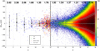 |
Fig. 9 Same as Fig. 4, but using the zero point proposed here. |
| In the text | |
|
Fig. 10 Left:RUWE histogram of five-parameter sources from the 32 stellar clusters in our sample used to evaluate kext. Right: normalized parallax histograms for faint and bright sources with RUWE between 1.4 and 8.0. The two fits correspond to values of kext of 2.36 and 1.88, respectively. |
| In the text | |
Current usage metrics show cumulative count of Article Views (full-text article views including HTML views, PDF and ePub downloads, according to the available data) and Abstracts Views on Vision4Press platform.
Data correspond to usage on the plateform after 2015. The current usage metrics is available 48-96 hours after online publication and is updated daily on week days.
Initial download of the metrics may take a while.