| Issue |
A&A
Volume 657, January 2022
|
|
|---|---|---|
| Article Number | A52 | |
| Number of page(s) | 20 | |
| Section | Planets and planetary systems | |
| DOI | https://doi.org/10.1051/0004-6361/202142196 | |
| Published online | 11 January 2022 | |
Detection of the tidal deformation of WASP-103b at 3 σ with CHEOPS★
1
Instituto de Astrofísica e Ciências do Espaço, Universidade do Porto, CAUP,
Rua das Estrelas,
4150-762
Porto,
Portugal
e-mail: This email address is being protected from spambots. You need JavaScript enabled to view it.
2
Departamento de Fisica e Astronomia, Faculdade de Ciencias, Universidade do Porto,
Rua Campo Alegre,
4169-007
Porto,
Portugal
3
IMCCE, UMR8028 CNRS, Observatoire de Paris,PSL Univ., Sorbonne Univ.,
77 av. Denfert-Rochereau,
75014
Paris,
France
4
Institute of Planetary Research, German Aerospace Center (DLR),
Rutherfordstrasse 2,
12489
Berlin,
Germany
5
Observatoire Astronomique de l’Université de Genève,
Chemin Pegasi 51,
Versoix,
Switzerland
6
Depto. de Astrofisica, Centro de Astrobiologia (CSIC-INTA), ESAC campus,
28692
Villanueva de la Cañada (Madrid),
Spain
7
Cavendish Laboratory,
JJ Thomson Avenue,
Cambridge
CB3 0HE,
UK
8
Centre for Exoplanet Science, SUPA School of Physics and Astronomy, University of St Andrews,
North Haugh,
St Andrews
KY16 9SS,
UK
9
Physikalisches Institut, University of Bern,
Gesellsschaftstrasse 6,
3012
Bern,
Switzerland
10
INAF, Osservatorio Astrofisico di Catania,
Via S. Sofia 78,
95123
Catania,
Italy
11
CFisUC, Departamento de Física, Universidade de Coimbra,
3004-516
Coimbra,
Portugal
12
Space Research Institute, Austrian Academy of Sciences,
Schmiedlstrasse 6,
8042
Graz,
Austria
13
Aix Marseille Univ, CNRS, CNES, LAM,
38 rue Frédéric Joliot-Curie,
13388
Marseille,
France
14
Center for Space and Habitability,
Gesellsschaftstrasse 6,
3012
Bern,
Switzerland
15
Astrophysics Group, Keele University,
Staffordshire
ST5 5BG,
UK
16
Department of Physics, University of Warwick,
Gibbet Hill Road,
Coventry
CV4 7AL,
UK
17
Instituto de Astrofisica de Canarias,
38200
La Laguna,
Tenerife,
Spain
18
Department of Astronomy, Stockholm University, AlbaNova University Center,
10691
Stockholm,
Sweden
19
Department of Space, Earth and Environment, Onsala Space Observatory, Chalmers University of Technology,
439 92
Onsala,
Sweden
20
Departamento de Astrofisica, Universidad de La Laguna,
38206
La Laguna,
Tenerife,
Spain
21
Institut de Ciencies de l’Espai (ICE, CSIC),
Campus UAB, Can Magrans s/n,
08193
Bellaterra,
Spain
22
Institut d’Estudis Espacials de Catalunya (IEEC),
08034
Barcelona,
Spain
23
Admatis,
5. Kandó Kálmán Street,
3534
Miskolc,
Hungary
24
Université Grenoble Alpes, CNRS, IPAG,
38000
Grenoble,
France
25
Université de Paris, Institut de physique du globe de Paris, CNRS,
75005
Paris,
France
26
Centre for Mathematical Sciences, Lund University,
Box 118,
22100
Lund,
Sweden
27
Astrobiology Research Unit, Université de Liège,
Allée du 6 Août 19C,
4000
Liège,
Belgium
28
Space sciences, Technologies and Astrophysics Research (STAR) Institute, Université de Liège,
Allée du 6 Août 19C,
4000
Liège,
Belgium
29
INAF, Osservatorio Astronomico di Padova,
Vicolo dell’Osservatorio 5,
35122
Padova,
Italy
30
Dipartimento di Fisica e Astronomia “Galileo Galilei”, Universita degli Studi di Padova,
Vicolo dell’Osservatorio 3,
35122
Padova,
Italy
31
Leiden Observatory, University of Leiden,
PO Box 9513,
2300
RA Leiden,
The Netherlands
32
Dipartimento di Fisica, Universita degli Studi di Torino,
via Pietro Giuria 1,
10125,
Torino,
Italy
33
University of Vienna, Department of Astrophysics,
Türkenschanzstrasse 17,
1180
Vienna,
Austria
34
Science and Operations Department - Science Division (SCI-SC), Directorate of Science, European Space Agency (ESA), European Space Research and Technology Centre (ESTEC),
Keplerlaan 1,
2201-AZ
Noordwijk,
The Netherlands
35
Konkoly Observatory, Research Centre for Astronomy and Earth Sciences,
1121
Budapest,
Konkoly Thege Miklós út 15-17,
Hungary
36
Sydney Institute for Astronomy, School of Physics A29, University of Sydney,
NSW
2006,
Australia
37
Institut d’astrophysique de Paris, UMR7095 CNRS, Université Pierre & Marie Curie,
98bis blvd. Arago,
75014
Paris,
France
38
ESTEC, European Space Agency,
2201AZ,
Noordwijk,
The Netherlands
39
Center for Astronomy and Astrophysics, Technical University Berlin,
Hardenberstrasse 36,
10623
Berlin,
Germany
40
Institut für Geologische Wissenschaften, Freie Universität Berlin,
12249
Berlin,
Germany
41
ELTE Eötvös Loránd University, Gothard Astrophysical Observatory,
9700
Szombathely,
Szent Imre h. u. 112,
Hungary
42
MTA-ELTE Exoplanet Research Group,
9700
Szombathely,
Szent Imre h. u. 112,
Hungary
43
Ingenieurbüro Ulmer,
Im Technologiepark 1,
15236
Frankfurt/Oder,
Germany
44
Institute of Astronomy, University of Cambridge,
Madingley Road,
Cambridge,
CB3 0HA,
UK
Received:
9
September
2021
Accepted:
15
November
2021
Abstract
Context. Ultra-short period planets undergo strong tidal interactions with their host star which lead to planet deformation and orbital tidal decay.
Aims. WASP-103b is the exoplanet with the highest expected deformation signature in its transit light curve and one of the shortest expected spiral-in times. Measuring the tidal deformation of the planet would allow us to estimate the second degree fluid Love number and gain insight into the planet’s internal structure. Moreover, measuring the tidal decay timescale would allow us to estimate the stellar tidal quality factor, which is key to constraining stellar physics.
Methods. We obtained 12 transit light curves of WASP-103b with the CHaracterising ExOplanet Satellite (CHEOPS) to estimate the tidal deformation and tidal decay of this extreme system. We modelled the high-precision CHEOPS transit light curves together with systematic instrumental noise using multi-dimensional Gaussian process regression informed by a set of instrumental parameters. To model the tidal deformation, we used a parametrisation model which allowed us to determine the second degree fluid Love number of the planet. We combined our light curves with previously observed transits of WASP-103b with the Hubble Space Telescope (HST) and Spitzer to increase the signal-to-noise of the light curve and better distinguish the minute signal expected from the planetary deformation.
Results. We estimate the radial Love number of WASP-103b to be hf = 1.59−0.53+0.45. This is the first time that the tidal deformation is directly detected (at 3 σ) from the transit light curve of an exoplanet. Combining the transit times derived from CHEOPS, HST, and Spitzer light curves with the other transit times available in the literature, we find no significant orbital period variation for WASP-103b. However, the data show a hint of an orbital period increase instead of a decrease, as is expected for tidal decay. This could be either due to a visual companion star if this star is bound, the Applegate effect, or a statistical artefact.
Conclusions. The estimated Love number of WASP-103b is similar to Jupiter’s. This will allow us to constrain the internal structure and composition of WASP-103b, which could provide clues on the inflation of hot Jupiters. Future observations with James Webb Space Telescope can better constrain the radial Love number of WASP-103b due to their high signal-to-noise and the smaller signature of limb darkening in the infrared. A longer time baseline is needed to constrain the tidal decay in this system.
Key words: planets and satellites: fundamental parameters / planets and satellites: composition / planets and satellites: interiors / planets and satellites: individual: WASP-103b / techniques: photometric / time
The transit light curves are only available at the CDS via anonymous ftp to cdsarc.u-strasbg.fr (130.79.128.5) or via http://cdsarc.u-strasbg.fr/viz-bin/cat/J/A+A/657/A52.
© ESO 2022
1 Introduction
The extreme environment that ultra-short orbital period planets are subjected to makes them ideal laboratories to study planetary physics. In addition to the very high temperatures, they also suffer from intense tidal forces which lead to a deformation of the planet’s shape (Correia & Rodríguez 2013) and shrinkage of the planet’s orbit. Hence, their study allows us to gain a wealth of information on planet-to-star tidal interactions. As part of the CHaracterising ExOplanet Satellite (CHEOPS) (Benz et al. 2021) Guaranteed Time Observing (GTO) programme, we are investigating the tidal interaction between ultra-hot Jupiters and their parent stars by attempting to measure their tidal decay and deformation.
Tidal forces tend to circularise planetary orbits and to synchronise the planetary and stellar rotation with the orbital period. In hot Jupiter systems, the orbits are usually circularised and the planet rotation is synchronised (Ogilvie & Lin 2004). However, the synchronisation of the stellar rotation is still incomplete due to the longer and still poorly unconstrained timescale of this process. Hut (1980) showed that for planets with an orbital period shorter than a third of the rotation period of the star, as it turns out tobe the case for hot Jupiters, the tidal interaction leads to the unstable transfer of angular momentum from the planetary orbit to the stellar angular momentum. This results in the planet spiralling inwards and eventually being engulfed by the star. Therefore, tidal interactions between a star and a close-in exoplanet lead to shrinkage of the orbit and eventual tidal disruption of the planet. The synchronisation timescale of the stellar rotation depends on the tidal quality factor  which is poorly constrained.
The parameter  allows us toconstrain stellar physics (e.g. Ogilvie & Lin 2007) and hence many attempts have been made to measure it. Studies of binary stars have estimated the tidal quality factor to be between 106 –107 (Meibom & Mathieu 2005). However, hot Jupiter systems could be in a different tidal regime with a higher tidal factor (
 ) and a weaker tidal decay (Ogilvie & Lin 2007; Penev & Sasselov 2011). Estimates of
  through the measurement of the orbital period decrease were successful for the following hot Jupiters: WASP-4 (
 ; Bouma et al. 2019) and WASP-12 (
 ; Maciejewski et al. 2016; Yee et al. 2020). However, the measured values of
  are lower than expected by theory (implying a stronger tidal dissipation) and it has not been possible to completely rule out other causes for the period decrease in these systems, such as apsidal precession. Statistical studies of the ensemble of known hot Jupiters show two regimes of tidal dissipation strength. The majority of the studied systems had
  , while a smaller group had
  (Collier Cameron & Jardine 2018).
The tidal deformation of a planet mostly depends on the planet-to-star distance and it is most significant for large planets that are almost filling their Roche lobe (e.g. Ferraz-Mello et al. 2008). Hence, it is larger for ultra-hot Jupiters. The radial deformationof a planet due to a perturbing potential can be quantified using the second degree fluid Love number hf (Love 1911). The Love number measures the distribution of mass within the planet depending on the concentration of heavy elements in the core of the planet relative to the envelope of the planet. Therefore, it provides insight into the internal structure differentiation of planets (Kramm et al. 2011). Correia (2014) shows that hf is proportional to an asymmetry parameter q which relates the three axes (r1, r2, and r3) of the planetary ellipsoidal shape – if r1 = r2(1 + 3q) and r3 = r2(1 − q), then
 (1)
(1)
with the volumetric radius ![Mathematical equation: $R_{\textrm{V}} =\sqrt[3]{r_1r_2r_3}{\;} M_{\textrm{p}}$](/articles/aa/full_html/2022/01/aa42196-21/aa42196-21-eq12.png) and M⋆ being the planetary and the stellar mass, respectively, R* being the stellar radius, and a being the semi-major axis of the planet’s orbit. Correia (2014) also shows that the non-spherical shape of a deformed planet along with its varying projected area during a transit modifies the transit light curve and causes anomalies in the ingress, egress, and mid-transit phases compared to a spherical case (Fig. A.1 of Correia 2014). Detecting the deformation-induced signature in the light curve can therefore allow for the measurement of the Love number (Akinsanmi et al. 2019; Hellard et al. 2019).
and M⋆ being the planetary and the stellar mass, respectively, R* being the stellar radius, and a being the semi-major axis of the planet’s orbit. Correia (2014) also shows that the non-spherical shape of a deformed planet along with its varying projected area during a transit modifies the transit light curve and causes anomalies in the ingress, egress, and mid-transit phases compared to a spherical case (Fig. A.1 of Correia 2014). Detecting the deformation-induced signature in the light curve can therefore allow for the measurement of the Love number (Akinsanmi et al. 2019; Hellard et al. 2019).
Of the several attempts made to measure the deformation signature, the most constraining is for WASP-121 using two Hubble Space Telescope (HST) /Space Telescope Imaging Spectrograph (STIS) transits (hf = 1.39 ± 0.8 – <2σ significance – Hellard et al. 2019). A measurement of an exoplanet’s Love number was made for HAT-P-13b (Buhler et al. 2016). HAT-P-13b has a unique orbital configuration that allows for the measurement of the Love number using apsidal precession. However, in this case some assumptions are required to estimate the Love number (seeSect. 5.4). Batygin et al. (2009) constrained the Love number of HAT-P-13b to be 1.116< hf < 1.425. This was later updated to  and allowed constraints on the maximum core size and the metallicity of the planet’s envelope, showing the power of the Love number in providing insights into the internal structure of the planet (Kramm et al. 2012; Buhler et al. 2016). Furthermore, unveiling the internal structure is in turn important for understanding the formation of the planet itself since the distribution of the heavy elements and the core mass directly depend on formation mechanisms (Mordasini et al. 2012).
Taking advantage of the high-precision and high pointing flexibility of the CHEOPS satellite, we designed a programme to measure the tidal decay and deformation of ultra-hot Jupiters. The expected amplitude of the deformation signature is largest for WASP-103b (~ 60 ppm) due toits larger radius among the ultra-hot Jupiters. Hence, this target was a priority for our programme. WASP-103b is a 1.5 MJup and 1.5 RJup planet in a 22 h orbit around a late F-type star with a G magnitude of 12.2 (Gillon et al. 2014). The small amplitude of the tidal deformation signal has prevented its detection until now and requiresthat CHEOPS transits are combined with other high signal-to-noise transits in order to allow us to estimate the planet’s Love number. The required long baseline of observations to measure the tidal decay of exoplanets also requires that the derived transit times from CHEOPS are combined with previously derived transit times.
In this paper, we present the first results of our tidal decay and deformation programme targeting WASP-103b. In Sect. 2 we describe the CHEOPS observations and in Sect. 3 we describe complementary observationsnecessary to better constrain the system. In Sect. 4, we present our results for the variation of the planetary orbital period and discuss possible scenarios to explain it. In Sect. 5, we present our modelling of the tidal deformation combining CHEOPS results with HST and Spitzer observations. Finally, we draw our conclusions in Sect. 6.
2 Observations, data reduction, and analysis
2.1 CHEOPS observations of WASP-103b
The objective of CHEOPS is to achieve a detailed characterisation of known exoplanets through high-precision photometric observations. It is the first S-class ESA mission and it was launched on 18 December 2019 (Benz et al. 2021) with science observations starting in April 2020. We obtained data as part of the CHEOPS Guaranteed Time Observing (GTO) programme: ‘Tidal decay and deformation (ID 0013)’. This programme aims to measure the tidal deformation and decay of short period exoplanets in order to constrain the planetary Love number and the stellar tidal dissipation parameter. This programme is included in one of the six GTO themes called feature characterisation which also includes one programme to search for moons and rings and one programme to measure the angle between the planetary orbit and the stellar spin through the gravity darkening effect.
Currently the tidal deformation programme includes the targets WASP-12b and WASP-103b. These, together with WASP-121b, are the best known targets to measure the tidal deformation directly from the light curve (Akinsanmi et al. 2019). Unfortunately, WASP-121b is not observable by CHEOPS due to pointing restrictions.
Due to the extremely high photometric precision necessary to measure the tidal deformation, the original plan was to obtain 20 transits per year over the 3 yr of the GTO. Due to the best visibility and observational efficiency of WASP-103 compared with WASP-12, this target was given priority and 20 transits were requested in the first year of the CHEOPS nominal mission. CHEOPS data suffer from interruptions due to Earth occultations or passages through the South Atlantic Anomaly (SAA), which can affect our observations. Therefore, extensive tests were performed during the preparation of the GTO of CHEOPS that show that a good coverage of ingress and egress is crucial in order to obtain accurate and precise times and also to better sample the shape deformation.
We requested 90% efficiency in ingress and egress and 60% overall efficiency of transit observations. Since this would decrease the number of possible observable transits, we started by requesting 90% efficiency in either ingress or egress. However, the first three transits showed poorer precision of the derived transit times, and hence, we included a stronger constraint of having 90% efficiency in both ingress and egress. This allowed us to observe only 12 of the 20 requested transits, but with increased accuracy for the derived transit times. After the first three test observations, we also increased the total requested time per observation. Originally, we requested the observations to cover three transit durations. For WASP-103, this corresponds to ~ 3.4 CHEOPS orbits (~7.8 h). However, for observations with an efficiency of less than 88%, we do not have the recommended three CHEOPS orbits of data to be able to detrend the systematic noise (Maxted et al. 2021). Hence, we increased the duration of the observations which resulted in a much better detrending of the systematic noise (see Sect. 2.2). The observation log is presented in Table 1.
Log of CHEOPS observations of WASP-103b.
2.2 Photometric extraction
The CHEOPS observations were reduced with the CHEOPS data reduction pipeline (DRP) (Hoyer et al. 2020). The DRP automatically processes all the CHEOPS data. It makes bias, dark, and flat corrections, and it applies gain, scattered light, and a correction for the non-linearity of the detector response. The DRP simulates the field of view using the magnitudes and positions of stars in the Gaia DR2 catalogue (Gaia Collaboration 2018). These simulations are used to calculate the contamination of the target aperture by nearby stars. Due to the irregular PSF shape coupled with the rotation of the field of view of CHEOPS, the target star suffers from variable contamination from nearby stars. This contamination is a function of the angle of rotation of the satellite (roll angle) and the pointing jitter. The DRP calculates and provides the contamination of the target aperture as a function of time so it can be corrected later. In thecase of WASP-103, the simulation of the field of view shows a contaminating star inside the aperture ~ 16 arcsec from the target, as is shown in Fig. 1. This contaminant adds ~ 0.9% to the total flux in the aperture.
The DRP also corrects the smearing trails of bright stars in the field of view. Due to the rotation of the field of view, this leads to a variable contamination of the target aperture. The DRP extracts the photometry for four apertures, three with a fixed radius (22.5,25, and 30 pixels) and one with an optimal radius, labelled RINF, DEFAULT, RSUP, and OPTIMAL. The radius of the optimal aperture is calculated for each data set to maximise the signal-to-noise ratio of the light curve. The DRP also corrects the background light which is estimated from an annulus around the target. The DRP produces a fits file with four extracted light curves together with auxiliary information including, for example, the time series of theroll angle, the estimated contamination, the subtracted background, a quality flag, and the centroid position of the target star. These can be used to correct any systematic effects in the light curves. Furthermore, the DRP produces a report that states the performance of each step of the pipeline. More information about the data reduction pipeline can be found in Hoyer et al. (2020). For WASP-103, we considered both the OPTIMAL and DEFAULT apertures and chose the one with lower residuals in the final analysis as explained in the next sub-section.
2.3 CHEOPS data analysis
The light curves obtained with the DRP were corrected for the estimated contamination of the aperture in each light curve. Some of ourobservations were also affected by the atmospheric air glow at the beginning and end of an Earth occultation. In these cases, the air glow contaminates the observation, increasing the background to values higher than the target and ultimately leading to saturation. These points cannot be corrected for and we removed all of those with a background noise higher than the median noise of the target star. We also removed outliers using 5 σ clipping. In our case, all the light curves show a strong correlation with the roll angle (Fig. 2). Moreover, the light curves show extra correlations with a mix of instrumental parameters, for example, the background flux, contamination rate, and x position. These light curves are presented in Fig. 3. They clearly show systematic noise which is theresidual of the variable contamination of the aperture, mentioned above, and it is highly correlated with instrumental parameters such as the roll angle of the satellite, the position of the star, and the background flux.
During the preparation of the CHEOPS mission, several methods were tested to correct the systematic noise due to the rotating field of view and it was concluded that a better accuracy is achieved if the systematics are corrected simultaneously with the transit modelling. In order to derive transit parameters and simultaneously decorrelate the CHEOPS light curves, we used two methods. The first one is based on multi-dimensional Gaussian processes (GPs) (Rasmussen & Williams 2006) coupled with the batman transit model (Kreidberg 2015). The second method is based on linear decorrelation using a combination of sinusoidal functions implemented in pycheops (Maxted et al. 2021).
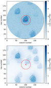 |
Fig. 1 Top panel: field of view of WASP-103 as observed by CHEOPS transit #10. Bottom panel: field of view of WASP-103 simulated by the DRP based on the Gaia catalogue and excluding WASP-103. The red cross marks the target position, while the red circle shows the DEFAULT aperture. The image scale is 1 arcsec per pixel. |
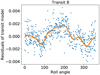 |
Fig. 2 Residuals of the transit fit as a function of the roll angle of the satellite for transit number 8. A clear dependence is seen which is well fitted with a non-parametric GP model overplotted in orange (see Sect. 2.3.1). The best fit length scale hyper-parameter in this case was
|

2.3.1 Multi-dimentional GP
We performed GP regression with a Matern-3∕2 kernel to model the flux dependence on the instrumental parameters using the George package (Ambikasaran et al. 2015). This is coupled with a transit model using a parametrisation and method similar to the one used in Barros et al. (2020). The transit model is parameterised by the orbital period (P), mid-transit time (T0), normalised separation of the planet (a∕R⋆), the planet-to-star radius ratio (rp∕R⋆), inclination (inc), and quadratic limb darkening law. We assumed a circular orbit (Gillon et al. 2014; Delrez et al. 2018 and Sect. 3.1.2). The hyper-parameters of the GP are an amplitude (amp) and a length scale (s).
For the shape parameters of the transit (a∕R⋆, rp ∕R⋆, and inc), we used Gaussian priors based on the results of Delrez et al. (2018). For the limb darkening parameters, we also used Gaussian priors whose values and the uncertainties were derived with the LDTK code (Parviainen & Aigrain 2015; Husser et al. 2013) in the CHEOPS bandpass. For the mid-transit time, we used a uniform prior and we assumed the ephemerides derived by Patra et al. (2020) (T0 = 2456836.29630(07) and P = 0.925545352(94)). For the hyper-parameter length scale, we used a uniform prior based on the range of the instrumental parameter variations. For each instrumental parameter, we computed the maximum range of variations and set this as the maximum possible value of the prior and the minimum was set to be one-sixth of this value to avoid over-fitting. For example, in the case of the roll angle, the prior is uniform between 60° and 360°. We also included a jitter parameter for each light curve. The derived values for the jitter indicate that the errors provided by the DRP pipeline are slightly underestimated by a factor of approximately 1.2.
For each transit, we started by using a 2D GP with the roll angle as the detrending instrumental parameter, then we analysed thecorrelations of the residuals with the other instrumental parameters and added the instrumental parameter with the highest correlations to a 3D GP. We performed model comparison to decide if the instrumental parameter should be added or not. Instrumental parameters were added if the difference of BIC was higher than 3, indicating positive evidence in favour of the more complex model. The procedure was repeated until the residuals showed correlations with the instrumental parameters less than 5% or they were already tested with model comparison. The first three light curves were highly correlated with the background and hence we tested a 2D GP with only the background as a detrending instrumental parameter. This was found to be better only for light curve number 3. This procedure was applied to both the OPTIMAL and the DEFAULT apertures and we chose the one with smaller final residuals. The instrumental parameters chosen with this procedure for the decorrelation of each of the transit light curves as well as the aperture chosen are given in Table 1.
For parameter inference, we used the affine-invariant Markov-chain Monte-Carlo ensemble sampler implemented in emcee (Goodman & Weare 2010; Foreman-Mackey et al. 2013). The fitting procedure was performed in two steps. First we performed a global fit using previously normalised light curves (first order polynomial based on out-of-transit data) and assuming a linear ephemerides and the best detrending GP model. From the global fit, we derived the transit parameters and their uncertainties similarly to Barros et al. (2020). These are given in Table 2 together with the priors used. In the second step, the posterior of the shape parameters a∕R⋆, rp ∕R⋆ and inc derived from the first step were used as priors for a second individual fit to each light curve to derive accurate transit times. In this second step, we simultaneously accounted for a linear normalisation of the transit parameterised by an out-of-transit level (Fout) and flux gradient (Fgrad). Fitting the transit normalisation is important to avoid biases in the derived mid-transit times as shown in Barros et al. (2013). For each light curve, we used the best model GP determined in the previous step with the same hyper-parameters’ priors mentioned above. The two step approach was adopted because the correlations are different for each light curve and the detrending instrumental parameters considered are also different. Therefore, a simultaneous fit of the detrending instrumental parameters would imply a prohibitive number of parameters to fit (317). We performed tests that showed that this approach does not affect the results.
The WASP-103b transit light curves together with the best multi-dimensional GP and transit model, chosen by model comparison, are shown in Fig. 3. The light curves show instrumental effects that are well corrected by the GP model, as can be seen from the well behaved residuals.
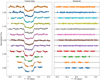 |
Fig. 3 Left panel: transit light curves of WASP-103b obtained with CHEOPS. We overplot our best fit model that includes a transit model and the GP model to account for systematics dependent on the instrumental parameters. Right panel: residuals of the fit of the transit model and the GP model. For clarity, the errors are only shown in the residuals. The light curves and residuals are offset vertically for clarity. |
Priors for the fitted transit parameters.
2.3.2 Pycheops
For comparison, we also analysed the OPTIMAL extracted light curves with pycheops (Maxted et al. 2021), a custom python package developed specially for CHEOPS data. First we used the single visit analysis to determine the best parameters to use as decorrelation instrumental parameters. pycheops performs linear decorrelation with several instrumental parameters such as contamination, background, position of the target on the CCD, and trigonometric functions of the roll angle and its harmonics. As in the multi-GP method, we used priors based on the transit parameters derived in Delrez et al. (2018).
After analysing the data with the single visit model, we used the multivisit mode of pycheops to simultaneously fit the 12 transits and determine the individual transit times. To avoid the large number of fitted parameters, pycheops has implemented a technique (Luger et al. 2017) to perform an implicit decorrelation of several light curves using a GP. A detailed description of pycheops and example applications to CHEOPS data are given in Maxted et al. (2021). The derived transit times with pycheops are closer than 1 σ to the ones derived with the multi-dimensional GP. The derived uncertainties in the transit times are also similar.
3 Complementary observations
3.1 Constraining the companion of WASP-103
Using the lucky imaging technique, a possible companion to WASP-103 was detected at 0.242± 0.016 arcsec by Wöllert & Brandner (2015) on 07 March 2015. They measured the position angle to be 132.7± 2.7 degrees and contrast magnitudes to be Δi = 3.11 ± 0.46 and Δz = 2.59 ± 0.35. These observationswere made with the AstraLux instrument (Hormuth et al. 2008). This companion was later confirmed by adaptive optics (AO) observations using the NIRC2 instrument at Keck (Ngo et al. 2016) on the 25 January 2016. They clearly detect a companion at 0.239± 0.002 arcsec. Within the errors, no change of position was detected between the two observations. These observations were used by Cartier et al. (2017) to perform a spectral energy distribution (SED) fit to the companion and estimate its parameters. This assumes that the companion is located at the same distance as WASP-103 which has not been confirmed. The stellar parameters derived by Cartier et al. (2017) together with the position measurements derived by Ngo et al. (2016) are reproduced in Table 3. According to the AO measurements, if the companion is at the same distance as WASP-103A (552 ± 33 parsec – Gaia EDR3 (Gaia Collaboration 2021) – Table 4), it would be at 131.9± 8 au from WASP-103. If the orbit is circular, thiswould imply a period of 1114 ± 103 yr and a radial velocity (RV) signature with an amplitude of ~ 1334 m s−1.
There is an excess of astrometric noise in the Gaia data that is consistent with the existence of a companion for this system. This noise was present in the DR2 data release and in the recent EDR3. Furthermore, the Gaia derived parallax changed from 1.14± 0.17 in DR2 to 1.82± 0.11 in EDR3 which is a 3.4 σ change, which could be due to a deviation from single-source behaviour induced by a companion. Therefore, the companion still seems to be close to WASP-103 at the present epoch.
Parameters for the companion of WASP-103A.
3.1.1 Lucky imaging observations
To better constrain the companion of WASP-103 and confirm that it is bound, we performed new lucky imaging observations of WASP-103. We used the same instrument that discovered the companion (Wöllert & Brandner 2015), the AstraLux camera (Hormuth et al. 2008) mounted on the 2.2-m telescope at Calar Alto observatory in Almería, Spain. The observations were performed under excellent conditions (seeing 0.7 arcsec) in two filters SDSSi and SDSSz. We obtained 90 000 frames, each with an exposure time of 10 ms.
As shown in Figs. A.1 and A.2, we did not recover the companion found by Wöllert & Brandner (2015) and subsequently characterised Ngo et al. (2016) and Cartier et al. (2017). We computed the sensitivity limits for our images by using the approach described in Lillo-Box et al. (2012, 2014). According to our contrast curve, we should have detected the companion if it was in the same location (separations and position angle). No difference in the position of the companion was detected between the two previous observations (Wöllert & Brandner 2015; Ngo et al. 2016), but they were only separated by 10 months. Assuming that the target observed by us and the previous publications is the same, in order to explain the non-detection of the companion in our AstraLux images, the companion should have moved towards WASP-103A by at least ~ 0.14 arcsecs, which corresponds to ~77 au at the distance to WASP-103 (Table 4).
This is difficult to explain in a scenario where the companion is bound to WASP-103 since the time difference between the observationsis just 6 yr. The maximum velocity of a bound object is lower than the velocity at the periapsis given by the following:
 (2)
(2)
(Murray & Dermott 1999), where G is the gravitational constant and d is the distance of the periapsis. Assuming the periapsis is equal to 131.9 au (Table 3), in 6 yr, the upper limit on the distance travelled by a bound object is 6.4 ± 0.2 au. Therefore, we conclude that either the star is not bound (and hence we are seeing the relative proper motion of both stars, with the background star disappearing behind WASP-103) or much less likely, unknown systematics have prevented its detection in the new observations. Further high resolution images of WASP-103 or the Gaia DR3 will shed light on this system.
Stellar parameters of WASP-103A.
3.1.2 CORALIE RV observations
If WASP-103A has a bound stellar companion, we expect a long-term variation in the observed RVs. Previous RV observations of WASP-103 from the discovery paper and a follow-up paper (Gillon et al. 2014; Delrez et al. 2018) do not show any long-term variation, but they only span 450 days. To constrain the longer-period RV variations, we obtained new RVs of WASP-103 with CORALIE, the same instrument that was used in previous studies. Ten new observations were made between 18 March 2021 and 30 May 2021 which increased the time span of the observations to 8 yr.
The CORALIE spectrograph is installed at the Nasmyth focus of the Swiss Euler 1.2 m telescope (Queloz et al. 2000) and has a spectral resolution of 60 000. The light can be injected through two fibres allowing it to observe the science target and to perform a simultaneous monitoring of the sky or a wavelength calibration with a Fabry Perot etalon. In November 2014, the spectrograph benefited from a major upgrade, which introduced an RV offset which we modelled as a simple offset between the two sets of data. The observations were processed with the standard data reduction pipeline. The RVs were derived with the weighted cross-correlation technique (Pepe et al. 2002) and a G2 mask was used as it is optimised for late F-type stars such as WASP-103.
The RVs were analysed with the code LISA (Demangeon et al. 2018, 2021) which uses the radvel python package (Fulton et al. 2018) to model the RV observations. The RV model is parameterised by the semi-amplitude of the RV signal (K), the planetary period (P), the mid-transit time (T0), and the products of the planetary eccentricity by the cosine and sine of the stellar argument of periastron e cosω, e sin ω. We used Gaussian priors for the planetary orbital period and mid-transit time based on the constant period model derived in Sect. 4. We included an offset between the new RV observations and the previously published RV observations to account for the RV shift due to the upgrade of the instrument mentioned above. We also included a jitter parameter for each dataset to account for unknown systematic noise or short-term stellar activity. We compared a model with a beta prior on the orbital eccentricity (Kipping 2013b) with a circular model. Due to the short time span of the observations compared with the expected orbital period of the possible binary, the visual companion, if bound, would lead to a trend in the RV observations. Moreover, given the short span of the two epochs of observations and the large gap between them, this trend can be represented by an offset between both observations. Therefore, the fitted offset is a combination of the instrumental offset and the trend due to the possible companion star.
With the free eccentricity model, we found a non-significant eccentricity of 0.11 ± 0.06. The difference between the Bayesian information criterion (BIC) of the eccentric and circular model is 0.011 which implies thatthe eccentric model is not justified. As mentioned above, due to the very short orbital period of WASP-103b, the orbit of the planet is expected to be circularised and the rotation of the planet synchronised with the orbital period. Therefore, we adopted the circular model for the planet. We found a semi-amplitude K = 268 ± 14 m s−1 in agreement with previous results (Delrez et al. 2018). We also found an offset between the previous observations and the new observations of 14 ± 45 m s−1. At 3 σ, we can exclude an offset higher than 151 m s−1 and lower than − 119 m s−1. The relativeoffset due to the instrumental upgrade between the two observations is expected to be between 14 and 24 m s−1 (CORALIE team priv. comm.). Therefore, we conclude that there is no significant offset between the new and the previous observations of WASP-103b. At 3 σ we can also exclude RV variations higher than 151 − 24 = 127 m s−1 and lower than − 119 − 24 = −143 m s−1 over 8 yr. Asoutlined in Sect. 4.1, this limit on the amplitude of the RV variation does not allow us to discard the bound scenario.
3.2 Stellar parameters
Thanks to the new data release of Gaia, the stellar parameters of WASP-103A can be better constrained, which in turn allowed us to better constrain the mass and radius of the exoplanet WASP-103b. Using a modified version of the infrared flux method (IRFM; Blackwell & Shallis 1977), we determined the radius of WASP-103A via relationships between various stellar parameters recently detailed in Schanche et al. (2020). We constructed the SED from stellar atmospheric models using the stellar parameters from SWEET-Cat (Sousa et al. 2018) as priors, and subsequently attenuated the SED to account for reddening. The SED was further corrected for the companion using the calculated contamination estimate from the stellar parameters for the companion in Cartier et al. (2017) and reproduced in Table 3. The corrected SED was then convolved with broadband response functions for the chosen bandpasses to obtain synthetic photometry which allowed us to compute the bolometric flux, and hence the radius, of the target. We retrieved broadband fluxes and uncertainties from the most recent data releases for the following bandpasses: Gaia G, GBP, and GRP; 2MASS J, H, and K; and WISE W1 and W2 (Skrutskie et al. 2006; Wright et al. 2010; Gaia Collaboration 2021). We also used the ATLAS catalogues (Castelli & Kurucz 2003) of model stellar SEDs. Within the IRFM, the distance used to convert the angular diameter of WASP-103A to the stellar radius was calculated from the Gaia EDR3 parallax with the parallax offset of Lindegren et al. (2021) being applied. Using a Markov chain Monte Carlo (MCMC) fitting approach, we estimated the stellar radius of WASP-103A to be R⋆ = 1.716 ± 0.119 R⊙. This is larger than the previous estimates, that is 1.436 ± 0.052 (Gillon et al. 2014) due to the greater distance to WASP-103 derived from the EDR3 parallax.
We derived both the stellar mass M⋆ and age t⋆ by employing two different sets of stellar evolutionary models, namely PARSEC v1.2S1 (Marigo et al. 2017) and CLES (Code Liégeois d’Évolution Stellaire Scuflaire et al. 2008). The input parameters we used were the stellar [Fe/H], Teff, and R⋆ to locate the star on the Hertzsprung–Russel Diagram (HRD) plus the projected rotational velocity v sini, which was plugged into the gyrochronological relation by Barnes (2010) to remove isochronal degeneracies; for further details, see Bonfanti & Gillon (2020, Sect. 2.2.3). We performed a direct interpolation of the input parameters within pre-computed grids of PARSEC models thanks to the isochrone placement algorithm presented in Bonfanti et al. (2015, 2016), obtaining the first pair of age and mass values. The second pair was inferred by directly computing the evolutionary track through the CLES code and then choosing the best-fit solution following the Levenberg-Marquadt minimisation scheme (Salmon et al. 2021). After checking the consistency of the two mass and age values following the χ2 criterion discussed in detail in Bonfanti et al. (2021), we combined the respective distributions of age and mass together to obtain our final estimates of M⋆ and t⋆. The mass is in agreement with previous estimates, while the age is much better constrained (Gillon et al. 2014; Delrez et al. 2018). The final stellar parameters and the 1 σ uncertainties are given in Table 4.
3.3 Re-analysis of previous transits
Given the very high signal-to-noise required to detect the tidal deformation, we have re-analysed high signal-to-noise transits of WASP-103 previously obtained with the Spitzer and Hubble space telescopes. These are combined with the 12 new transits obtained with CHEOPS in our final analysis.
3.3.1 Spitzer observations
We re-analysed the Spitzer archival data of WASP-103b which has already been published (Kreidberg et al. 2018). We downloaded WASP-103b archival IRAC data from the Spitzer Heritage Archive2. The data consist of one full phase curve of WASP-103b at 4.5 μm (channel 2) and one at 3.6 μm (channel 1), both were obtained under program ID 11099 (PI L. Kreidberg) taken on 19 and 28 May 2015. The reduction and analysis of these datasets are similar to Demory et al. (2016a). We modelled the IRAC intra-pixel sensitivity (Ingalls et al. 2016) using a modified implementation of the BiLinearly-Interpolated Sub-pixel Sensitivity (BLISS) mapping algorithm (Stevenson et al. 2012). We used a modified version of the BLISS mapping (BM) approach to mitigate the correlated noise associated with intra-pixel sensitivity. In our photometric baseline model, we complement the BM correction with a linear function of the point response function (PRF) full width at half-maximum (FWHM).
In addition to the BLISS mapping, our baseline model includes the PRF’s FWHM along the x and y axes, which significantly reduces the level of correlated noise as shown in previous studies (e.g. Lanotte et al. 2014; Demory et al. 2016a,b; Gillon et al. 2017; Mendonça et al. 2018). Our baseline model does not include time-dependent parameters. Our implementation of this baseline model is included in an MCMC framework already presented in the literature (Gillon et al. 2012). We ran two chains of 200,000 steps each to determine the phase-curve properties and obtained the best detrended transit light curves which are analysed together with HST and CHEOPS transits in Sect. 5. From our BM+FWHM baseline model, we obtained a median root mean square (RMS) of 3450 ppm per 10.4 s integration time at 3.6 μm and 4480 ppm with the same integration time at 4.5 μm.
3.3.2 HST observations
We re-reduced the Hubble transit observations taken on 26–27 February 2015 and 2 August 2015 with HST Program 14050 which were originally published by Kreidberg et al. (2018). The target was acquired in both forward and backward scanning direction using an exposure time of 103 s. We used the frames in the IMA format, each one containing 16 non-destructive reads (NDR; Deming et al. 2013), which were pre-processed by the CALWFC3 pipeline3, version 3.5.2.
Wavelength calibration, NDR operations, background subtraction, cosmic ray and bad pixels rejection, and correction for drifts were carried out following standard procedures, as described in Bruno et al. (2018, and references therein). Then, we integrated the stellar spectra in the 1.115–1.625 μm wavelength range to obtain the band-integrated transits. Following standard practice (e.g. Deming et al. 2013), we rejected the first HST orbit of the transit obtained on 2 August 2015, which was at the beginning of the phase curve observation, and the first data point of every orbit for both transits.
We then used a method similar to Kreidberg et al. (2018) to remove the instrument systematics with the model described in Stevenson et al. (2014), that is with a second-order polynomial and an exponential ramp,
 (3)
(3)
where we fitted for C and r0−4, and θ and ϕ represent the planetary and HST phase, respectively. It was also necessary to add a shift to the HST orbital phase, ϕ =2π[(t − ψ) mod PHST]∕PHST, where ψ =−0.045 d is for the February 2015 visit and ψ = −0.1 days is for the August 2015 visit, respectively, and PHST is Hubble’s orbital period.
The systematics were fitted simultaneously with the transit model of a non-deformed planet using the model of Mandel & Agol (2002)(implemented in Kreidberg (2015) software) and scipy’s optimize.minimize function (Virtanen et al. 2020, and references therein). The best detrended transit light curves are analysed together with Spitzer and CHEOPS transits in Sect. 5. The mid-times of each exposure were converted to BJD-TDB using the online applet based on the method of Eastman et al. (2010).
Derived mid-transit times of WASP-103b.
4 Period evolution of WASP-103b
Using the procedure outlined in Sect. 2.3.1, we obtained the mid-transit times of the CHEOPS observations. These are given in Table 5. In this table, we also included the mid-transit times derived for the Spitzer and HST transits. We reiterate that the derived CHEOPS transit times obtained with our method are within 1 σ of the ones derived using pycheops showing that our detrending methods are robust.
We combined our derived mid-transit times (12 + 4) with the 32 previously published mid-transit times of WASP-103 which were presented in Table 3 of Maciejewski et al. (2018), some of which are reanalyses of previously published values (Gillon et al. 2014; Southworth et al. 2015; Delrez et al. 2018; Turner et al. 2017; Lendl et al. 2017). We also added the four transit times subsequently presented in Patra et al. (2020). Therefore, in total we have 52 mid-transit times of WASP-103b spanning 7 yr.
For parameter inference, we used emcee as in Sect. 2.3.1. We compared a linear ephemerides (constant period) model with a quadratic ephemerides (constant derivative period) model. We included a multiplicative jitter parameter in our analysis.
For the constant period model, we obtained  and P = 0.925545485 ± 0.000000049 days. The BIC of this fit is 79.8. We found a jitter of 1.18.
We considered a constant derivative period model with the following form (e.g. Maciejewski et al. 2020):
 (4)
(4)
where E is the transit epoch and Ṗ is the period derivative.
For this model we derived T0 = 2457511.944344 ± 0.000075(BJDTDB), P = 0.9255453 ± 0.000000089 days, Ṗ = 3.5 ± 1.8 × 10⁻¹⁰ days day−1, and jitter = 1.15. The jitter is slightly lower than for the linear model. We found a hint of an increasing orbital period, contrary to what was expected if tidal decay was dominating the orbital evolution of the system. The period derivative was found to be positive at 2.1 σ which is not significant. The BIC of the quadratic model is 78.05, giving a difference of BIC in favour of the quadratic model of only 1.8. Therefore, according to the BIC, the added complexity of the quadratic model is not strongly justified and the linear ephemerides is preferred.
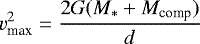
Under assumption that the period variation observed is due to tidal decay (i.e. the period is actually decreasing and the variation seen is due to statistical uncertainties), we can derive a lower limit to the tidal dissipation parameter using the following equation (e.g. Maciejewski et al. 2020):
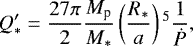 (5)
(5)
where Mp and M* are the planetary and stellar masses, respectively, R* is the stellarradius, and a is the semi-major axis of the planet’s orbit. We derived a lower limit on the period derivative to be − 1.3 × 10⁻¹⁰ days day−1 at the 99.7% confidence interval. This implies that the tidal dissipation parameter is higher than 1.6 × 10⁶ at 3 σ, corresponding to a 99.7% confidence interval if we assume that only tidal decay affects the period derivative. This limit is more than an order of magnitude higher than previous studies that found  at 95% (Patra et al. 2020) for WASP-103b. At 95% confidence, our results allow us to exclude a negative period derivative. The quadratic fitto the derived transit times is given in Fig. 4. We found a period derivative that is smaller than the previous estimation (Patra et al. 2020), although the higher precision results in a higher significance for being positive.
Figure 4 shows that the first two CHEOPS transits have a slightly late mid-transit time compared with the other observed CHEOPS transit times, although consistent within the errors. This is probably due to the difficulty in detrending CHEOPS data when the duration of the visit is shorter than three CHEOPS orbits. It is also known that transits with poorly covered ingress or egress can lead to biases in the derived transit times (Barros et al. 2013). To test if this could influence our results we repeated the linear and quadratic model fits excluding the first two transits. We found no significant differences in the derived model parameters or model comparison. We also repeated the fits using the transit times derived with pycheops instead of the ones derived with the multi-dimensional GP and found the same results.
Although it is likely that the observed period variation is due to statistical dispersion and that the orbit is decaying due to tides, it is interesting to explore other factors that could affect the orbital evolution of this system. In the next subsections, we explore scenarios that could explain an increase in the orbital period in case it becomes significant after future observations.
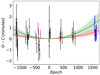 |
Fig. 4 Derived mid-transit times of WASP-103b after removing a linear ephemerides. The CHEOPS data are shown in blue, the re-reduced HST data and Spitzer are shown in magenta, and the previously published times are shown in black. The previously published quadratic ephemerides (Patra et al. 2020) is shown in green with the 1 σ uncertainty limit, while our new result is shown in red. |
4.1 RV acceleration due to a companion
The existence of a companion of WASP-103 could lead to RV acceleration which would produce transit timing variations due to a change in the light travel time. Assuming a quadratic ephemerides and that the observed period derivative is due to the Doppler effect of a line-of-sight acceleration (ṖRV), we can derive the line-of-sight acceleration (ar) using the following:
 (6)
(6)
where c is the speed of light. We obtained ar = 0.113 ± 0.058 m s−1 day−1.
During the 8 yr since the discovery of WASP-103b until now, this would imply an RV variation of 330 ± 168 m s−1. This is higher than the RV offset that we measured in Sect. 3.1.2, but it is still compatible within the errors.
We can also calculate the expected acceleration from the visual companion of WASP-103 if it is bound (discussed in Sect. 3.1) using Newton’s law:
 (7)
(7)
where Mcomp is the mass of the visual companion star and d is the separation between the two stars. In this case, where the companion is observed to be spatially separated from WASP-103, we need to account for the projection of the acceleration in the line-of-sight given that only the radial component of the acceleration results in a variation of the observed period. If the angle between the line-of-sight and the companion is θ, then arad = acosθ and d = δ∕sinθ. Where δ is the projected separation of the star and the companion that we previously derived (Sect. 3.1) as 134 ± 8 au. Hence,
 (8)
(8)
The maximum value of Eq. (8) is obtained for  . Assuming Mcomp = 0.721 ± 0.024 M⊙ (Table 3), we can set an upper limit on arad ≤ 0.00796 ± 0.00095 m s−1 day−1. This corresponds to an RV acceleration of 23.6± 2.7 m s−1 in 8 yr. Thisis compatible with the RV offset that we measured between the new CORALIE observations and the previously published observations (Sect. 3.1.2). The difference between the acceleration expected if the transit timing variations are due to acceleration from a bound companion and the acceleration from the observed visual companion is 0.105 ± 0.057 m s−1 day−1. Hence, the acceleration produced by the visual companion is probably not enough to produce the period derivative estimated with the quadratic model. However, we cannot exclude it at more than 2 σ.
Long-term RV monitoring of WASP-103b and the next Gaia DR3 will allow us to better constrain the existence of possible bound companions to WASP-103 and correct the line-of-sight acceleration light travel time, allowing us to better constrain the tidal dissipation parameter. The hypothesis that the visual companion observed by lucky imaging and AO observation is responsible for the transit timing variations and the offset in CORALIE RVs cannot be completely rejected. However, the absence of this star in our new lucky imaging observation and the fact that the predicted acceleration by this star is 2 σ lower than required to match the observations, suggests that other mechanisms would be required to explain an increase in the orbital period of the planet.
4.2 Applegate effect
Eclipse times of binary stars have been shown to vary due to variations in the quadrupole moment of the stars driven by stellar activity. Low mass stars with convective outer layers have variations of their quadrupole moment due to a distribution of angular momentum driven by stellar activity cycles. The change of the quadrupole moment of the star leads to quasi-periodic variations of the eclipse times of the companion over timescales of years to decades. This effect has been measured in many eclipsing binaries and is known as the Applegate effect (Applegate 1992). Another explanation for the observed period changes in binaries was proposed by Lanza et al. (1998). In this case, the Applegate effect would be due to a cyclic transformation of rotational kinetic energy into magnetic energy and back to rotational kinetic energy. If the Applegate effect is detected, it would allow us to probe the nature of the dynamo mechanism of low mass stars (Lanza et al. 1998).
Since exoplanets host low mass stars with some dynamo activity, it is expected that the Applegate effect is also present in exoplanet systems; although, it has never been observed. Watson & Marsh (2010) estimated the transit time variations due to the Applegate effect for a few transiting exoplanets. They show that for stellar dynamos with timescales of 11 yr, the Applegate effect is less than 5 s for most exoplanet host stars. However, for stellar dynamos with longer timescales, the effect can reach a few minutes. Using their equation 13 and assuming the stellar parameters given in Table 4, the semi-major axis of the orbit a = 0.01985 au, the observation time span T = 7 yr, and estimating the stellar angular rotation velocity of WASP-103 from the v sin i given in Gillon et al. (2014) (10.6 km s−1), we concludethat the Applegate effect in WASP-103b would produce transit timing variations ≤ 38 seconds over the time span of the available observations. Assuming the quadratic ephemerides, we found that at the mid-epoch of CHEOPS observations, the measured transit time, is 1.69± 0.81 minutes later than what would be expected by a linear ephemerides. Therefore, this is higher than the expected timing variations from the Applegate effect, although in agreement at 1.3 σ. Hence, we conclude that the Applegate effect could be affecting the measured transit times of WASP-103b.
4.3 Apsidal precession
If a planet’s orbit is slightly eccentric, then its orbit would be apsidally precessing. For hot Jupiters, the precession timescale is expected to be decades. In this case, there is a long-term oscillation of the apparent period. Modelling the period variation would allow us to determine the planet Love number and constrain its internal structure. For WASP-103b, a zero eccentricity was assumed by Gillon et al. (2014) and favoured by the analysis of Delrez et al. (2018) and our own analysis using the new RV measurements presented in Sect. 3.1.2.
Nevertheless we attempted to fit the times of WASP-103 with a transit timing model assuming apsidal precession (Patra et al. 2017):
 (9)
(9)
where,
 (10)
(10)
We found that the apsidal precession model is a poor fit to the transit times with a BIC = 82.7. This is due to the two extra parameters compared with the quadratic model that is already not justified by the BIC compared with the linear model. However, we obtained physical values for the fitted parameters. We obtained 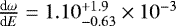 rad,
rad, 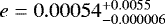 , and
, and 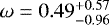 rad.
rad.
The most important contributions to the apsidal precession rate of hot Jupiters are those coming from the tides raised by the star on the planet and from the rotation of the planet (Ragozzine & Wolf 2009). Assuming synchronous rotation, the leading term in the expression of this precession rate at low eccentricity is as follows (see, e.g. Eqs. (6) + (10) of Ragozzine & Wolf 2009):
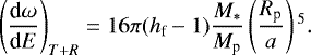 (11)
(11)
Using our fitted value for the precession rate of  rad, we can estimate the Love number to be hf = 1.35 ± 0.43, which is compatible with our estimate from the deformation of the light curve (Sect. 5).
Current observational constraints on the eccentricity cannot rule out such a small value ~ 0.00054. However, due to the short circularisation timescale, the eccentricity of WASP-103b is expected to be zero unless there is an external perturbation. For example, a planetary companion can excite the eccentricity of WASP-103b. The eccentricity can also be excited by gravitational perturbations from the star’s convective eddies as proposed by Phinney (1992).
Therefore, we cannot completely rule out that apsidal precession is affecting the transit times of WASP-103b given our current constraints on the eccentricity of the planet although this is, a priori, not expected. Future monitoring of the transit times of WASP-103b can disentangle apsidal precession from tidal decay since for apsidal precession the variations are sinusoidal. The times of occultation can also be used to disentangle both scenarios because in the apsidal precesion, these are anti-correlated with the times of transit.
5 Tidal deformation analysis
As mentioned above, WASP-103b is the exoplanet with the highest expected deformation signature due to its large radius and close proximity to its host star. We attempted to measure the deformation and tidal Love number of WASP-103b, combining the 12 new high-precision transits obtained with CHEOPS with two HST transits and two Spitzer transits (3.4 and 4.5 μm). To model the tidal deformation, we used the implementation of Akinsanmi et al. (2019) based on the parametrisation of Correia (2014). This implementation uses the ellc transit tool (Maxted 2016) and it is also freely available. The model parameters are the normalised separation of the planet (a∕R⋆), the impact parameter (b), the Love number (hf), the logarithm of the planet-to-star mass ratio multiplied by the sine of the inclination ( ), and, for each filter, the planet-to-star radius ratio (RV∕R⋆) and the power-2 limb darkening (LD) coefficients (c and α). Following Eq. (1), in this ellipsoidal model, the radius of the planet is parameterised by the volumetric radius
 ![Mathematical equation: $R_{V} =\sqrt[3]{r_1r_2r_3}$](/articles/aa/full_html/2022/01/aa42196-21/aa42196-21-eq32.png) . The LD coefficients were parameterised according to Kipping (2013a) and Short et al. (2019) to minimise the correlations between them and to avoid non-physical solutions.
. The LD coefficients were parameterised according to Kipping (2013a) and Short et al. (2019) to minimise the correlations between them and to avoid non-physical solutions.
The priors for each parameter are given in Table 6. For the shape parameters, we used uniform uninformative priors instead of normal distributions based on previous data because the previous results were obtained assuming sphericity, which impacts the derived shape parameters. We assumed the period and mid-transit times derived in Sect. 4. We included a multiplicative jitter term for CHEOPS, HST, and Spitzer channel 1 and channel 2 to account for any underestimation of the uncertainties. For each light curve, we corrected the contamination due to the visual companion star (see Sect. 3.1), assuming the stellar parameters given in Table 3 and the respective filter transmission functions.
For the parameter inference, we used the nested sampling algorithm implemented in Dynesty (Speagle 2020; Higson et al. 2019; Skilling 2012, 2004) which provides posterior estimates and also the Bayesian evidence useful for model comparison. We fitted the tidal deformation parameterised by hf and compared it with a spherical model (hf = 0). The comparison of the models illustrates biases in the derived shape parameters if the deformation is ignored. The derived transit parameters are given in Table 7 for the spherical and the ellipsoidal model. The derived jitter parameters for the ellipsoidal model are 1.00, 1.11, 1.21, and 1.09 for Spitzer channel 2, Spitzer channel 1, CHEOPS, and HST, respectively, showing that our errors are robust and the detrending was successful. The derived jitter parameters for the spherical model are similar to the ellipsoidal model.
We overplotted the best model that accounts for tidal deformation on the time-folded light curves of WASP-103b taken with Spitzer 2, Spitzer 1, CHEOPS, and HST in Fig. 5. We also show the residuals of the spherical model and overplotted the difference between the best fit spherical model and the best fit ellipsoidal model. As shown by Akinsanmi et al. (2019), this is the measurable signature of the deformation of a planet in a transit light curve. This signature has two components. The first one is the signature of the oblateness (r2 > r3) resulting in an oscillation in the residuals of the flux during ingress and egress (Seager & Hui 2002; Barnes & Fortney 2003). The second one rises from r1 > r2 due to the change of the projected area of the ellipsoidal planet as it rotates synchronously with its orbit. This results in a bump that has its maximum at the minimum of the projection which is the middle of the transit (Correia 2014). A schematic view of the geometry of how the deformation changes a transit light curve is given in Fig. A.1 of Correia (2014). The change in the amplitude of signature of the deformation with the wavelength of the observations due to the change in the limb darkening and the larger planetary radius at longer wavelengths, as it can be seen in Fig. 5, is noteworthy. This prevented us from phase folding all light curves and signatures so that our results could be visualised better.
In Fig. 6, we show the correlation plots and the posterior probability distributions for the derived transit parameters of WASP-103b. As expected, there is a large correlation between the Love number and the radius ratio for the ellipsoidal model that leads to a larger uncertainty of the parameters of this model. For simplicity, we do not show the distribution of the LD parameters and the jitter parameters because their shape is very well approximated by a Gaussian and they are very similar for the two models.
We derived the radial Love number of WASP-103b to be  . This is the first time that a 3 σ detection of the Love number has been achieved for an exoplanet directly from the analysis of the deformation of the transit light curve. To obtain this result we combined the datasets from the three instruments: CHEOPS, HST, and Spitzer. To show the importance of each data set, we fitted the Spitzer and HST light curves separately and together. These results are given in Table 8 and show that the addition of the CHEOPS data was necessary to obtain a 3 σ detection. Italso justifies that the signature is not evident by eye in Fig. 5 for any individual datasets. We conclude that the Love number of WASP-103b is similar to the Love number measured for Jupiter (1.565 ± 0.006 – Durante et al. 2020), suggesting a similar internal structure despite the much larger radius and much higher levels of irradiation for this exoplanet. The derived Love number of WASP-103b is higher than the one estimated for HAT-P-13b by Batygin et al. (2009). This new measurement of the Love number can be used to lift the degeneracy of internal composition models (Baumeister et al. 2020) and allows the derivation of the core mass of WASP-103b similarly to what was done for HAT-P-13b (Kramm et al. 2012; Buhler et al. 2016).
We found that the volumetric radius derived with the ellipsoidal model is 5–6% bigger than the radius estimated with the spherical model. Therefore, not accounting for deformation biases the derived planetary radius and hence the planetary density (~ 14%) and composition. This is the first time that this bias that was predicted by Burton et al. (2014) and Correia (2014) has been directly measured. The large tidal deformation in ultra-hot Jupiters affects their phase curve observations and consequently their atmospheric characterisation. Previous phase curve measurements of WASP-103b (Delrez et al. 2018; Lendl et al. 2017; Kreidberg et al. 2018) have corrected tidal deformation using theoretical estimations (e.g. Budaj 2011; Leconte et al. 2011) that assume an interior structure for the planet. Our measurement of the Love number will allow an assumption-free correction based on direct observations. This will allow a more accurate estimation of the day-side and night-side temperatures from phase curve observations. It is also possible that neglecting to account for the deformation of WASP-103b could affect the interpretation of its transmission spectra (Lendl et al. 2017).
Priors for the fitted transit parameters.
Derived transit parameters of WASP-103b for an ellipsoidal planet model and a spherical model.
Comparison of the derived Love number for the individual instruments and their combination.
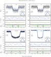 |
Fig. 5 Time folded transit light curves of WASP-103b obtained with Spitzer 1, Spitzer 2, CHEOPS, and HST. The CHEOPS transit light curve is a combination of 12 individual transits, while the HST light curve is a combination of two transits. The best fit ellipsoidal transit model is shown in blue. We also plotted the residuals of the best fit ellipsoidal model (blue) and the best fit spherical model (red) binned to 5 min. On the latter, we overplotted the signature of the deformation(green) which is the difference between the best fit spherical model and the best fit ellipsoidal models. For clarity, we replotted a zoom of the signature of the deformation in the bottom panel for each filter. We also show the mean uncertainties of the original data points and of the binned residuals. |
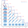 |
Fig. 6 Derived correlation plots and posterior probability distributions of the transit parameters of WASP-103b for the spherical (red) and ellipsoidal model (blue). The vertical lines show the median of the distributions and the shaded area shows the 68% confidence intervals. We show the 1 σ (dark blue and dark red) and 2 σ (light blue and light red) contours. We obtained a 3 σ detection of the Love number. The parameter distributions also clearly show that the ellipsoidal model is not as well constrained as the spherical model due to strong correlations between the Love number and the radius ratio. For the ellipsoidal model, the radius ratio refers to the volumetric radius. The superscripts sp1, sp2, ch, and hst refer to the two Spitzer channels, CHEOPS, and HST, respectively. |
5.1 Assessing the significance of the detection
One way to assess the significance of the detection is to perform model comparison – probability of one hypothesis versus another. Bayesian model comparison requires computing the odds ratio between two hypotheses (e.g. Díaz et al. 2014). The odds ratio is the multiplication between the prior odds and the Bayes factor (ratio of the Bayesian evidences). The prior odds are the a priori probability of each model. Given the strong tidal forces WASP-103b is subjected to by its host star, theoretically, we know that the planet has to be deformed. Hence, the prior probability of the spherical model is zero which implies that the odds ratio in favour of the ellipsoidal model is infinity and renders the Bayes factor irrelevant. Nevertheless, we estimated the Bayes factor of the ellipsoidal compared with the spherical model using the evidence computed with Dynesty. We found the Bayes factor (ratio of the Bayesian evidences) of the ellipsoidal compared with the spherical model to be 9.1, giving positive evidence for the ellipsoidal model (Kass & Raftery 1995). However, the Bayes factor penalises more complex models which is incorrect in our case since, as mentioned above, the planet is expected to be deformed and not accounting for deformation significantly biases the derived transit parameters, especially the planetary radius. To correct the penalisation of the extra parameters, we fitted an ellipsoidal model with a fixed value of hf and ln Qm, corresponding to the best fit model. We found the Bayes factor rises to 17.2. Hence, according to this corrected value for the Bayes factor, the ellipsoidal model is 17 times more probable than the spherical model meaning that the data show positive evidence for the deformation model.
Furthermore, in our case we do not need to compare two hypothesis but we need to access the detectability of a measurement and hence we should use parameter inference instead of model comparison. Hence, instead of answering the question of whether the planet is deformed we answer the question of how much the planet is deformed. This latter question is best assessed by the analysis of the posterior probability distribution of hf which measures the deformation rather than by model comparison. Since we found that the distribution of hf does not include the spherical model (hf = 0) at 3 σ, we conclude that the deformation was detected. Using the posterior distribution of hf, we can compute more accurate limits on the detection given that the distribution is not completely Gaussian. We found that hf is higher than 0.18 at the 99.7 confidence limit (3 σ) and hf is higher than 0.03 at the 99.95 confidence limit (3.5 σ). Hence, the detection is slightly higher than 3 σ.
5.2 Impact of limb darkening
The model of the limb darkening can affect the measurement of the Love number (Akinsanmi et al. 2019; Hellard et al. 2019). Despite several studies on the best way to model the LD in exoplanet light curves (Csizmadia et al. 2013; Howarth 2011), consensus still eludes us as it appears that the best model might depend on the quality of the data being analysed (e.g. Espinoza & Jordán 2015). Of the several LD parametrisations, the non-linear law (Claret 2000) is usually regarded as the best description of the stellar intensity profile (Howarth 2011); however, when fitting the parameters in the transit light curves, the correlations between the four parameters can lead to non-physical models. Recently, the power-2 law (Hestroffer 1997) has been shown to be a good balance between a small number of parameters and being a good approximation of the stellar intensity profiles (Morello et al. 2017). Therefore, it has gained much interest helped by a faster algorithm (Maxted & Gill 2019). The most commonly used LD law is the quadratic law (Kopal 1950) due to its relative simplicity, fast implementation, and the existence of several parametrisations to minimise correlations between thetwo parameters (e.g. Kipping 2013a). In addition to the choice of the parametrisation, it is also unclear if it is best to fix the LD coefficients to theoretical values based on stellar models or directly fit the LD in the light curves. The best approach depends not only on the precision of the light curves (e.g. Espinoza & Jordán 2015), but also on the geometry of the system (e.g. Howarth 2011) and on whether the star is active (Csizmadia et al. 2013).
We assessed if the LD model affected the measurement of the Love number by performing several tests. We compared the results for three different LD laws: the quadratic law which is the most widely used, the non-linear 4-coefficient law considered to be the best model, and the power-2 law which has been shown to give good results despite its simplicity. We fitted the LD coefficients using priors derived from the stellar models. We found that the results depend on the priors. In particular, if the priors were very large, the results are independent from the stellar models. This results in a loss of information and loss of correlations between the four different colours which is not ideal since they relate to the same star. Therefore, to try to have LD coefficients that are consistent for our four instrument filters, we investigated which were the smallest reasonable priors for the parameters for each law. To achieve this, we compared the stellar intensity profiles from the ATLAS9 models (Castelli & Kurucz 2003) with the ones from the PHOENIX models (Husser et al. 2013). We used the LDTK code (Parviainen & Aigrain 2015) to fit the limb darkening laws mentioned above for the four filters increasing the intrinsic uncertainty of the models, which account for the uncertainty in the stellar parameters, in order to obtain modelled law uncertainties that encompass both the PHOENIX and the ATLAS stellar intensity profiles. This required increasing the intrinsic model uncertainties by 5–40× for the quadratic and the power-2 law. The factor is higher for the visual filters than for the infrared. For the non-linear law, there is no need to increase the model uncertainties because the four parameters give sufficient flexibility for the model to encompass both sets of stellar intensity profiles. The uncertainty of the modelled LD law was derived by randomly drawing LD coefficients from a Gaussian distribution centred on the LD value and standard deviation equal to its uncertainty. An example, of the fit for the HST filter is shown in Fig. 7. For CHEOPS, we could not derive the intensity profile for the ATLAS models so we used the KEPLER filter, which is similar to CHEOPS, as a proxy for the uncertainties needed. Moreover, for Spitzer, we needed to redefine the stellar radius for the PHOENIX models in order to match the stellar radius of the ATLAS models since in this case the automatic limb definition does not give optimal results (Parviainen & Aigrain 2015; Espinoza & Jordán 2015).
From Fig. 7, it is clear that the PHOENIX and the ATLAS models predict different stellar intensity profiles close to the stellar limb. It is also clear that the power-2 law matches the ATLAS models better and that the non-linear law matches the PHOENIX models better (the latter is by construction). A comparison between LD derived from transit light curves and from theoretical models by Espinoza & Jordán (2015) suggested that the ATLAS models might be a better match to the transit fitted LD coefficients. However, this conclusion might depend on several factors that have yet to be investigated. Therefore, we expect that the quadratic law will be a poor description of the true stellar intensity profile and that the power-2 law will be a good description if the ATLAS models are closer to the true stellar intensity. We also expect that the non-linear LD law has enough flexibility tomatch both cases.
The uncertainties of the LD coefficients derived with the procedure described above were used to set the priors on LD coefficients for the transit light curve fit for the spherical and the ellipsoidal model. The quadratic LD coefficient priors are given in Table B.1, while the non-linear LD coefficient priors are given in Table B.2. The priors and results for the adopted model – the power-2 law – were already given in Sect. 5. We find that despite its simplicity, the power-2 law gives results in good agreement with the more complex non-linear limb darkening law. For the three LD laws that we tested, we obtained consistent results with all of the fitted parameters agreeing within 1 σ. In Table 9, we give the derived Love number, the significance of the detection, and the Bayes factors. As mentioned above, for model comparison, the Bayes factors should be multiplied by the prior odds that are very strongly in favour of the ellipsoidal model. The significance of the results varies slightly, but it agrees well between the models supporting the robustness of our results. For both the power-2 law and the non-linear law, we obtained a detection of the Love number of WASP-103b at more than 3 σ and consistent with each other. It is noteworthy that although the quadratic law provides results compatible within 1 σ with the other laws, it yields the smallest value and the largest uncertainties for hf. This supports the idea that it is the worst model of the three. Since the three models agree well within 1 σ, we conclude that our treatment of the limb darkening is robust and it is not biasing the results.
If we increase the uncertainties of all the priors of the LD coefficients, for example to 0.1, we still obtain consistent values for hf, despite, as expected, the detection significance being reduced to ~2 σ. However, wethink this overestimates the true uncertainty of the LD, especially in the infrared where the LD signature is much smaller. If we use the intrinsic uncertainties derived from the theoretical stellar grids that are much lower than the ones we derived with our method (up to 40×), we find Love number values that are too high, indicating that the LDs were biasing the retrieval of the Love number. Therefore, we find that the best approach is to use as much prior information from the theoretical stellar grids as possible, while taking the differences associated with different models into account (in our case ATLAS and PHOENIX).
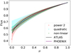 |
Fig. 7 Stellar intensity profiles from the PHOENIX (solid purple line) and ATLAS (solid black line) stellar grids for the HST WFC3.IR.G141 filter as a function of μ
( |
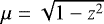
Comparison of the derived Love number, significance of the detection, and Bayes factors for the three LD laws considered.
5.3 Future prospects of measuring the tidal deformation
Since the Love number is an important constraint for interior models, we tested the possibilities of constraining it better. A higher significance of the result would also be desirable for a more robust detection which requires more high signal-to-noise transits of WASP-103b. We simulated more seasons of CHEOPS observations, assuming in each season we would observe 12 more transits. If we could obtain four more seasons of observations (48 transits over 4 yr), we would be able to measure the Love number of WASP-103b at 4.3 σ. If we could obtain six more seasons of observations (72 transits over 6 yr), we would be able to derive hf at 5 σ. This would require the CHEOPS mission being extended.
The extreme high precision of James Webb Space Telescope (JWST) and the fact that the limb darkening signature is lower in the infrared implies that the best chances of significantly increasing the precision of the measurement of the Love number in the near future is to combine our data with a transit with JWST. Since we are interested in maximising the cadence and the signal-to-noise of the observations, the best would be to use the NIRSpec Prism mode which would enable a precision of 62 ppm/min. We simulated a transit of WASP-103b with NIRSpec Prism mode assuming the Love number derived above. We assumed a limb darkening profile similar to the one of Spitzer channel 1 since it has a similar wavelength range as the NIRSpec Prism. This simulated JWST transit was combined with our data and we followed the same procedure as above to derive the transit parameters. We obtained a 12 σ detection of the Love number of WASP-103b, 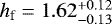 . This would be an unprecedented constraint on the Love number of an exoplanet which would give us strong insights into the interior of these planets and their similarities and differences with the Solar System giants.
5.4 Measuring the Love number from planet–planet interaction
HAT-P-13 b is the only exoplanet for which the measurement of the Love number was confirmed. For HAT-P-13 b, the determination of the Love number was made by an alternative method through the fixed point orbital eccentricity (Batygin et al. 2009; Kramm et al. 2012; Buhler et al. 2016). This method, proposed byBatygin et al. (2009), is based on dynamical effects, and thus accesses the potential Love number, kf, instead of the radial Love number, hf, as in our case. The two Love numbers are related to each other by hf = 1 + kf (e.g. Lambeck 1980), but while hf solely depends on the shape of the planet, kf depends on the knowledge of all dynamical effects in the system that can disturb the precession rate. It is, therefore, a much less direct method.
Measuring the hf directly from the signature in the light curve only assumes that the orbit of the planet is circular and its rotation synchronous (Correia 2014). These two hypotheses are very likely for planets near the Roche limit. In contrast, many more assumptions are required to measure kf because the precession rate depends on many physical effects, namely general relativity, rotational flattening of both the star and the planet, tidal deformation of both the star and planet, and secular perturbations from all the remaining planets in the system.
Batygin et al. (2009) applied their method to the HAT-P-13 system, which is the only system currently known that fulfils the criteria of applicability. However, some assumptions were necessary for the derivation of the Love number. The most important are coplanar orbits, the eccentricity is locked in a fixed point, and a hierarchical two-planet system. These assumptions are consistent with current observations of the HAT-P-13 system, although they cannot be completely confirmed. If any one of the assumption fails, the measurement of the Love number of HAT-P-13 b would be biased. Nevertheless, the estimate of the Love number has allowed Batygin et al. (2009), Kramm et al. (2012), and Buhler et al. (2016) to place unprecedented constrains on the core mass and on the metallicity of the planet’s envelop, showing the potential of the Love number to lift degenerancies of the interior structure models. Csizmadia et al. (2019) applied the same method to WASP-18Ab deriving a Love number of 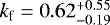 . However, in this case, the cause of the orbital precession is not clear.
In conclusion, the apsidal precession method allows one to derive precise values for the potential fluid Love number for two planet systems with special orbital configuration. However, the several assumptions of the model can have an impact on the accuracy of the measurements of the Love number.
6 Conclusions
We obtained 12 new high-precision transit observations of WASP-103b with the CHEOPS satellite to study the tidal interaction with its host star. The CHEOPS data were analysed with a multi-dimensional GP constrained by several instrumental parameters to correct the systematic effects due to the rotation of the field. We find that the roll angle, which measures the rotation of the field, is the instrumental parameter with higher correlation with the systematic effects. We also found that detrending the data with only the roll angle gives a good correction of the systematic noise. However, in most cases, including other instrumental parameters is a better model of the systematic noise according to Bayesian model comparison.
We find that a linear ephemeris is the preferred model for the orbital evolution of WASP-103b. However, there is a hint of an orbital period increase, contrary to what was expected if tidal decay was dominating the orbital period evolution of this planet. We explored scenarios that could explain a positive period derivative in case it is confirmed by future observations.
One possibility is RV acceleration due to a bound companion. If the known visual companion of WASP-103 is bound, it could affect the transit times of WASP-103b. To check this, we obtained further RV observations with CORALIE and lucky imaging observations with the AstroLux camera. The RV observations are compatible with both a bound companion and a non-bound companion. We find an RV offset of 14 ± 45 m s−1 between the previous observations and the new observations spanning 8 yr. This measured RV offset includes an unknown instrumental offset of 14–24 m s−1 and the hypothetical contribution from a bound companion. The value of the RV offset does not exclude that the visual companion is bound since the RV variations over the 8 yr timescale of the observations are expected to be less than 23.2 ± 3.3 m s−1. Although the RV required to cause the observed transit timing variations by the change in the light travel time is much higher (342 ± 146 m s−1), its high uncertainty also does not allow for the exclusion of this possibility.
The new lucky imaging observations do not find the stellar companion despite the high sensitivity at the position it was observed before. To avoid detection, the companion star had to move in the direction of WASP-103 by 77 au, which is too large for a bound object. Therefore, the new lucky imaging observations support the idea that the visual companion is not bound unless unknown systematics have affected our results. Hence, our data support a non-bound companion, but we recommend further observationsto confirm these results. Long-term monitoring of the RVs, as well as the new data release from Gaia, can help constrain the visual companion. Furthermore, high resolution imaging would allow confirmation of the position of the visual companion and its unbound nature.
Other possibilities to explain a positive period derivative are the Applegate effect and apsidial precession. However, a simpler explanation would be statistical artefacts. Several systematic effects have been shown to affect the measurement from transit times in exoplanets (e.g. Barros et al. 2013, 2020). Hence, statistical artefacts could cause the measured period to appear to be increasing. This is supported by the Bayesian evidence and a decrease in the measured period derivative Ṗ = 3.6 ± 1.6 × 10⁻¹⁰ relative to previous observations(Ṗ = 8.4 ± 4.0 × 10⁻¹⁰; Patra et al. 2020). If we assume tidal decay is dominating the period evolution of WASP-103b, we can place a lower limit on the tidal quality factor  of 3.3 × 10⁶ at 3 σ, corresponding to a 99.7% confidence interval. This is similar to the recent limit on
  obtained for WASP-18b 3.9 × 10⁶ at a 95% confidence interval (Maciejewski et al. 2020). For these systems, longer monitoring of the transit times will be required in order to constrain the stellar tidal quality factor.
We combined our new 12 CHEOPS light curves with previous transit light curves obtained by HST and Spitzer to measure the deformation of WASP-103b via its Love number. We re-reduced the light curves obtained with HST and Spitzer to correct for systematic effects since corrected light curves were not available in the literature. We measured the tidal deformation of the planet directly from its distortion of the transit light curve. We estimated the Love number of WASP-103b to be  , which is the first 3 σ detection of an exoplanet Love number measured directly from its deformed transit shape.
The Love number of WASP-103b is similar to Jupiter’s and slightly larger than Saturn’s (hf = 1.39 ± 0.024; Lainey et al. 2017). For a given planetary mass and radius, higher Love numbers imply a metal enrichment of the envelope and hence a decrease in the core mass. Our measurement of the Love number can be used to remove degeneracies in planetary internal models, allowing one to calculate the core size and the composition of WASP-103b (Baumeister et al. 2020). Uncertainties in the limb darkening can influence the measurement of the Love number and hence we have performed a careful treatment of the limb darkening and several tests that indicate that our results are robust.
Future observations with the JWST can help to better constrain the Love number of WASP-103b and gain an unprecedented view of the interior of this hot Jupiter. This could help us to better understand these extreme systems.
Acknowledgements
CHEOPS is an ESA mission in partnership with Switzerland with important contributions to the payload and the ground segment from Austria, Belgium, France, Germany, Hungary, Italy, Portugal, Spain, Sweden, and the United Kingdom. The CHEOPS Consortium would like to gratefully acknowledge the support received by all the agencies, offices, universities, and industries involved. Their flexibility and willingness to explore new approaches were essential to the success of this mission. This work was supported by FCT – Fundação para a Ciência e a Tecnologia through national funds and by FEDER through COMPETE2020 – Programa Operacional Competitividade e Internacionalizacão by these grants: UID/FIS/04434/2019, UIDB/04434/2020, UIDP/04434/2020, PTDC/FIS-AST/32113/2017 and POCI-01-0145-FEDER- 032113, PTDC/FIS-AST/28953/2017 and POCI-01-0145-FEDER-028953, PTDC/FIS-AST/28987/2017 and POCI-01- 0145-FEDER-028987, UIDB/04564/2020 UIDP/04564/2020, PTDC/FIS-AST/7002/2020, POCI-01-0145-FEDER-022217, POCI-01-0145-FEDER-029932. O.D.S.D. is supported in the form of work contract (DL 57/2016/CP1364/CT0004) funded by national funds through FCT. S.G.S. acknowledges support from FCT through FCT contract nr. CEECIND/00826/2018 and POPH/FSE (EC). M.J.H. and Y.A. acknowledge the support of the Swiss National Fund under grant 200020_172746. S.H. gratefully acknowledges CNES funding through the grant 837319. D.K. acknowledges partial financial support from the Center for Space and Habitability (CSH), the PlanetS National Center of Competence in Research (NCCR), and the Swiss National Science Foundation and the Swiss-based MERAC Foundation. A.C.C. and T.G.W. acknowledge support from STFC consolidated grant number ST/M001296/1. P.M. acknowledges support from STFC research grant number ST/M001040/1. This work was also partially supported by a grant from the Simons Foundation (PI Queloz, grant number 327127). B.-O.D. acknowledges support from the Swiss National Science Foundation (PP00P2-190080). ABr was supported by the SNSA. We acknowledge support from the Spanish Ministry of Science and Innovation and the European Regional Development Fund through grants ESP2016-80435-C2-1-R, ESP2016-80435-C2-2-R, PGC2018-098153-B-C33, PGC2018-098153-B-C31, ESP2017-87676-C5-1-R, MDM-2017-0737 Unidad de Excelencia Maria de Maeztu-Centro de Astrobiologí a (INTA-CSIC), as well as the support of the Generalitat de Catalunya/CERCA programme. The MOC activities have been supported by the ESA contract no. 4000124370. X.B., S.C., D.G., M.F., and J.L. acknowledge their roles as ESA-appointed CHEOPS science team members. This project was supported by the CNES. The Belgian participation to CHEOPS has been supported by the Belgian Federal Science Policy Office (BELSPO) in the framework of the PRODEX programme, and by the University of Liège through an ARC grant for Concerted Research Actions financed by the Wallonia-Brussels Federation. This project has received funding from the European Research Council (ERC) under the European Union’s Horizon 2020 research and innovation programme (project FOUR ACESgrant agreement no. 724427). C.M.P. and M.F. gratefully acknowledge the support of the Swedish National Space Agency (DNR 65/19, 174/18). DG gratefully acknowledges financial support from the Cassa di Risparmio di Torino (CRT) foundation under Grant No. 2018.2323 “Gaseous or rocky? Unveiling the nature of small worlds”. M.G. is an F.R.S.-FNRS Senior Research Associate. KGI is the ESA CHEOPS Project Scientist and is responsible for the ESA CHEOPS Guest Observers Programme. She does not participate in, or contribute to, the definition of the Guaranteed Time Programme of the CHEOPS mission through which observations described in this paper have been taken, nor to any aspect of target selection for the programme. She acknowledges support from the Spanish Ministry of Science and Innovation and the European Regional Development Fund through grant PGC2018-098153-B-C33, as well as the support of the Generalitat de Catalunya/CERCA programme. This project has been supported by the Hungarian National Research, Development and Innovation Office (NKFIH) grants GINOP-2.3.2-15-2016-00003, K-119517, K-125015, and the City of Szombathely under Agreement No. 67.177-21/2016. V.V.G. is an F.R.S.-FNRS Research Associate. J.L.-B. acknowledges financial support received from “la Caixa” Foundation (ID 100010434) and from the European Union’s Horizon 2020 research and innovation programme under the Marie Skłodowska-Curie grant agreement no. 847648, with fellowship code LCF/BQ/PI20/11760023. Based on observationscollected at Centro Astronómico Hispano en Andalucía (CAHA) at Calar Alto, operated jointly by Instituto de Astrofísica de Andalucía (CSIC) and Junta de Andalucía. G.B. acknowledges support from CHEOPS ASI-INAF agreement no. 2019-29-HH.0. M.L. acknowledges support from the Swiss National Science Foundation under Grant No. PCEFP2 194576. A.De. acknowledges the financial support of the European Research Council (ERC) under the European Union’s Horizon 2020 research and innovation programme (project FOUR ACES; grant agreement no. 724427). A.De. also acknowledges financial support of the Swiss National Science Foundation (SNSF) through the National Centre for Competence in Research “PlanetS”. L.D. is an F.R.S.-FNRS Postdoctoral Researcher. We thank Daniel Foreman-Mackey for his insight into model comparison versus parameter inference.
Appendix A Figures of the lucky imaging observations
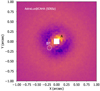 |
Fig. A.1 AstraLux high-spatial resolution image of WASP-103 obtained on 13 January 2021 in the SDSSz bandpass. The image corresponds to the stacking of the 10% frames with the highest Strehl ratio. We removed a fitted PSF of the main target as a combination of a Gaussian and a Lorentzian profile. The location of the previously detected companion by Ngo et al. (2016) is marked as ’B?’. |
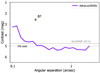 |
Fig. A.2 Sensitivity curve for the AstraLux image of WASP-103. The 1% contamination level is marked by the horizontal dotted line and the maximum magnitude of a blended binary to be able to mimic the transit of WASP-103b is marked by the horizontal dashed line. The location of the previously detected companion by Ngo et al. (2016) is marked as a star-like symbol. |
Appendix B Priors for the limb darkening coefficients
Priors for LD coefficients for the quadratic law.
Priors for LD coefficients for the non-linear law.
References
- Akinsanmi, B., Barros, S. C. C., Santos, N. C., et al. 2019, A&A, 621, A117 [NASA ADS] [CrossRef] [EDP Sciences] [Google Scholar]
- Ambikasaran, S., Foreman-Mackey, D., Greengard, L., Hogg, D. W., & O’Neil, M. 2015, IEEE Trans. Pattern Anal. Mach. Intell., 38, 252 [Google Scholar]
- Applegate, J. H. 1992, ApJ, 385, 621 [Google Scholar]
- Barnes, S. A. 2010, ApJ, 722, 222 [Google Scholar]
- Barnes, J. W., & Fortney, J. J. 2003, ApJ, 588, 545 [NASA ADS] [CrossRef] [Google Scholar]
- Barros, S. C. C., Boué, G., Gibson, N. P., et al. 2013, MNRAS, 430, 3032 [NASA ADS] [CrossRef] [Google Scholar]
- Barros, S. C. C., Demangeon, O., Díaz, R. F., et al. 2020, A&A, 634, A75 [EDP Sciences] [Google Scholar]
- Batygin, K., Bodenheimer, P., & Laughlin, G. 2009, ApJ, 704, L49 [NASA ADS] [CrossRef] [Google Scholar]
- Baumeister, P., Padovan, S., Tosi, N., et al. 2020, ApJ, 889, 42 [Google Scholar]
- Benz, W., Broeg, C., Fortier, A., et al. 2021, Exp. Astron., 51, 109 [Google Scholar]
- Blackwell, D. E., & Shallis, M. J. 1977, MNRAS, 180, 177 [NASA ADS] [CrossRef] [Google Scholar]
- Bonfanti, A., & Gillon, M. 2020, A&A, 635, A6 [NASA ADS] [CrossRef] [EDP Sciences] [Google Scholar]
- Bonfanti, A., Ortolani, S., Piotto, G., & Nascimbeni, V. 2015, A&A, 575, A18 [NASA ADS] [CrossRef] [EDP Sciences] [Google Scholar]
- Bonfanti, A., Ortolani, S., & Nascimbeni, V. 2016, A&A, 585, A5 [NASA ADS] [CrossRef] [EDP Sciences] [Google Scholar]
- Bonfanti, A., Delrez, L., Hooton, M. J., et al. 2021, A&A, 646, A157 [EDP Sciences] [Google Scholar]
- Bouma, L. G., Winn, J. N., Baxter, C., et al. 2019, AJ, 157, 217 [NASA ADS] [CrossRef] [Google Scholar]
- Bruno, G., Lewis, N. K., Stevenson, K. B., et al. 2018, AJ, 155, 55 [NASA ADS] [CrossRef] [Google Scholar]
- Budaj, J. 2011, AJ, 141, 59 [NASA ADS] [CrossRef] [Google Scholar]
- Buhler, P. B., Knutson, H. A., Batygin, K., et al. 2016, ApJ, 821, 26 [CrossRef] [Google Scholar]
- Burton, J. R., Watson, C. A., Fitzsimmons, A., et al. 2014, ApJ, 789, 113 [NASA ADS] [CrossRef] [Google Scholar]
- Cartier, K. M. S., Beatty, T. G., Zhao, M., et al. 2017, AJ, 153, 34 [Google Scholar]
- Castelli, F., & Kurucz, R. L. 2003, in IAU Symposium, 210, Modelling of Stellar Atmospheres, eds. N. Piskunov, W. W. Weiss, & D. F. Gray, A20 [NASA ADS] [Google Scholar]
- Claret, A. 2000, A&A, 363, 1081 [NASA ADS] [Google Scholar]
- Collier Cameron, A., & Jardine, M. 2018, MNRAS, 476, 2542 [Google Scholar]
- Correia, A. C. M. 2014, A&A, 570, L5 [NASA ADS] [CrossRef] [EDP Sciences] [Google Scholar]
- Correia, A. C. M., & Rodríguez, A. 2013, ApJ, 767, 128 [NASA ADS] [CrossRef] [Google Scholar]
- Csizmadia, S., Pasternacki, T., Dreyer, C., et al. 2013, A&A, 549, A9 [NASA ADS] [CrossRef] [EDP Sciences] [Google Scholar]
- Csizmadia, S., Hellard, H., & Smith, A. M. S. 2019, A&A, 623, A45 [NASA ADS] [CrossRef] [EDP Sciences] [Google Scholar]
- Delrez, L., Madhusudhan, N., Lendl, M., et al. 2018, MNRAS, 474, 2334 [NASA ADS] [CrossRef] [Google Scholar]
- Demangeon, O. D. S., Faedi, F., Hébrard, G., et al. 2018, A&A, 610, A63 [NASA ADS] [CrossRef] [EDP Sciences] [Google Scholar]
- Demangeon, O. D. S., Zapatero Osorio, M. R., Alibert, Y., et al. 2021, A&A, 653, A41 [NASA ADS] [CrossRef] [EDP Sciences] [Google Scholar]
- Deming, D., Wilkins, A., McCullough, P., et al. 2013, ApJ, 774, 95 [Google Scholar]
- Demory, B.-O., Gillon, M., de Wit, J., et al. 2016a, Nature, 532, 207 [NASA ADS] [CrossRef] [Google Scholar]
- Demory, B.-O., Queloz, D., Alibert, Y., Gillen, E., & Gillon, M. 2016b, ApJ, 825, L25 [NASA ADS] [CrossRef] [Google Scholar]
- Díaz, R. F., Almenara, J. M., Santerne, A., et al. 2014, MNRAS, 441, 983 [Google Scholar]
- Durante, D., Parisi, M., Serra, D., et al. 2020, Geophys. Res. Lett., 47, e86572 [NASA ADS] [CrossRef] [Google Scholar]
- Eastman, J., Siverd, R., & Gaudi, B. S. 2010, PASP, 122, 935 [Google Scholar]
- Espinoza, N., & Jordán, A. 2015, MNRAS, 450, 1879 [Google Scholar]
- Ferraz-Mello, S., Rodríguez, A., & Hussmann, H. 2008, Celest. Mech. Dyn. Astron., 101, 171 [Google Scholar]
- Foreman-Mackey, D., Hogg, D. W., Lang, D., & Goodman, J. 2013, PASP, 125, 306 [Google Scholar]
- Fulton, B. J., Petigura, E. A., Blunt, S., & Sinukoff, E. 2018, PASP, 130, 044504 [Google Scholar]
- Gaia Collaboration (Brown, A. G. A., et al.) 2018, A&A, 616, A1 [NASA ADS] [CrossRef] [EDP Sciences] [Google Scholar]
- Gaia Collaboration (Brown, A. G. A., et al.) 2021, A&A, 649, A1 [NASA ADS] [CrossRef] [EDP Sciences] [Google Scholar]
- Gillon, M., Triaud, A. H. M. J., Fortney, J. J., et al. 2012, A&A, 542, A4 [NASA ADS] [CrossRef] [EDP Sciences] [Google Scholar]
- Gillon, M., Anderson, D. R., Collier-Cameron, A., et al. 2014, A&A, 562, L3 [NASA ADS] [CrossRef] [EDP Sciences] [Google Scholar]
- Gillon, M., Triaud, A. H. M. J., Demory, B.-O., et al. 2017, Nature, 542, 456 [NASA ADS] [CrossRef] [Google Scholar]
- Goodman, J., & Weare, J. 2010, Commun. Appl. Math. Comput. Sci., 5, 65 [Google Scholar]
- Hellard, H., Csizmadia, S., Padovan, S., et al. 2019, ApJ, 878, 119 [NASA ADS] [CrossRef] [Google Scholar]
- Hestroffer, D. 1997, A&A, 327, 199 [NASA ADS] [Google Scholar]
- Higson, E., Handley, W., Hobson, M., & Lasenby, A. 2019, Stat. Comput., 29, 891 [Google Scholar]
- Hormuth, F., Hippler, S., Brandner, W., Wagner, K., & Henning, T. 2008, Ground-based and Airborne Instrumentation for Astronomy II [Google Scholar]
- Howarth, I. D. 2011, MNRAS, 413, 1515 [NASA ADS] [CrossRef] [Google Scholar]
- Hoyer, S., Guterman, P., Demangeon, O., et al. 2020, A&A, 635, A24 [NASA ADS] [CrossRef] [EDP Sciences] [Google Scholar]
- Husser, T.-O., Wende-von Berg, S., Dreizler, S., et al. 2013, A&A, 553, A6 [NASA ADS] [CrossRef] [EDP Sciences] [Google Scholar]
- Hut, P. 1980, A&A, 92, 167 [NASA ADS] [Google Scholar]
- Ingalls, J. G., Krick, J. E., Carey, S. J., et al. 2016, AJ, 152, 44 [NASA ADS] [CrossRef] [Google Scholar]
- Kass, R. E., & Raftery, A. E. 1995, J. Am. Stat. Assoc., 90, 773 [Google Scholar]
- Kipping, D. M. 2013a, MNRAS, 435, 2152 [Google Scholar]
- Kipping, D. M. 2013b, MNRAS, 434, L51 [Google Scholar]
- Kopal, Z. 1950, Harvard College Observatory Circular, 454, 1 [NASA ADS] [Google Scholar]
- Kramm, U., Nettelmann, N., Redmer, R., & Stevenson, D. J. 2011, A&A, 528, A18 [NASA ADS] [CrossRef] [EDP Sciences] [Google Scholar]
- Kramm, U., Nettelmann, N., Fortney, J. J., Neuhäuser, R., & Redmer, R. 2012, A&A, 538, A146 [NASA ADS] [CrossRef] [EDP Sciences] [Google Scholar]
- Kreidberg, L. 2015, PASP, 127, 1161 [Google Scholar]
- Kreidberg, L., Line, M. R., Parmentier, V., et al. 2018, AJ, 156, 17 [NASA ADS] [CrossRef] [Google Scholar]
- Lainey, V., Jacobson, R. A., Tajeddine, R., et al. 2017, Icarus, 281, 286 [Google Scholar]
- Lambeck, K. 1980, The earth’s variable rotation: geophysical causes and consequences [CrossRef] [Google Scholar]
- Lanotte, A. A., Gillon, M., Demory, B. O., et al. 2014, A&A, 572, A73 [NASA ADS] [CrossRef] [EDP Sciences] [Google Scholar]
- Lanza, A. F., Rodono, M., & Rosner, R. 1998, MNRAS, 296, 893 [Google Scholar]
- Leconte, J., Lai, D., & Chabrier, G. 2011, A&A, 528, A41 [NASA ADS] [CrossRef] [EDP Sciences] [Google Scholar]
- Lendl, M., Ehrenreich, D., Turner, O. D., et al. 2017, A&A, 603, L5 [NASA ADS] [CrossRef] [EDP Sciences] [Google Scholar]
- Lillo-Box, J., Barrado, D., & Bouy, H. 2012, A&A, 546, A10 [NASA ADS] [CrossRef] [EDP Sciences] [Google Scholar]
- Lillo-Box, J., Barrado, D., & Bouy, H. 2014, A&A, 566, A103 [NASA ADS] [CrossRef] [EDP Sciences] [Google Scholar]
- Lindegren, L., Bastian, U., Biermann, M., et al. 2021, A&A, 649, A4 [EDP Sciences] [Google Scholar]
- Love, A. E. H. 1911, Some Problems of Geodynamics [Google Scholar]
- Luger, R., Foreman-Mackey, D., & Hogg, D. W. 2017, Res. Notes Am. Astron. Soc., 1, 7 [Google Scholar]
- Maciejewski, G., Dimitrov, D., Fernández, M., et al. 2016, A&A, 588, L6 [NASA ADS] [CrossRef] [EDP Sciences] [Google Scholar]
- Maciejewski, G., Fernández, M., Aceituno, F., et al. 2018, Acta Astron., 68, 371 [NASA ADS] [Google Scholar]
- Maciejewski, G., Knutson, H. A., Howard, A. W., et al. 2020, Acta Astron., 70, 1 [NASA ADS] [Google Scholar]
- Mandel, K., & Agol, E. 2002, ApJ, 580, L171 [Google Scholar]
- Marigo, P., Girardi, L., Bressan, A., et al. 2017, ApJ, 835, 77 [Google Scholar]
- Maxted, P. F. L. 2016, A&A, 591, A111 [NASA ADS] [CrossRef] [EDP Sciences] [Google Scholar]
- Maxted, P. F. L., & Gill, S. 2019, A&A, 622, A33 [NASA ADS] [CrossRef] [EDP Sciences] [Google Scholar]
- Maxted, P. F. L., Ehrenreich, D., Wilson, T. G., et al. 2021, MNRAS, in press, [arXiv:2111.08828] [Google Scholar]
- Meibom, S., & Mathieu, R. D. 2005, ApJ, 620, 970 [Google Scholar]
- Mendonça, J. M., Malik, M., Demory, B.-O., & Heng, K. 2018, AJ, 155, 150 [Google Scholar]
- Mordasini, C., Alibert, Y., Klahr, H., & Henning, T. 2012, A&A, 547, A111 [NASA ADS] [CrossRef] [EDP Sciences] [Google Scholar]
- Morello, G., Tsiaras, A., Howarth, I. D., & Homeier, D. 2017, AJ, 154, 111 [NASA ADS] [CrossRef] [Google Scholar]
- Murray, C. D., & Dermott, S. F. 1999, Solar system dynamics [Google Scholar]
- Ngo, H., Knutson, H. A., Hinkley, S., et al. 2016, ApJ, 827, 8 [Google Scholar]
- Ogilvie, G. I., & Lin, D. N. C. 2004, ApJ, 610, 477 [Google Scholar]
- Ogilvie, G. I., & Lin, D. N. C. 2007, ApJ, 661, 1180 [Google Scholar]
- Parviainen, H., & Aigrain, S. 2015, MNRAS, 453, 3821 [Google Scholar]
- Patra, K. C., Winn, J. N., Holman, M. J., et al. 2017, AJ, 154, 4 [Google Scholar]
- Patra, K. C., Winn, J. N., Holman, M. J., et al. 2020, AJ, 159, 150 [NASA ADS] [CrossRef] [Google Scholar]
- Penev, K., & Sasselov, D. 2011, ApJ, 731, 67 [NASA ADS] [CrossRef] [Google Scholar]
- Pepe, F., Mayor, M., Galland, F., et al. 2002, A&A, 388, 632 [NASA ADS] [CrossRef] [EDP Sciences] [Google Scholar]
- Phinney, E. S. 1992, Philos. Trans. R. Soc. Lond. A, 341, 39 [NASA ADS] [CrossRef] [Google Scholar]
- Queloz, D., Mayor, M., Weber, L., et al. 2000, A&A, 354, 99 [NASA ADS] [Google Scholar]
- Ragozzine, D., & Wolf, A. S. 2009, ApJ, 698, 1778 [Google Scholar]
- Rasmussen, C. E., & Williams, C. K. I. 2006, Gaussian Processes for Machine Learning (MIT Press) [Google Scholar]
- Salmon, S. J. A. J., Van Grootel, V., Buldgen, G., Dupret, M. A., & Eggenberger, P. 2021, A&A, 646, A7 [NASA ADS] [CrossRef] [EDP Sciences] [Google Scholar]
- Schanche, N., Hébrard, G., Collier Cameron, A., et al. 2020, MNRAS, 499, 428 [NASA ADS] [CrossRef] [Google Scholar]
- Scuflaire, R., Théado, S., Montalbán, J., et al. 2008, Ap&SS, 316, 83 [Google Scholar]
- Seager, S., & Hui, L. 2002, ApJ, 574, 1004 [NASA ADS] [CrossRef] [Google Scholar]
- Short, D. R., Welsh, W. F., Orosz, J. A., Windmiller, G., & Maxted, P. F. L. 2019, Res. Notes AAS, 3, 117 [NASA ADS] [CrossRef] [Google Scholar]
- Skilling, J. 2012, in AIP Conf. Ser., 1443, Bayesian Inference and Maximum Entropy Methods in Science and Engineering: 31st International Workshop on Bayesian Inference and Maximum Entropy Methods in Science and Engineering, eds. P. Goyal, A. Giffin, K. H. Knuth, & E. Vrscay, 145 [NASA ADS] [Google Scholar]
- Skilling, J. 2004, in AIP Conf. Ser., 735, Bayesian Inference and Maximum Entropy Methods in Science and Engineering: 24th International Workshop on Bayesian Inference and Maximum Entropy Methods in Science and Engineering, eds. R. Fischer, R. Preuss, & U. V. Toussaint, 395 [NASA ADS] [CrossRef] [Google Scholar]
- Skrutskie, M. F., Cutri, R. M., Stiening, R., et al. 2006, AJ, 131, 1163 [NASA ADS] [CrossRef] [Google Scholar]
- Sousa, S. G., Adibekyan, V., Delgado-Mena, E., et al. 2018, A&A, 620, A58 [NASA ADS] [CrossRef] [EDP Sciences] [Google Scholar]
- Southworth, J., Mancini, L., Ciceri, S., et al. 2015, MNRAS, 447, 711 [NASA ADS] [CrossRef] [Google Scholar]
- Speagle, J. S. 2020, MNRAS, 493, 3132 [Google Scholar]
- Stevenson, K. B., Harrington, J., Fortney, J. J., et al. 2012, ApJ, 754, 136 [Google Scholar]
- Stevenson, K. B., Désert, J.-M., Line, M. R., et al. 2014, Science, 346, 838 [Google Scholar]
- Turner, J. D., Leiter, R. M., Biddle, L. I., et al. 2017, MNRAS, 472, 3871 [NASA ADS] [CrossRef] [Google Scholar]
- Virtanen, P., Gommers, R., Oliphant, T. E., et al. 2020, Nat. Methods, 17, 261 [Google Scholar]
- Watson, C. A., & Marsh, T. R. 2010, MNRAS, 405, 2037 [NASA ADS] [Google Scholar]
- Wöllert, M., & Brandner, W. 2015, A&A, 579, A129 [NASA ADS] [CrossRef] [EDP Sciences] [Google Scholar]
- Wright, E. L., Eisenhardt, P. R. M., Mainzer, A. K., et al. 2010, AJ, 140, 1868 [Google Scholar]
- Yee, S. W., Winn, J. N., Knutson, H. A., et al. 2020, ApJ, 888, L5 [Google Scholar]
PAdova & TRieste Stellar Evolutionary Code: http://stev.oapd.inaf.it/cgi-bin/cmd
All Tables
Derived transit parameters of WASP-103b for an ellipsoidal planet model and a spherical model.
Comparison of the derived Love number for the individual instruments and their combination.
Comparison of the derived Love number, significance of the detection, and Bayes factors for the three LD laws considered.
All Figures
|
Fig. 1 Top panel: field of view of WASP-103 as observed by CHEOPS transit #10. Bottom panel: field of view of WASP-103 simulated by the DRP based on the Gaia catalogue and excluding WASP-103. The red cross marks the target position, while the red circle shows the DEFAULT aperture. The image scale is 1 arcsec per pixel. |
| In the text | |
|
Fig. 2 Residuals of the transit fit as a function of the roll angle of the satellite for transit number 8. A clear dependence is seen which is well fitted with a non-parametric GP model overplotted in orange (see Sect. 2.3.1). The best fit length scale hyper-parameter in this case was
|
| In the text | |
|
Fig. 3 Left panel: transit light curves of WASP-103b obtained with CHEOPS. We overplot our best fit model that includes a transit model and the GP model to account for systematics dependent on the instrumental parameters. Right panel: residuals of the fit of the transit model and the GP model. For clarity, the errors are only shown in the residuals. The light curves and residuals are offset vertically for clarity. |
| In the text | |
|
Fig. 4 Derived mid-transit times of WASP-103b after removing a linear ephemerides. The CHEOPS data are shown in blue, the re-reduced HST data and Spitzer are shown in magenta, and the previously published times are shown in black. The previously published quadratic ephemerides (Patra et al. 2020) is shown in green with the 1 σ uncertainty limit, while our new result is shown in red. |
| In the text | |
|
Fig. 5 Time folded transit light curves of WASP-103b obtained with Spitzer 1, Spitzer 2, CHEOPS, and HST. The CHEOPS transit light curve is a combination of 12 individual transits, while the HST light curve is a combination of two transits. The best fit ellipsoidal transit model is shown in blue. We also plotted the residuals of the best fit ellipsoidal model (blue) and the best fit spherical model (red) binned to 5 min. On the latter, we overplotted the signature of the deformation(green) which is the difference between the best fit spherical model and the best fit ellipsoidal models. For clarity, we replotted a zoom of the signature of the deformation in the bottom panel for each filter. We also show the mean uncertainties of the original data points and of the binned residuals. |
| In the text | |
|
Fig. 6 Derived correlation plots and posterior probability distributions of the transit parameters of WASP-103b for the spherical (red) and ellipsoidal model (blue). The vertical lines show the median of the distributions and the shaded area shows the 68% confidence intervals. We show the 1 σ (dark blue and dark red) and 2 σ (light blue and light red) contours. We obtained a 3 σ detection of the Love number. The parameter distributions also clearly show that the ellipsoidal model is not as well constrained as the spherical model due to strong correlations between the Love number and the radius ratio. For the ellipsoidal model, the radius ratio refers to the volumetric radius. The superscripts sp1, sp2, ch, and hst refer to the two Spitzer channels, CHEOPS, and HST, respectively. |
| In the text | |
|
Fig. 7 Stellar intensity profiles from the PHOENIX (solid purple line) and ATLAS (solid black line) stellar grids for the HST WFC3.IR.G141 filter as a function of μ
( |
| In the text | |
|
Fig. A.1 AstraLux high-spatial resolution image of WASP-103 obtained on 13 January 2021 in the SDSSz bandpass. The image corresponds to the stacking of the 10% frames with the highest Strehl ratio. We removed a fitted PSF of the main target as a combination of a Gaussian and a Lorentzian profile. The location of the previously detected companion by Ngo et al. (2016) is marked as ’B?’. |
| In the text | |
|
Fig. A.2 Sensitivity curve for the AstraLux image of WASP-103. The 1% contamination level is marked by the horizontal dotted line and the maximum magnitude of a blended binary to be able to mimic the transit of WASP-103b is marked by the horizontal dashed line. The location of the previously detected companion by Ngo et al. (2016) is marked as a star-like symbol. |
| In the text | |
Current usage metrics show cumulative count of Article Views (full-text article views including HTML views, PDF and ePub downloads, according to the available data) and Abstracts Views on Vision4Press platform.
Data correspond to usage on the plateform after 2015. The current usage metrics is available 48-96 hours after online publication and is updated daily on week days.
Initial download of the metrics may take a while.