© ESO 2021

1. Introduction

Blazars are known as the most extreme subclass of active galactic nuclei (AGN), with their relativistic jets pointing towards the observer. Blazar emission is non-thermal, spreading over the entire electromagnetic spectrum, and it is characterized by rapid variability, high optical polarization, and apparent superluminal motion. One of the characteristic features of this emission is the shape of its spectral energy distribution (SED), which usually has two components: a low-energy component extending from radio to UV and soft X-rays and a high-energy one lying between hard X-rays and TeV γ-rays.

Modeling a blazar’s SED implies the existence of a non-thermal population of particles. In many cases, blazar emission is explained by a relativistic electron population that accelerates and radiates inside a spherical region (for more details, see the following review papers: Padovani et al. 2017; Hovatta & Lindfors 2019; Böttcher 2019; Blandford et al. 2019; Matthews et al. 2020). This is the so-called one-zone leptonic model, which has been applied widely in modeling the blazar SED (e.g., Marscher & Gear 1985; Inoue & Takahara 1996; Mastichiadis & Kirk 1997; Kirk et al. 1998; Kirk & Mastichiadis 1999; Kusunose et al. 2000; Böttcher & Chiang 2002; Tramacere et al. 2011; Asano et al. 2014; Finke 2016; Boula et al. 2019a). In this approach, the low-frequency component is related to synchrotron radiation while the higher energy one is tied to inverse Compton scattering. Reproducing the observed SED allows us to obtain physical parameter constraints.

The multi-wavelength monitoring programs are a unique way of probing the conditions in blazar jets and unveiling the physical processes responsible for the blazar’s non-thermal variable emission. High-quality data, such as time lags between radio and γ-ray emission, which are associated with significant correlations between these energy bands, contribute to improving the understanding of blazar anatomy (e.g., Pavlidou et al. 2014; Esposito et al. 2015; Hovatta et al. 2015; Angelakis et al. 2016; Tavani et al. 2018; Liodakis et al. 2019).

Despite this multi-year monitoring effort, there is still no consensus about the location of the high-energy (X-rays and γ-rays) emission in blazar jets. In particular, the rapid variability, which is an identifying property of blazars, suggests that the non-thermal emission is typically produced in regions of the jet with a size ≪1 light day (e.g., Aharonian et al. 2007; Aleksić et al. 2011). Although electron synchrotron radiation produced in this region can explain the optical-to-X-ray part of the photon spectrum, in most of cases, it cannot account for the jet emission at low frequencies (e.g., ν ≤ 10¹⁰ Hz); in such compact emitting regions, synchrotron radiation is typically self-absorbed (e.g.,van der Laan 1969; Ginzburg & Syrovatskii 1969; Pérez-Torres et al. 2001; Kaiser 2006). However, blazar jets are detected up to GHz frequencies having a power-law spectrum (see also Tingay & de Kool 2003; Stawarz et al. 2008; Ghisellini et al. 2017). In order to solve this discrepancy, it has been proposed that the radio emission, in most cases, is not produced in the same region as the γ-ray. The radio-emitting area should be larger to be less opaque to synchrotron self-absorption (Marscher 1980, 2014; Marscher & Gear 1985; Ghisellini et al. 1985; Potter & Cotter 2012; Potter 2018; Boula et al. 2019b). Still, the results of the various monitoring programs raise several questions about the origin of the radio emission of the jets, which in many cases is variable (Hartman et al. 2001; Kharb et al. 2010; Ghirlanda et al. 2011; Arshakian et al. 2012; Myserlis et al. 2018).

Many theoretical studies are based on an idealized model of a conical steady radio jet, while the component that is associated with the variability of the source is related to shock waves that are propagating in the jet (Blandford & Königl 1979; Georganopoulos & Marscher 1998a,b; Katarzyński et al. 2003). Assuming that electrons are accelerated in such shock fronts and are cooled as they move away from it, one gets that the highest-frequency synchrotron component is emitted from a thin layer behind the shock. In contrast, the lower frequency component is produced in a larger volume, simply because the cooling time for higher-energy electrons is less than for the lower-energy ones, Marscher & Gear (1985). Furthermore, this scenario predicts time lags between high-frequency and low-frequency light curves and a specific evolution of the radio spectrum over time. Potter & Cotter (2012), Potter (2018) proposed a model of a ballistic jet with a uniform structure to investigate the relationship between low- and high-energy emission (see also Katarzyński et al. 2003; Hervet et al. 2015; Richter & Spanier 2016; Zacharias et al. 2021).

The goal of this work is to study the relationship between radio and γ-ray activity in blazars and to localize their emission site using a simple framework that allows for a comprehensive search of the parameter space. More specifically, we use a time-dependent numerical code, originally developed to treat the radiative transfer problem in a static spherical geometry (Mastichiadis & Kirk 1995), to compute the emission from an expanding blob of plasma, (see also Zacharias & Wagner 2016; Boula et al. 2019b). This approach allows γ-rays to be produced more efficiently close to the electron acceleration site, whereas radio is produced much later when the blob has expanded enough to become optically thin to synchrotron self-absorption. The numerical code allows us also to study reaccelerating episodes and we show that depending on the distance, this can produce γ-ray flares, which may or may not accompanied by radio flares.

The paper is structured as follows. In Sect. 2, we present our new one-zone expanding model that considers all the leptonic physical processes. In Sect. 3, we show the dependence on the initial parameters of the transition from the optically thick to the optically thin region due to synchrotron self-absorption. This method guides us to localize the onset of radio emission inside the jet. The initial values of the physical quantities of the source play a vital role in the transition from the optically thick to the optically thin region. In Sect. 4, we present a few characteristic examples for the flaring activity of blazars by assuming electron accelerating episodes and following their evolution. We also apply our model to the flaring episode of Mrk421 that occurred in 2013, explaining the time-lag between γ-ray and radio emission. In Sect. 5, we discuss our results. Finally, in Sect. 6, we give the basic conclusions of our work.

2. One-zone expanding blob model

We consider a blazar with a conical jet whose axis forms an angle of θ_obs to our line of sight. We assume that due to some accelerating episode, relativistic electrons are injected in a spherical region, which we refer to as the “blob” of an initial radius $R_0^{\prime }$.

The blob moves along the jet axis with a velocity of u_Γ = β_Γc ≃ c, corresponding to a Lorentz factor $\mathrm{\Gamma }={(1-{\beta }_{\mathrm{\Gamma }}^2)}^{-1/2}$ and a Doppler factor of δ = [Γ(1 − β_Γ cos θ_obs)]⁻¹. At the same time, it expands in a spherically symmetric way with velocity u_exp in its rest frame. Therefore, if we denote t′ the time as measured in the rest frame of the blob¹, then for its instantaneous radius, following Boula et al. (2019b), we have:

$$\begin{array}{c}\hfill R^{\prime }(t^{\prime })=R_0^{\prime }+u_{\exp }(t^{\prime }-t_0^{\prime }),\end{array}$$(1)

where $t_0^{\prime }$ is the time of the blob formation. Similarly, the instantaneous distance, z, of the blob along the jet at the observer’s frame is given by:

$$\begin{array}{c}\hfill z(t)=z_0+{\beta }_{\mathrm{\Gamma }}c\mathrm{\Gamma }(t^{\prime }-t_0^{\prime }),\end{array}$$(2)

or

$$\begin{array}{c}\hfill z(t)=z_0+{\beta }_{\mathrm{\Gamma }}c\mathrm{\Gamma }[R^{\prime }-R_0^{\prime }]/u_{\exp },\end{array}$$(3)

where z₀ is the blob’s initial distance from the central object. Therefore both quantities, R′ and z, are functions of the time t′.

In order to calculate the electron evolution inside the blob, one needs to take into account, as in the standard leptonic model, synchrotron and inverse Compton losses. However, in the present case, adiabatic losses should also explicitly be taken into account due to the expansion of the blob. We should also consider the possibility that the magnetic field inside the blob might change over time (or radius) for the same reason, affecting the synchrotron losses. Therefore, we parametrize the magnetic field B′ as

$$\begin{array}{c}\hfill B^{\prime }(R^{\prime })=B_0^{\prime }{\left(\frac{R_0^{\prime }}{R^{\prime }}\right)}^s,\end{array}$$(4)

where $B_0^{\prime }$ is the initial value of the magnetic field and s is a free parameter. For the parameter s, we have 1 ≤ s ≤ 2 from magnetic flux conservation with magnetic-field orientations between the extremes of purely toroidal and purely poloidal fields, respectively.

Similarly, the electron injected power might also be a function of time and we parametrize it as

$$\begin{array}{c}\hfill L_{\mathrm{e}}^{\prime \mathrm{inj}}(R^{\prime })=L_{\mathrm{e},0}^{\prime \mathrm{inj}}{\left(\frac{R_0^{\prime }}{R^{\prime }}\right)}^q,\end{array}$$(5)

where $L_{\text{e},\text{0}}^{\prime \text{inj}}$ is the initial electron power and q is a free parameter².

We have developed a numerical code, based on Mastichiadis & Kirk (1995), to calculate the evolution of the electron and photon distribution function in an expanding spherical source. This code solves two integro-differential equations, each describing the losses or sinks as well as the injection of relativistic electrons and photons in the emitting region. The kinetic equation for the differential, with respect to energy, electron number, N_e, is expressed as:

$$\begin{array}{c}\hfill \frac{\partial N_{\mathrm{e}}(\gamma ,R^{\prime })}{\partial t^{\prime }}+{\displaystyle \sum _i\frac{\partial }{\partial \gamma }{\mathcal{L}}_{\mathrm{e}}^{\mathrm{i}}{N}_{\mathrm{e}}(\gamma ,R^{\prime })+\frac{N_{\mathrm{e}}}{t_{\mathrm{esc},\mathrm{e}}^{\prime }}=\sum _i{Q}_{\mathrm{e}}^{\mathrm{i}}(\gamma ,R^{\prime }).}\end{array}$$(6)

We use ${\mathcal{L}}_{\mathrm{e}}^{\mathrm{i}}$ to denote the loss terms and Q_e to denote the injection terms of relativistic electrons. Also, γ = (1 − u²/c²)^−1/2 the electron Lorentz factor, with u as the electron velocity and $t_{\text{esc},\text{e}}^{\prime }$ as the electron escape timescale. Specifically, for the losses, we have:

$$\begin{array}{c}\hfill {\displaystyle \sum _i\frac{\partial }{\partial \gamma }{\mathcal{L}}_{\mathrm{e}}^{\mathrm{i}}=\frac{\partial }{\partial \gamma }[{\mathcal{L}}_{\mathrm{e}}^{\mathrm{syn}}(\gamma ,R^{\prime })+{\mathcal{L}}_{\mathrm{e}}^{\mathrm{ICS}}(\gamma ,R^{\prime })+{\mathcal{L}}_{\mathrm{e}}^{\mathrm{ad}}(\gamma ,R^{\prime })],}\end{array}$$(7)

where ${\mathcal{L}}_{\mathrm{e}}^{\mathrm{syn}}(\gamma ,R^{\prime }),{\mathcal{L}}_{\mathrm{e}}^{\mathrm{ICS}}(\gamma ,R^{\prime }),{\mathcal{L}}_{\mathrm{e}}^{\mathrm{ad}}(\gamma ,R^{\prime })$ are the loss-rates for synchrotron emission, inverse Compton scattering³, and adiabatic expansion that are given by the expressions:

$$\begin{array}{c}\hfill {\mathcal{L}}_{\mathrm{e}}^{\mathrm{syn}}(\gamma ,R^{\prime })=-{\displaystyle \frac{4}{3}}{\sigma }_{\tau }c\frac{U_{\mathrm{B}}^{\prime }(R^{\prime })}{m_{\mathrm{e}}{c}^2}{\beta }^2{\gamma }^2,\end{array}$$(8)

$$\begin{array}{c}\hfill {\mathcal{L}}_{\mathrm{e}}^{\mathrm{ICS}}(\gamma ,R^{\prime })=-{\displaystyle \frac{4}{3}}{\sigma }_{\tau }c\frac{U_{\mathrm{phot}}^{\prime }(R^{\prime })}{m_{\mathrm{e}}{c}^2}{\beta }^2{\gamma }^2,\end{array}$$(9)

and

$$\begin{array}{c}\hfill {\mathcal{L}}_{\mathrm{e}}^{\mathrm{ad}}(\gamma ,R^{\prime })=-{\displaystyle \frac{u_{\exp }}{R^{\prime }}}\gamma ,\end{array}$$(10)

with β = u/c, $U_{\text{B}}^{\prime }({R^{\prime }}^{})$, and $U_{\text{phot}}^{\prime }(R^{\prime })$, the energy densities in magnetic fields and photon fields, respectively.

The injection of relativistic electrons is given by

$$\begin{array}{c}\hfill {\displaystyle \sum _i{Q}_{\mathrm{e}}^{\mathrm{i}}(\gamma ,R^{\prime })=Q_{\mathrm{e}}^{\mathrm{inj}}(\gamma ,R^{\prime })+Q_{\mathrm{e}}^{\gamma \gamma }(\gamma ,R^{\prime }),}\end{array}$$(11)

where $Q_{\mathrm{e}}^{\mathrm{inj}}(\gamma ,R^{\prime })$ is the injection term of primary accelerated electrons and $Q_{\mathrm{e}}^{\gamma \gamma }(\gamma ,R^{\prime })$ is the injection of the pairs that are created by the photon-photon absoprtion. For the injected electron term $Q_{\mathrm{e}}^{\mathrm{inj}}$, we assume that it is related to the electrons injected power by the relation:

$$\begin{array}{c}\hfill L_{\mathrm{e}}^{\prime \mathrm{inj}}(R^{\prime })={(m_{\mathrm{e}}{c}^2)}^2{\displaystyle {\int }_{{\gamma }_{\min }}^{{\gamma }_{\max }}{Q}_{\mathrm{e}}^{\mathrm{inj}}(\gamma ,R^{\prime })\gamma \mathrm{d}\gamma ,}\end{array}$$(12)

where we have assumed a power-law injection:

$$\begin{array}{c}\hfill Q_{\mathrm{e}}^{\mathrm{inj}}(\gamma ,R^{\prime })=q_{\mathrm{e}}(R^{\prime }){\gamma }^{-p}=q_{\mathrm{e},0}{\left(\frac{R_0^{\prime }}{R^{\prime }}\right)}^q{\gamma }^{-p},{\gamma }_{\min }\le \gamma \le {\gamma }_{\max },\end{array}$$(13)

with γ_min, γ_max the minimum and maximum Lorentz factors of the electron distribution, respectively.

The kinetic equation for the differential, with respect to energy, photon number, N_γ, takes the form:

$$\begin{array}{c}\hfill \frac{\partial N_{\gamma }(x^{\prime },R^{\prime })}{\partial t^{\prime }}+\frac{N_{\gamma }(x^{\prime },R^{\prime })}{t_{\mathrm{cross}}^{\prime }}+{\displaystyle \sum _i{\mathcal{L}}_{\gamma }^{\mathrm{i}}{N}_{\gamma }(x^{\prime },R^{\prime })=\sum _i{Q}_{\gamma }^{\mathrm{i}}(x^{\prime },R^{\prime }),}\end{array}$$(14)

where x is the dimensionless photon frequency, namely, x′=hν′/(m_ec²). Photons escape from the source on the timescale $t_{\mathrm{cross}}^{\prime }={\displaystyle \frac{R^{\prime }}{c}}$, which is the light crossing time of the source at time t′ and it is measured in units of the initial light crossing time:

$$\begin{array}{c}\hfill t_{\mathrm{cross},0}^{\prime }=\frac{R_0^{\prime }}{c}.\end{array}$$(15)

The processes of photon-photon absorption and synchrotron self-absorption contribute to the photon sinks as:

$$\begin{array}{c}\hfill {\displaystyle \sum _i{\mathcal{L}}_{\gamma }^i(x^{\prime },R^{\prime })={\mathcal{L}}_{\gamma }^{\gamma \gamma }(x^{\prime },R^{\prime })+{\mathcal{L}}_{\gamma }^{\mathrm{ssa}}(x^{\prime },R^{\prime }),}\end{array}$$(16)

where ${\mathcal{L}}_{\gamma }^{\gamma \gamma }(x^{\prime },R^{\prime })$ and ${\mathcal{L}}_{\gamma }^{\mathrm{ssa}}(x^{\prime },R^{\prime })$ denote the processes of photon-photon absorption and synchrotron self-absorption⁴ respectively. The photon source function is given by:

$$\begin{array}{c}\hfill {\displaystyle \sum _i{Q}_{\gamma }^{\mathrm{i}}(x^{\prime },R^{\prime })=Q_{\gamma }^{\mathrm{syn}}(x^{\prime },R^{\prime })+Q_{\gamma }^{\mathrm{ICS}}(x^{\prime },R^{\prime })}\end{array}$$(17)

where $Q_{\gamma }^{\mathrm{syn}}(x^{\prime },R^{\prime })$ and $Q_{\gamma }^{\mathrm{ICS}}(x^{\prime },R^{\prime })$ are the terms corresponding to synchrotron⁵ radiation and to inverse Compton scattering, respectively.

Equation (14) by construction calculates the differential number of photons inside the source when its radius is R′. From here, one can calculate the co-moving spectral luminosity (erg/sec/Hz) of the source using:

$$\begin{array}{c}\hfill L_{{\nu }^{\prime }}=\frac{3N_{\gamma }(x^{\prime },R^{\prime })}{t_{\mathrm{cross}}^{\prime }(R^{\prime })}\left(\frac{x^{\prime }{m}_{\mathrm{e}}{c}^2}{h}\right)\end{array}$$(18)

and then calculate the observed flux by imposing the usual Doppler transformations. Therefore, Eq. (14) calculates an instantaneous flux coming from a blob of radius R′.

With regard to checking the numerical scheme presented above, especially as far as the expansion is concerned, the various rates have already been tested, for instance, by Mastichiadis & Kirk (1995) and more recently by Cerruti et al. (2021). Thus, we solve the kinetic equation for the electrons (Eq. (6)) analytically by taking into account only the synchrotron and adiabatic losses and we compare the solution to the results of the code. Figure 1a depicts the electron distribution function in the case of continuous electron injection for a decreasing magnetic field. The electron number constantly increases with time as they continuously accumulate inside the source, while the shape of the distribution changes continuously. At early times the distribution is completely cooled due to strong synchrotron losses, however, at later times, adiabatic losses take over and the cooling break moves progressively to higher energies. The analytical and numerical solutions are identical, with the only difference appearing at high energies since we have not included cutoff effects in our analytical solution. Figure 1b depicts the corresponding photon spectrum, which is calculated numerically. The luminosity decreases with time since cooling becomes less efficient at later times while the spectral turnovers correspond to the electron cooling breaks shown in Fig. 1a.

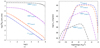Fig. 1. Electron and photon distribution. (a) Plot of the electron energy distribution at different time-steps for synchrotron and adiabatic losses only. The values of the parameters are $R_0^{\prime }={10}^{15}$ cm, $L_{{\mathrm{e}}_0}^{\prime \mathrm{inj}}={10}^{42}$ erg s−1, uexp = 0.1 c, $B_0^{\prime }=100$ G, γmin = 1, γmax = 106, p = 2, and δ = 10, while the profile of magnetic field strength decreases along B′∝R′ − 2 and the electron luminosity is constant in time. Full lines represent analytical solutions, while dashed lines the corresponding numerical ones. (b) Numerical results of the photon SED for the time instances of the depicted electrons.

Figure 2 shows an example when all processes are taken into account in the numerical code. It depicts the time evolution of the SED when the source constantly expands, while the magnetic field strength and the electron injection luminosity decrease with time, that is, q = s = 1. The addition of all processes complicates the evolution over the case of Fig. 1, however, some basic features remain the same. The photon luminosity decreases with time, represented by the color gradient in the logarithmic scale. The SED has two characteristics bumps: the low-frequency component is produced by synchrotron radiation while the higher one is produced due to Synchrotron Self-Compton (SSC). The synchrotron frequency peak is given by the expression ${\nu }_{\mathrm{syn}}^{\prime \mathrm{pk}}\propto B^{\prime }(R^{\prime }){\gamma }_{\max }^2$, so as the magnetic field strength decreases, the peak shifts to lower energies. The same behavior is shown by the Compton peak, which depends both on the energy of synchrotron photons and on γ_max through SSC mechanism. Also, the SSC luminosity decreases quadratically compared to the synchrotron one. Moreover, the spectrum shows a break at radio frequencies due to synchrotron self-absorption, which shifts to lower energies as time increases and the source expands. The slope of the spectrum below the synchrotron self-absorption frequency has the characteristic value of νF_ν ∝ ν^7/2. At all frequencies, the spectral flux peaks at the beginning of the expansion, apart from the radio band which shows a peak at later times. The produced luminosity at these frequencies increases with time, reaching a peak at the transition from the optically thin to the optically thick regime, and then decreases. We expand on this issue in the next section.

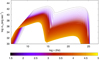Fig. 2. Time evolution of the SED when all the physical processes are taken into account. The parameters have the values: $R_0^{\prime }={10}^{15}$ cm, B0 = 3.16 G, $L_{{\mathrm{e}}_0}^{\prime \mathrm{inj}}={10}^{43}$ erg s−1, $t_{\text{esc},\text{e}}^{\prime }=R^{\prime }/c$, uexp = 0.1 c, γmin = 1, γmax = 104.5, p = 2, and δ = 10. The magnetic field and electron luminosity profiles are ∝R′ − 1. The colorbar refers to time, the time unit is given in days in the co-moving frame and it is on a logarithmic scale.

3. Localization of the onset of radio emission

Very-long-baseline interferometry (VLBI) studies have provided a great deal of information about the structure of the jets and, specifically, about pc-scale jets. As mentioned in the previous section, we can detect radio emission mainly from the regions where the source is optically thin at radio frequencies. In this section, we investigate the role of the expansion velocity on the transition from the optically thick to the optically thin region in the case of an expanding blob (Fig. 3).

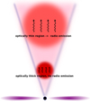Fig. 3. Schematic representation of the one-zone expanding model. The emitting region is optically thick to radio emission close to the central engine. As it propagates along the axis of the jet and expands, it transits to the optically thin region. On the other hand, higher frequencies are emitted from all distances.

In this case, the frequency below which the synchrotron radiation is absorbed can be derived by the condition for the optical depth ${\tau }_{{\nu }_{\text{ssa}}^{\prime }}={\alpha }_{{\nu }_{\text{ssa}}^{\prime }}^{\prime }{R}^{\prime }\backslash 1$, where ${\alpha }_{{\nu }_{\text{ssa}}^{\prime }}^{\prime }({t^{\prime }}^{})$ is the absorption coefficient, for instance, in Eq. (6.53) from Rybicki & Lightman (1979). The synchrotron self-absorption frequency ${\nu }_{\text{ssa}}^{\prime }$ depends on the specifics of the electron distribution and on the magnetic field. In our treatment, both of these depend on the radius of the blob and therefore on the co-moving time (Eqs. (4) and (5)).

Therefore, following the assumptions above, the expression of synchrotron self-absorption for our numerical model takes the form⁶:

$$\begin{array}{c}\hfill {\nu }_{\mathrm{ssa}}^{\prime }(R^{\prime })={\left[k_1{k}_2(p)\frac{L_{\mathrm{e},0}^{\prime \mathrm{inj}}{B}_0^{\prime \frac{p+2}{2}}}{u_{\exp }}\frac{1}{R^{\prime 2}}{\left(\frac{R_0^{\prime }}{R^{\prime }}\right)}^{\frac{s(p+2)}{2}}\right]}^{\frac{2}{p+4}}\end{array}$$

$$\begin{array}{c}\hfill \times \{\begin{array}{cc}{[R_0^{\prime }ln\left(\frac{R^{\prime }}{R_0^{\prime }}\right)]}^{\frac{2}{p+4}}& \mathrm{for}q=1\\ {\left[\frac{R_0^{\prime }}{1-q}[{\left(\frac{R_0^{\prime }}{R^{\prime }}\right)}^{q-1}-1]\right]}^{\frac{2}{p+4}}& \mathrm{for}q\ne 1\end{array},\end{array}$$(19)

where

$$\begin{array}{c}\hfill k_1=\frac{3\sqrt{3}{q}^3}{32{\pi }^2{m}_{\mathrm{e}}}\end{array}$$

and

$$\begin{array}{c}\hfill k_2(p)={\left(\frac{3q}{2\pi m^3{c}^5}\right)}^{\frac{p}{2}}\mathrm{\Gamma }\left(\frac{3p+2}{12}\right)\mathrm{\Gamma }\left(\frac{3p+22}{12}\right){sin}^{\frac{p+2}{2}}\alpha ,\end{array}$$

where Γ(y) is the Gamma function. The luminosity at the synchrotron self-absorption frequency becomes, for instance, as per Stawarz et al. (2008):

$$\begin{array}{c}\hfill {[{\nu }^{\prime }{L}_{\nu }^{\prime }]}_{\mathrm{syn},\mathrm{ssa}}=\frac{c{\sigma }_{\mathrm{T}}}{12\pi m_{\mathrm{e}}{c}^2}\frac{B^{\prime 2}(R^{\prime })}{u_{\exp }}\frac{{\int }_{R_0^{\prime }}^{R^{\prime }}{L}_{\mathrm{e}}^{\prime \mathrm{inj}}(R)\mathrm{d}R}{{\int }_{{\gamma }_{\min }}^{{\gamma }_{\max }}{\gamma }^{1-p}\mathrm{d}\gamma }{\left(\frac{4\pi m_{\mathrm{e}}c{\nu }_{\mathrm{ssa}}^{\prime }(R^{\prime })}{3e{B}^{\prime }(R^{\prime })}\right)}^{\frac{3-p}{2}},\end{array}$$(20)

where σ_T is the Thomson cross-section.

As Eqs. (19) and (20) show, both the synchrotron self-absorption frequency and its corresponding luminosity depend on the initial values and profiles of the key parameters. As we show below, for all physical combinations of these, the source starts self-absorbed and at some point, it becomes transparent. Practically speaking, the distance z_ssa(ν′) at which this occurs marks the onset of radio emission at frequency ν′ and corresponds to the maximum of the lightcurve at that frequency, which can be found from Eq. (2) at a time $t_{\text{ssa}}^{\prime }({\nu }^{\prime })$ defined by ${\tau }_{\text{ssa}}(t_{\text{ssa}}^{\prime }({\nu }^{\prime }))=1$. Therefore for z > z_ssa(ν′) the source is optically thin.

An example of the above can be seen in Fig. 4, which depicts the radio lightcurve at 95 GHz⁷ as a function of time (as measured on Earth) for three different values of the injected electron luminosity in log $L_{\text{e},\text{0}}^{\prime \text{inj}}$ (erg/sec). As we mentioned in Fig. 2, the radio luminosity increases initially with time, it reaches a peak during the transition from the optically thick to the optically thin regime and then decreases. The transition occurs later and is brighter for higher electron luminosities because the number of electrons increases with luminosity. This result is in qualitative agreement with Eqs. (19) and (20). As it turns out, the slopes of the lightcurves depend on the profile of the magnetic field strength (e.g., for B′∝R^{′ − 2} the decay is faster in comparison with B′∝R^{′ − 1}) and of the electron luminosity.

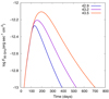Fig. 4. Radio light curves as a function of time as measured in the observer’s frame for various initial values in log $L_{\text{e},\text{0}}^{\prime \text{inj}}$ (erg/sec) of the injected electron luminosity – the injection is assumed to start at t = 0. The other parameters have the values: $R_0^{\prime }={10}^{16.5}$ cm, uexp = 0.05 c, $B_0^{\prime }=1$ G, $t_{\text{esc},\text{e}}^{\prime }=R^{\prime }/c$, γmin = 1, γmax = 106, p = 2, and δ = 10. For the magnetic field profile, we have B′∝R′ − 1 and for the electron luminosity, $L_{\mathrm{e}}^{\prime \mathrm{inj}}\propto R^{\prime -2}$. The source is assumed to be at a distance of 130 Mpc.

Figure 5 depicts the luminosity at 95 GHz as a function of z when all parameters are kept constant except for the expansion velocity (Fig. 5a) and the initial value of the magnetic field (Fig. 5b). Figure 5a shows that as the velocity increases, the transition from the optically thick to the optically thin regime occurs at smaller distances, a result that is expected from Eq. (19). Qualitatively this is to be expected as all the physical quantities change faster; therefore the transition occurs closer to the central engine.

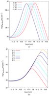Fig. 5. Localization of the onset of the radio emission depending on (a) the expansion velocity in units of c and (b) the initial magnetic field strength, both in logarithmic scale. The other parameters have the values: $R_0^{\prime }={10}^{15}$ cm, $L_{{\mathrm{e}}_0}^{\prime \mathrm{inj}}={10}^{42}$ erg s−1, $t_{\text{esc},\text{e}}^{\prime }=R^{\prime }/c$, γmin = 1, γmax = 106, p = 2, δ = 10 and z0 = 0.001 pc. In sub-figure (a) $B_0^{\prime }=1$ G and in sub-figure (b) uexp = 0.01 c. The profiles of the magnetic field strength and electrons luminosity are decreasing as R−1.

Figure 5b that examines the effects of the blob’s initial magnetic field $B_0^{\prime }$ on the transition distance z_ssa shows that the transition to the optically thin regime occurs at higher distances as $B_0^{\prime }$ increases, while the luminosity during the transition also increases. It is interesting to note that transition occurs around the parsec scale for the most commonly assumed parameters. Finally, we should also mention that we find a very similar behavior if we were to increase, instead of $B_0^{\prime }$, the initial electron luminosity.

4. Simulating flaring episodes in blazars

Blazars are characterized by their variability across the electromagnetic spectrum on time scales from minutes to years. Every flaring episode has its characteristic signature, a fact that makes its modeling a challenge. There are many studies in the literature (e.g., Camenzind & Krockenberger 1992; Wagner & Witzel 1995; Bhatta et al. 2013; Marscher 2014) that are based on the flare’s dependence on the accretion disk and jet plasma variations. Here, we use a simplified way to simulate flaring activity and we present two approaches: radio flares produced due to the expansion of the blob and flares, at all frequencies, produced as a result of particle reaccelerating episodes. In this section, we focus not only on radio flares, but we also examine higher frequencies.

4.1. Flares by energetic blobs

The continuous injection of a series of expanding blobs could create emissions at all values of z. If these blobs had similar initial conditions, then the superposition of their emission at all distances could create a steady-state, quiescent jet (e.g., Potter 2018; Boula et al. 2019b). Supposing that one of the blobs has different initial properties than the rest (which make the steady-state emission), this leads to a disturbance in the emission that will propagate with the particular blob down the jet. In the case where the initial parameters of this disturbance are such that it could lead to higher emission than that of the surrounding blobs, then a flaring episode will ensue and it is possible to calculate the time-dependent emission from it.

According to our analysis in Sect. 2, for conditions where both the electron injection luminosity and the magnetic field drop outwards (i.e., q > 0 and s > 0), the high-energy photons show a peak very early, close to the base of the jet – see Fig. 2. This occurs because the choice of the parameters makes radiation losses more important at the beginning of the expansion. At radio frequencies, however, the peak of the corresponding lightcurve occurs at much larger distances when the blob has reached the region of the transition from the optically thick to the optically thin regime – see Sect. 3. The details of the shape of the radio flare will depend on many parameters, such as the magnetic field strength and the electrons’ power profile on the distance. These parameters, along with the expansion velocity, determine in principle the time-lags between higher frequencies which show a maximum essentially at the base of the jet and the radio frequencies which have their maximum much further out (see also Boula et al. 2019b).

The above can be encoded in Fig. 6, which depicts the distance where the peak of the radio flare occurs as a function of the initial magnetic field value for two magnetic field profiles and two initial electron injections luminosities. The size of the circles scales with the peak radio luminosity at 95 GHz, while the color encodings shows the peak of γ-ray luminosity between 100 MeV and 10 GeV⁸ – we note that the γ-ray peak is not contemporaneous to the peak of the radio flare as it has occurred at earlier times, soon after the injection of the energetic blob.

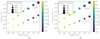Fig. 6. Dependence on initial magnetic field value of the distance where the radio photons escape. The figures depict the two different profiles of the magnetic field strength depending on radius. Also, the peak of γ-ray – at the base of the jet– and the peak of radio luminosity – at the distance where the source becomes optically thin, zssa(95 GHz) = z95 GHz – are represented. The electron power have two different values: (a) $L_{{\mathrm{e}}_0}^{\prime \mathrm{inj}}={10}^{42}$ erg s−1, (b) $L_{{\mathrm{e}}_0}^{\prime \mathrm{inj}}={10}^{43}$ erg s−1. The other parameters have the values: $R_0^{\prime }={10}^{15}$ cm, $t_{\text{esc},\text{e}}^{\prime }=R^{\prime }/c$, uexp = 0.1 c, γmin = 1, γmax = 106, p = 2, δ = 10 and z0 = 0.001 pc. The profile of the electron power follows the magnetic field one.

Several conclusions can be drawn from Fig. 6. Radio flares tend to be more energetic and occur at larger distances along the jet when $B_0^{\prime }$ is higher (results already drawn from Fig. 5b). Furthermore, an anti-correlation between the peak luminosities in γ-ray and radio is found. This is to be expected because for the same injected electron luminosity, higher values of $B_0^{\prime }$ tend to suppress the γ-ray which are produced by the SSC process. Furthermore, the source becomes optically thin at smaller distances when the magnetic field strength and electron power decrease faster with radius. Finally, when the initial power of the injected electrons becomes higher, then all quantities increase but in a slower way than the linear (compare Figs. 6a and b).

4.2. Flares by reaccelerating episodes

An alternative way to produce a flare is to consider a reaccelerating episode in an expanding blob when this is at a certain distance, z_*, from the origin. As in the previous sections, we have not included an acceleration mechanism; instead, we approach this case by increasing the injected power of the relativistic electrons through a Lorentzian function in time:

$$\begin{array}{cc}\hfill Q_{\mathrm{e}}(\gamma ,t^{\prime })& =q_{\mathrm{e}}(t^{\prime }){\gamma }^{-p}(1+\frac{\alpha w^{\prime 2}}{4{(t^{\prime }-t_{\ast }^{\prime })}^2+w^{\prime 2}})\hfill \\ \hfill & =q_{\mathrm{e},0}{\left(\frac{R_0^{\prime }}{R^{\prime }}\right)}^q{\gamma }^{-p}(1+\frac{\alpha w^{\prime 2}}{4{(t^{\prime }-t_{\ast }^{\prime })}^2+w^{\prime 2}}),\hfill \\ \hfill & {\gamma }_{\min }\le \gamma \le {\gamma }_{\max },\hfill \end{array}$$(21)

where α is the value at maximum, w′ the width of the injection, and $t_{*}^{\prime }$ the time of the maximum that corresponds to z_*. The Lorentzian form of the injection is partly motivated by the shape of the pulses that are observed (see also Sikora et al. 2001; Wang & Kusunose 2002).

This assumption allows us to examine the impact of our free parameters, especially the expansion velocity, on the shape of the flares and to study the interplay between radiative and adiabatic losses.

Figure 7 shows the role of u_exp on the pulse shape. Here, all parameters remain constant between cases except of u_exp. The light curves depict the behavior of γ-ray in a reaccelerating episode which occurs at a certain $t_{*}^{\prime }$ that is the same for all cases. This means that episodes with smaller velocities produce flares closer to the origin, where both the magnetic field strength and the electron power are larger. This explains the fact that the γ-ray luminosity is decreasing with increasing u_exp. At the same time, low expansion velocities produce more symmetrical flares because the cooling timescale is $t_{\mathrm{cool}}^{\prime }\ll t_{\mathrm{dyn}}^{\prime }=t_{\mathrm{esc},\mathrm{e}}^{\prime }=\frac{R^{\prime }}{c}$, where $t_{\mathrm{dyn}}^{\prime }$ is the dynamical timescale. On the other hand, fast expansion has a large impact on the cooling timescale because the magnetic field drops substantially as the reaccelerating episode occurs at larger distances and, as a result, the flare appears both asymmetrical and extended.

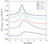Fig. 7. Flares in γ-ray produced by reaccelerating episodes in blobs which have the same initial parameters but different expansion velocities; these are given in units of c in a logarithmic scale. All flaring parameters (see Eq. (21)) are the same. As the velocity increases, the symmetry of the flare breaks as the decay time becomes progressively longer than the rise time producing an extended flare.

The same conclusion can be drawn from Fig. 8. Here, the initial conditions and flaring parameters are identical except for the location of the peak of the reaccelerating episode (see Eq. (21)). The flare that occurs closer to the origin (blue line) is more symmetric than the one that occurs further away (red line), which is dominated by physical escape and adiabatic losses. The second flare is also less bright than the first one, which is another manifestation of this effect.

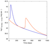Fig. 8. Flares in γ-ray produced by a late reaccelerating episode occurring at distances z1 = 1 pc (blue line) and z2 = 10 pc (red line). The other parameters have the values: $B_0^{\prime }=10$ G, $R_0^{\prime }={10}^{16}$ cm, $L_{{\mathrm{e}}_0}^{\prime \mathrm{inj}}={10}^{44}$ erg s−1, $t_{\text{esc},\text{e}}^{\prime }=R^{\prime }/c$, uexp = 0.1 c, γmin = 1, γmax = 105, p = 2, δ = 10 and the profiles of the magnetic field strength and electrons luminosity are decreasing as R−1. The flaring parameters (see Eq. (21)) are w′ = 100 tcross, 0, and α = 100. The flare which occurs earlier (blue line) is dominated by strong radiation losses, and it appears more symmetrical, contrary to the later one (red line), which is dominated by the adiabatic losses and electron escape.

Radio flares display very different behaviour in these reaccelerating episodes. Contrary to the γ-ray flares, which appear in various shapes and efficiencies, radio frequencies might show no flaring activity at all and this depends critically on the distance where the episode takes place. According to our analysis presented in Sect. 3, a reaccelerating episode will appear in radio only if it occurs beyond the distance where the emission becomes optically thin to synchrotron self-absorption. This is exemplified in Fig. 9, which shows two multiwavelength flares, one induced by electrons injected in an optically thick region (Fig. 9a) and another in an optically thin one (Fig. 9b). We plot the flaring lightcurves (full line) ranging from radio to γ-ray in both figures. For comparison, we also plot the lightcurve we would get without the reaccelerating episode. We can see that when the episode occurs closer to the origin (Fig. 9a), a flare is detected in γ-ray, X-rays, and optical but not in radio frequencies. However, when the episode occurs beyond the transition radius, then a flare appears at all frequencies (Fig. 9b). We note that in radio, higher frequencies appear first.

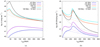Fig. 9. Flares at different wavelengths. (a) Flare in a self-absorbed region. The parameters have the following values: $R_0^{\prime }={10}^{15}$ cm, $B_0^{\prime }=10$ G, $L_{{\mathrm{e}}_0}^{\prime \mathrm{inj}}={10}^{43}$ erg s−1, $t_{\text{esc},\text{e}}^{\prime }=R^{\prime }/c$, uexp = 0.1 c, γmin = 1, γmax = 106, p = 2, δ = 10, and z0 = 0.001 pc. The magnetic field decreases as B′∝R′ − 1 and the electron luminosity as $L_{{\mathrm{e}}_0}^{\prime \mathrm{inj}}\propto R^{\prime -1}$. For the γ-ray flare, we used a pulse which was injected at $t_{*}^{\prime }=100t_{\text{cross},\text{0}}$, with a width w′ = 50 tcross, 0 and α = 45. The dashed lines represent the emission of the blob without the reaccelerating episode; (b) flare in an optically thin region. In this case, we change only the initial electron luminosity $L_{{\mathrm{e}}_0}^{\prime \mathrm{inj}}={10}^{42}$ erg s−1 and the reaccelerating episode occurs at the time, $t_{*}^{\prime }=600t_{\text{cross},\text{0}}$, the rest of the parameters are the same as in case (a).

4.3. Application to the flare of Mrk421

Mrk421 is one of the most well-studied blazars. In April 2013, the source was in intense activity recorded from X-rays to TeV energies. Following this detection the Combined Array for Research in Millimeter-Wave Astronomy (CARMA) observations started. According to Hovatta et al. (2015) the activity of the source in the γ-ray started in March 2013, while the light curve reached its peak on April 14, 2013. The photon flux almost quadrupled within 30 days, while the total activity of the event was about 100 days. In radio frequencies, the intense activity started in April and reached its maximum flux in June with an increase of about a factor of 1.5. In radio frequencies, the source was recorded at 15 GHz and 95 GHz with a slight lag of the two peaks and a complete correlation between them. However, in the data analysis, it appeared that there was also a correlation between γ-ray⁹ and radio.

Motivated by this analysis, we model the observational data as recorded in the 2013 Mrk 421 flaring activity. Our approach to studying this particular flare is to apply the method described earlier in this paper. An energetic plasma blob is produced at a distance z₀ = 0.1 pc from the origin and moves along its axis. The γ-ray (Fig. 10a) are produced by a particle reaccelerating episode at z_* = 0.6 pc through the SSC process. At this distance, the jet is opaque to radio emission due to the synchrotron self-absorption. However, as the plasma blob expands, it becomes optically thin and the radio waves at 95 GHz escape at z_ssa(95 GHz)≃1.1 pc from the origin and this transition is recorded as a flare at the specific frequency (see Fig. 10b). The total electron energy required to power this flare is ∼10⁴⁹ erg. More blobs could explain the rest activity of Mrk421. Despite the fact that the fit is not perfect, it should be compared to a similar fit presented in Fig. 4 of Hovatta et al. (2015), which was obtained using the non-expanding version, Mastichiadis & Kirk (1995) of the present code.

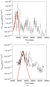Fig. 10. Modeling of Mrk 421 2013 flare. Observational data are presented at Hovatta et al. (2015). The parameter set that we use in this modeling are: $R_0^{\prime }={10}^{16.6}$ cm, $B_0^{\prime }=1.25$ G, $L_{{\mathrm{e}}_0}^{\prime \mathrm{inj}}={10}^{43.2}$ erg s−1, $t_{\text{esc},\text{e}}^{\prime }=R^{\prime }/c$, uexp = 0.05 c, γmin = 1, γmax = 105.1, p = 2, δ = 10 and z0 = 0.1 pc. Magnetic field decreases as B′∝R′ − 1, and electron luminosity as $L_{{\mathrm{e}}_0}^{\prime \mathrm{inj}}\propto R^{\prime -2}$. For the γ-ray flare, we used a pulse that was injected at $t_{*}^{\prime }$ = 40 tcross, 0, with a width w′ = 23 tcross, 0, and α = 60.

5. Discussion

This paper presents an extension of the one-zone leptonic model by including expansion of the source. We have based our numerical scheme on the time-dependent model of Mastichiadis & Kirk (1995), which uses a spherical geometry and has the time and energies of electrons and photons as independent parameters. The present code can describe expansion by replacing the time coordinate with the source’s radius assuming a constant expansion velocity. Therefore, it solves the kinetic equations that describe the evolution of the electron and photon spectra at each source radius or, equivalently, at every measure of distance of the source from the origin.

The kinetic equations are the same as in Mastichiadis & Kirk (1995), with the additions and refinements made in subsequent publications, and describe the usual processes of a one-zone leptonic model, namely, synchrotron and inverse Compton both as energy losses for electrons and sources for photons plus photon-photon interactions both as an injection term for electrons and as a sink term for photons. In addition, we use synchrotron self-absorption for photons and a physical escape term for electrons. Furthermore, the expansion allows us to take explicitly adiabatic losses, which in many non-expanding codes are taken simply as an escape term over the dynamical timescale.

The code, by construction, does not provide a steady-state solution but rather a series of snapshots of the photon spectrum of the source (blob) as it travels down the jet. It also requires more free parameters than the non-expanding model. Thus, we require prescriptions for the profile of the total power injected in electrons and for the magnetic field strength with distance from the origin and a value for the expansion velocity of the blob. These come in addition to the usual parameters of the leptonic model, which include the radius of the blob, its magnetic field strength and the details of the electron injection distribution (total injected power, upper and lower energy cutoffs, and slope in the case of a power-law distribution). Despite the fact that there are ways that to make relations between at least some of these parameters physically (see, e.g., Boula et al. 2019b), for the purpose of the present paper, we used a more generic approach and we have left them as free. We note that we do not vary the shape of the electron distribution (high and low energy cutoffs plus a power-law slope) with the distance because this would have added more free parameters or, alternatively, it would have required a detailed acceleration scheme that we have not included in the present version of the code.

As a first example, we apply the expanding code to treat the radio emission of blazars. This is usually problematic for the non-expanding one-zone models since they provide fits that require a small size for the source and, thus, a high electron number density. This leads, in turn, to an intense synchrotron self-absorption of the radio photons and one requires a different region to produce them (e.g., Marscher 1980; Ghisellini et al. 1985; Marscher & Gear 1985). With the present code, we show that while high-energy photons can be produced close to the base of the jet where the bulk of the injection power takes place, radio photons of some frequency appear when the radius of the blob is such that the optical depth at that particular frequency drops below unity. This occurs at much larger distances from the origin, where the blob has opened up and both the electron density and the magnetic field have dropped. We find that this distance depends on many parameters, but the rule of thumb is that it appears further away from the origin for higher initial values of the electron luminosity and magnetic field strength. If therefore, both of these quantities drop outwards, it is expected that high-energy radiation will be produced very close to the site of the blob formation, while radio photons appear much further away.

We should also emphasize that adiabatic losses can become dominant as the blob expands and this has severe consequences on the radiative efficiency of the electrons; in particular, at large distances from the origin, even freshly injected electrons become inefficient emitters. This can be seen mostly at higher frequencies, even during the duration of a flare. Generally speaking, we find that more asymmetric flares imply high expansion velocities since parameters such as the magnetic field can vary a great deal during an episode of electron injection. Therefore, it is conceivable that, for instance, a γ-ray¹⁰ flare starts when electrons are dominated by radiative losses and ends when they are in the adiabatic phase¹¹. In the non-expanding case, such asymmetries can be achieved only by fine-tuning the electron escape timescale from the source. However, we should mention that we have not considered the light travel time effects between photons emitted from the back and the front side of the blob, which are also expected to play a role in the flare shape, Zacharias & Schlickeiser (2013).

As a second example, we have added an injection of relativistic electrons in the form of a Lorentzian, which occurs on top of the power-law decay of electron power that we used in the previous example. We use this approach in order to study the relation of the produced γ-ray and radio flares. Even this simple case shows clearly that one can detect both γ-ray and radio in the case when the reaccelerating episode occurs in a region that is optically thin to radio frequencies. If the episode occurs further in, only γ-ray (and other high-frequencies) flares are detected but not radio flares¹². While it is possible for one to make a parametric study, here, we have refrained from doing so due to the large number of parameters involved, which would have obscured our results. However, as we have shown in Boula et al. (2019b) that a wide range of time lags is expected when both γ-ray and radio flares appear. As a final example, we have shown a fit to a particular radio and γ-ray flare of Mkr 421 that occurred in 2013, described in greater detail in Hovatta et al. (2015).

While this code is best suited to follow the radiative patterns of accelerating episodes as they move down the jet, it does not provide the SED for a global jet. We could envisage a steady-state jet spectrum by a superposition of the spectra of blobs created at a constant rate with the same initial conditions that emit continuously as they travel along the jet Boula et al. (2019b) but here we do not deal with this option. It ought to be mentioned that there are other numerical approaches to calculate the produced photons in the case of blazar jets (e.g., Potter & Cotter 2012; Tramacere et al. 2011; Zacharias et al. 2021). Specifically, Potter (2018) presented similar results using a different geometry, however, for the emitting region.

Concluding we can say that the expanding one-zone leptonic model presented in this paper is inherently different from the usual non-expanding one. While the latter has fewer free parameters and can reach a steady-state, the former provides perhaps a more realistic prescription for the blob evolution as it takes into account expansion, fully fledged adiabatic losses and the light-crossing time of a varying source. However, this happens at the expense of more free parameters that could partly obscure the physical mechanisms at the source – this is particularly true in the case where a flaring episode is simulated. In the present paper, we show only a few characteristic examples emphasizing the connection between radio and γ-ray frequencies and we have drawn some general conclusions. We believe that other conclusions can be drawn only by fitting data on a source-to-source basis using both temporal and spectral information.

6. Conclusions

In this paper, we present a new numerical code that describes a one-zone leptonic expanding model and we use it to investigate some general trends of the multiwavelength activity of blazars. More precisely we assume a spherical blob of plasma that expands and propagates down along the blazar jet’s axis. We self-consistently solve the time-dependent integro-differential kinetic equations that describe the evolution of particles and photons by taking the leptonic physical processes into account and by assuming that all physical quantities are related to the co-moving time. By applying this code to blazar jets we are able to:

• localize the distance of radio emission onset depending on the fundamental physical quantities of the source, such as the magnetic field, the electron luminosity and the initial source’s radius at the base of the jet.

• connect radio and γ-ray flares by assuming electron accelerating episodes.

This numerical tool can be used for a comprehensive study of flaring activity, as in the case of blazars, both for BL Lac objects and Flat Spectrum Radio Quasars (where we consider external photon fields). It may also be applied to compact jetted sources, such as active galactic nuclei, in general, as well as micro-quasars, tidal disruption events, and gamma-ray bursts.

Acknowledgments

SB: This research is co-financed by Greece and the European Union (European Social Fund-ESF) through the Operational Programme “Human Resources Development, Education and Lifelong Learning” in the context of the project “Strengthening Human Resources Research Potential via Doctorate Research” (MIS-5000432), implemented by the State Scholarships Foundation (IKY). We thank the anonymous referee for the useful comments. We thank Dr. Maria Petropoulou for her helpful comments on the manuscript and discussions. We thank Dr Michael Zacharias for his comment. Also, we thank Dr. Tavliki Hovatta, who provides us the observational data of Mrk421.

References

All Figures

Fig. 1. Electron and photon distribution. (a) Plot of the electron energy distribution at different time-steps for synchrotron and adiabatic losses only. The values of the parameters are $R_0^{\prime }={10}^{15}$ cm, $L_{{\mathrm{e}}_0}^{\prime \mathrm{inj}}={10}^{42}$ erg s−1, uexp = 0.1 c, $B_0^{\prime }=100$ G, γmin = 1, γmax = 106, p = 2, and δ = 10, while the profile of magnetic field strength decreases along B′∝R′ − 2 and the electron luminosity is constant in time. Full lines represent analytical solutions, while dashed lines the corresponding numerical ones. (b) Numerical results of the photon SED for the time instances of the depicted electrons.

In the text

Fig. 2. Time evolution of the SED when all the physical processes are taken into account. The parameters have the values: $R_0^{\prime }={10}^{15}$ cm, B0 = 3.16 G, $L_{{\mathrm{e}}_0}^{\prime \mathrm{inj}}={10}^{43}$ erg s−1, $t_{\text{esc},\text{e}}^{\prime }=R^{\prime }/c$, uexp = 0.1 c, γmin = 1, γmax = 104.5, p = 2, and δ = 10. The magnetic field and electron luminosity profiles are ∝R′ − 1. The colorbar refers to time, the time unit is given in days in the co-moving frame and it is on a logarithmic scale.

In the text

	Fig. 3. Schematic representation of the one-zone expanding model. The emitting region is optically thick to radio emission close to the central engine. As it propagates along the axis of the jet and expands, it transits to the optically thin region. On the other hand, higher frequencies are emitted from all distances.
In the text

Fig. 4. Radio light curves as a function of time as measured in the observer’s frame for various initial values in log $L_{\text{e},\text{0}}^{\prime \text{inj}}$ (erg/sec) of the injected electron luminosity – the injection is assumed to start at t = 0. The other parameters have the values: $R_0^{\prime }={10}^{16.5}$ cm, uexp = 0.05 c, $B_0^{\prime }=1$ G, $t_{\text{esc},\text{e}}^{\prime }=R^{\prime }/c$, γmin = 1, γmax = 106, p = 2, and δ = 10. For the magnetic field profile, we have B′∝R′ − 1 and for the electron luminosity, $L_{\mathrm{e}}^{\prime \mathrm{inj}}\propto R^{\prime -2}$. The source is assumed to be at a distance of 130 Mpc.

In the text

Fig. 5. Localization of the onset of the radio emission depending on (a) the expansion velocity in units of c and (b) the initial magnetic field strength, both in logarithmic scale. The other parameters have the values: $R_0^{\prime }={10}^{15}$ cm, $L_{{\mathrm{e}}_0}^{\prime \mathrm{inj}}={10}^{42}$ erg s−1, $t_{\text{esc},\text{e}}^{\prime }=R^{\prime }/c$, γmin = 1, γmax = 106, p = 2, δ = 10 and z0 = 0.001 pc. In sub-figure (a) $B_0^{\prime }=1$ G and in sub-figure (b) uexp = 0.01 c. The profiles of the magnetic field strength and electrons luminosity are decreasing as R−1.

In the text

Fig. 6. Dependence on initial magnetic field value of the distance where the radio photons escape. The figures depict the two different profiles of the magnetic field strength depending on radius. Also, the peak of γ-ray – at the base of the jet– and the peak of radio luminosity – at the distance where the source becomes optically thin, zssa(95 GHz) = z95 GHz – are represented. The electron power have two different values: (a) $L_{{\mathrm{e}}_0}^{\prime \mathrm{inj}}={10}^{42}$ erg s−1, (b) $L_{{\mathrm{e}}_0}^{\prime \mathrm{inj}}={10}^{43}$ erg s−1. The other parameters have the values: $R_0^{\prime }={10}^{15}$ cm, $t_{\text{esc},\text{e}}^{\prime }=R^{\prime }/c$, uexp = 0.1 c, γmin = 1, γmax = 106, p = 2, δ = 10 and z0 = 0.001 pc. The profile of the electron power follows the magnetic field one.

In the text

Fig. 7. Flares in γ-ray produced by reaccelerating episodes in blobs which have the same initial parameters but different expansion velocities; these are given in units of c in a logarithmic scale. All flaring parameters (see Eq. (21)) are the same. As the velocity increases, the symmetry of the flare breaks as the decay time becomes progressively longer than the rise time producing an extended flare.

In the text

Fig. 8. Flares in γ-ray produced by a late reaccelerating episode occurring at distances z1 = 1 pc (blue line) and z2 = 10 pc (red line). The other parameters have the values: $B_0^{\prime }=10$ G, $R_0^{\prime }={10}^{16}$ cm, $L_{{\mathrm{e}}_0}^{\prime \mathrm{inj}}={10}^{44}$ erg s−1, $t_{\text{esc},\text{e}}^{\prime }=R^{\prime }/c$, uexp = 0.1 c, γmin = 1, γmax = 105, p = 2, δ = 10 and the profiles of the magnetic field strength and electrons luminosity are decreasing as R−1. The flaring parameters (see Eq. (21)) are w′ = 100 tcross, 0, and α = 100. The flare which occurs earlier (blue line) is dominated by strong radiation losses, and it appears more symmetrical, contrary to the later one (red line), which is dominated by the adiabatic losses and electron escape.

In the text

Fig. 9. Flares at different wavelengths. (a) Flare in a self-absorbed region. The parameters have the following values: $R_0^{\prime }={10}^{15}$ cm, $B_0^{\prime }=10$ G, $L_{{\mathrm{e}}_0}^{\prime \mathrm{inj}}={10}^{43}$ erg s−1, $t_{\text{esc},\text{e}}^{\prime }=R^{\prime }/c$, uexp = 0.1 c, γmin = 1, γmax = 106, p = 2, δ = 10, and z0 = 0.001 pc. The magnetic field decreases as B′∝R′ − 1 and the electron luminosity as $L_{{\mathrm{e}}_0}^{\prime \mathrm{inj}}\propto R^{\prime -1}$. For the γ-ray flare, we used a pulse which was injected at $t_{*}^{\prime }=100t_{\text{cross},\text{0}}$, with a width w′ = 50 tcross, 0 and α = 45. The dashed lines represent the emission of the blob without the reaccelerating episode; (b) flare in an optically thin region. In this case, we change only the initial electron luminosity $L_{{\mathrm{e}}_0}^{\prime \mathrm{inj}}={10}^{42}$ erg s−1 and the reaccelerating episode occurs at the time, $t_{*}^{\prime }=600t_{\text{cross},\text{0}}$, the rest of the parameters are the same as in case (a).

In the text

Fig. 10. Modeling of Mrk 421 2013 flare. Observational data are presented at Hovatta et al. (2015). The parameter set that we use in this modeling are: $R_0^{\prime }={10}^{16.6}$ cm, $B_0^{\prime }=1.25$ G, $L_{{\mathrm{e}}_0}^{\prime \mathrm{inj}}={10}^{43.2}$ erg s−1, $t_{\text{esc},\text{e}}^{\prime }=R^{\prime }/c$, uexp = 0.05 c, γmin = 1, γmax = 105.1, p = 2, δ = 10 and z0 = 0.1 pc. Magnetic field decreases as B′∝R′ − 1, and electron luminosity as $L_{{\mathrm{e}}_0}^{\prime \mathrm{inj}}\propto R^{\prime -2}$. For the γ-ray flare, we used a pulse that was injected at $t_{*}^{\prime }$ = 40 tcross, 0, with a width w′ = 23 tcross, 0, and α = 60.

In the text

References

- Aharonian, F., Akhperjanian, A. G., Bazer-Bachi, A. R., et al. 2007, ApJ, 664, L71 [NASA ADS] [CrossRef] [Google Scholar]
- Aleksić, J., Antonelli, L. A., Antoranz, P., et al. 2011, ApJ, 730, L8 [Google Scholar]
- Angelakis, E., Hovatta, T., Blinov, D., et al. 2016, MNRAS, 463, 3365 [NASA ADS] [CrossRef] [Google Scholar]
- Arshakian, T. G., León-Tavares, J., Böttcher, M., et al. 2012, A&A, 537, A32 [NASA ADS] [CrossRef] [EDP Sciences] [Google Scholar]
- Asano, K., Takahara, F., Kusunose, M., Toma, K., & Kakuwa, J. 2014, ApJ, 780, 64 [Google Scholar]
- Bhatta, G., Webb, J. R., Hollingsworth, H., et al. 2013, A&A, 558, A92 [NASA ADS] [CrossRef] [EDP Sciences] [Google Scholar]
- Blandford, R. D., & Königl, A. 1979, ApJ, 232, 34 [Google Scholar]
- Blandford, R., Meier, D., & Readhead, A. 2019, ARA&A, 57, 467 [NASA ADS] [CrossRef] [Google Scholar]
- Blumenthal, G. R., & Gould, R. J. 1970, Rev. Mod. Phys., 42, 237 [Google Scholar]
- Böttcher, M. 2019, Galaxies, 7, 20 [Google Scholar]
- Böttcher, M., & Chiang, J. 2002, ApJ, 581, 127 [CrossRef] [Google Scholar]
- Boula, S., Petropoulou, M., & Mastichiadis, A. 2019a, Galaxies, 7, 3 [Google Scholar]
- Boula, S., Kazanas, D., & Mastichiadis, A. 2019b, MNRAS, 482, L80 [NASA ADS] [CrossRef] [Google Scholar]
- Camenzind, M., & Krockenberger, M. 1992, A&A, 255, 59 [NASA ADS] [Google Scholar]
- Cerruti, M., Kreter, M., Petropoulou, M., et al. 2021, ArXiv e-prints [arXiv:2107.06377] [Google Scholar]
- Esposito, V., Walter, R., Jean, P., et al. 2015, A&A, 576, A122 [EDP Sciences] [Google Scholar]
- Finke, J. D. 2016, ApJ, 830, 94 [Google Scholar]
- Georganopoulos, M., & Marscher, A. P. 1998a, ApJ, 506, 621 [NASA ADS] [CrossRef] [Google Scholar]
- Georganopoulos, M., & Marscher, A. P. 1998b, ApJ, 506, L11 [NASA ADS] [CrossRef] [Google Scholar]
- Ghisellini, G., Maraschi, L., & Treves, A. 1985, A&A, 146, 204 [NASA ADS] [Google Scholar]
- Ghisellini, G., Righi, C., Costamante, L., & Tavecchio, F. 2017, MNRAS, 469, 255 [NASA ADS] [CrossRef] [Google Scholar]
- Ghirlanda, G., Ghisellini, G., Tavecchio, F., Foschini, L., & Bonnoli, G. 2011, MNRAS, 413, 852 [NASA ADS] [CrossRef] [Google Scholar]
- Ginzburg, V. L., & Syrovatskii, S. I. 1969, ARA&A, 7, 375 [NASA ADS] [CrossRef] [Google Scholar]
- Hartman, R. C., Böttcher, M., Aldering, G., et al. 2001, ApJ, 553, 683 [NASA ADS] [CrossRef] [Google Scholar]
- Hervet, O., Boisson, C., & Sol, H. 2015, A&A, 578, A69 [NASA ADS] [CrossRef] [EDP Sciences] [Google Scholar]
- Hovatta, T., & Lindfors, E. 2019, New Astron. Rev., 87, 101541 [CrossRef] [Google Scholar]
- Hovatta, T., Petropoulou, M., Richards, J. L., et al. 2015, MNRAS, 448, 3121 [Google Scholar]
- Inoue, S., & Takahara, F. 1996, ApJ, 463, 555 [Google Scholar]
- Kaiser, C. R. 2006, MNRAS, 367, 1083 [NASA ADS] [CrossRef] [Google Scholar]
- Katarzyński, K., Sol, H., & Kus, A. 2003, A&A, 410, 101 [NASA ADS] [CrossRef] [EDP Sciences] [Google Scholar]
- Kharb, P., Lister, M. L., & Cooper, N. J. 2010, ApJ, 710, 764 [NASA ADS] [CrossRef] [Google Scholar]
- Kirk, J. G., & Mastichiadis, A. 1999, Astropart. Phys., 11, 45 [NASA ADS] [CrossRef] [Google Scholar]
- Kirk, J. G., Rieger, F. M., & Mastichiadis, A. 1998, A&A, 333, 452 [NASA ADS] [Google Scholar]
- Kusunose, M., Takahara, F., & Li, H. 2000, ApJ, 536, 299 [Google Scholar]
- Liodakis, I., Romani, R. W., Filippenko, A. V., Kocevski, D., & Zheng, W. 2019, ApJ, 880, 32 [NASA ADS] [CrossRef] [Google Scholar]
- Marscher, A. P. 1980, ApJ, 235, 386 [NASA ADS] [CrossRef] [Google Scholar]
- Marscher, A. P. 2014, ApJ, 780, 87 [Google Scholar]
- Marscher, A. P., & Gear, W. K. 1985, ApJ, 298, 114 [Google Scholar]
- Mastichiadis, A., & Kirk, J. G. 1995, A&A, 295, 613 [NASA ADS] [Google Scholar]
- Mastichiadis, A., & Kirk, J. G. 1997, A&A, 320, 19 [NASA ADS] [Google Scholar]
- Matthews, J. H., Bell, A. R., & Blundell, K. M. 2020, New Astron. Rev., 89, 101543 [CrossRef] [Google Scholar]
- Myserlis, I., Angelakis, E., Kraus, A., et al. 2018, A&A, 609, A68 [NASA ADS] [CrossRef] [EDP Sciences] [Google Scholar]
- Padovani, P., Alexander, D. M., Assef, R. J., et al. 2017, A&ARv, 25, 2 [Google Scholar]
- Pavlidou, V., Angelakis, E., Myserlis, I., et al. 2014, MNRAS, 442, 1693 [NASA ADS] [CrossRef] [Google Scholar]
- Pérez-Torres, M. A., Alberdi, A., & Marcaide, J. M. 2001, A&A, 374, 997 [NASA ADS] [CrossRef] [EDP Sciences] [Google Scholar]
- Potter, W. J. 2018, MNRAS, 473, 4107 [NASA ADS] [CrossRef] [Google Scholar]
- Potter, W. J., & Cotter, G. 2012, MNRAS, 423, 756 [NASA ADS] [CrossRef] [Google Scholar]
- Richter, S., & Spanier, F. 2016, ApJ, 829, 56 [NASA ADS] [CrossRef] [Google Scholar]
- Rybicki, G. B., & Lightman, A. P. 1979, Radiative Processes in Astrophysics [Google Scholar]
- Sikora, M., Błażejowski, M., Begelman, M. C., & Moderski, R. 2001, ApJ, 554, 1 [NASA ADS] [CrossRef] [Google Scholar]
- Stawarz, Ł., Ostorero, L., Begelman, M. C., et al. 2008, ApJ, 680, 911 [NASA ADS] [CrossRef] [Google Scholar]
- Tavani, M., Cavaliere, A., Munar-Adrover, P., & Argan, A. 2018, ApJ, 854, 11 [NASA ADS] [CrossRef] [Google Scholar]
- Tingay, S. J., & de Kool, M. 2003, AJ, 126, 723 [Google Scholar]
- Tramacere, A., Massaro, E., & Taylor, A. M. 2011, ApJ, 739, 66 [Google Scholar]
- van der Laan, H. 1969, Quasars and high-energy astronomy, 49 [Google Scholar]
- Wagner, S. J., & Witzel, A. 1995, ARA&A, 33, 163 [NASA ADS] [CrossRef] [Google Scholar]
- Wang, J.-M., & Kusunose, M. 2002, ApJS, 138, 249 [NASA ADS] [CrossRef] [Google Scholar]
- Zacharias, M., & Schlickeiser, R. 2013, ApJ, 777, 109 [NASA ADS] [CrossRef] [Google Scholar]
- Zacharias, M., Reimer, A., & Zech, A. 2021, ArXiv e-prints [arXiv:2107.11324] [Google Scholar]
- Zacharias, M., & Wagner, S. J. 2016, A&A, 588, A110 [NASA ADS] [CrossRef] [EDP Sciences] [Google Scholar]