| Issue |
A&A
Volume 657, January 2022
|
|
|---|---|---|
| Article Number | A60 | |
| Number of page(s) | 13 | |
| Section | Stellar structure and evolution | |
| DOI | https://doi.org/10.1051/0004-6361/202141512 | |
| Published online | 10 January 2022 | |
News from Gaia on σ Ori E: A case study for the wind magnetic braking process
1
College of Physics, Guizhou University, Guiyang, Guizhou 550025, PR China
2
Geneva Observatory, Geneva University, 1290 Sauverny, Switzerland
e-mail: This email address is being protected from spambots. You need JavaScript enabled to view it.
3
Anton Pannekoek Institute for Astronomy, University of Amsterdam, Science Park 904, 1098 XH Amsterdam, The Netherlands
4
Department of Physics and Space Science, Royal Military College of Canada, PO Box 17000 Station Forces, Kingston, Ontario K7K 7B4, Canada
5
Department of Physics, Anhui Normal University, Wuhu, Anhui 241000, PR China
6
Center for Interdisciplinary Exploration and Research in Astrophysics (CIERA) and Department of Physics and Astronomy, Northwestern University, Sherman Avenue, Evanston, IL 60201, USA
Received:
10
June
2021
Accepted:
31
August
2021
Abstract
Context.σ Ori E, a massive helium B-type star, shows high surface rotation and a strong surface magnetic field, potentially challenging the process of wind magnetic braking.
Aims. The Gaia satellite provides an accurate distance to σ Ori E and confirms its membership to the σ Ori cluster. We account for these two key pieces of information in order to investigate whether single star models can reproduce the observed properties of σ Ori E and provide new estimates for its metallicity, mass, and age.
Methods. We computed rotating stellar models accounting for wind magnetic braking and magnetic quenching of the mass loss. We considered two metallicities (Z = 0.014, with a helium mass fraction Y = 0.273 and Z = 0.020 with Y = 0.266), four initial masses between 8 and 9 M⊙, three initial rotations between 250 and 450 km s−1, and three initial surface equatorial magnetic field between 3 and 7 kG. Differential rotation is assumed for the internal rotation in all models. We looked for models simultaneously accounting for the observed radius, position in the HR diagram, surface velocity, and braking timescale.
Results. We obtain that σ Ori E is a very young star (age less than 1 Myr) with an initial mass of around 9 M⊙, a surface equatorial magnetic field of around 7 kG, and a metallicity Z (mass fraction of heavy elements) of around 0.020. No solution is obtained with the present models for a metallicity of Z = 0.014. The initial rotation of the models fitting σ Ori E is not highly constrained and could be anywhere in the range studied here. Because of its very young age, models predict no observable changes of the surface abundances due to rotational mixing.
Conclusions. The simultaneous high surface rotation and high surface magnetic field of σ Ori E may simply be a consequence of its young age. This young age implies that the processes responsible for producing the chemical inhomogeneities that are observed at its surface should be rapid. Therefore, for explaining the properties of σ Ori E, there is no necessity to invoke a merging event, although such a scenario cannot be discarded. Other stars (HR 5907, HR 7355, HR 345439, HD 2347, CPD –50°3509) showing similar properties to σ Ori E (fast rotation and strong surface magnetic field) may also be very young stars, although determination of the braking timescales is needed to confirm such a conclusion.
Key words: stars: chemically peculiar / stars: evolution / stars: magnetic field / stars: rotation
© ESO 2022
1. Introduction
The star σ Ori E (HD 37479) is a magnetic, He-strong, main sequence star of spectral type B2Vpe (Osmer & Peterson 1974; Landstreet & Borra 1978). It shows variations in helium abundance across its surface (Krtička et al. 2020). It also has a strong surface magnetic field whose morphology combines a dipolar component with a polar strength of Bdip = 7.3 − 7.8 kG and obliquity of 47°–59° with and a smaller non-axisymmetric quadrupole component with a strength of Bqua = 3 − 5 kG (Oksala et al. 2015). The star has a relatively fast rotation (Prot is equal to 1.19 days, implying a surface equatorial velocity of ∼160 km s−1; see below, and Townsend et al. 2010).
Direct measurements of rotational period change exist for just four magnetic stars: CU Vir, HD 37776, σ Ori E, and HD 142990. The rotation of σ Ori E is observed to slow down at approximately the rate predicted by analytical prescriptions of magnetic braking (ud-Doula & Owocki 2002; Townsend et al. 2010; Oksala et al. 2012). Interestingly, in the three other cases, apparently cyclical period changes – including episodes of rotational acceleration – have been observed (Mikulášek et al. 2011; Shultz et al. 2019a).
The first measurement of period change for σ Ori E was performed by Mikulášek et al. (2008). These authors obtained a value of 0.25 Myr for the ratio Prot/Ṗ, where Prot is the rotation period and Ṗ is the rate of its change. We refer to this ratio as the present-day braking timescale. For this ratio, Townsend et al. (2010) give a value of 1.3 Myr, which is considerably longer. Still more recently, Petit et al. (in prep.) obtained a value of 1.12 Myr1. In the present paper, we use the published value by Townsend et al. (2010). The present braking timescale does not give an estimate of the age of the star or of the duration of the period during which the star has been braked because we do not know how Prot/Ṗ evolves. For instance, the braking timescale can be significantly shorter than the age of the star if, for instance, the surface is continuously accelerated by a transport of angular momentum from the core to the envelope, or if the star has been spun up by an interaction or merger with a companion. The braking timescale can also be larger than the age of the star in the case where the star is in a very early phase of its evolution.
In the present paper, we aim to identify the most probable status of σ Ori E: that is, a star at a very early stage in its evolution, in which case there will no problem to explain both its strong surface magnetic field and rapid rotation, or an evolved star, with a braking timescale shorter than its age. In this latter case, either some efficient internal transport of angular momentum would be required for the single star to reproduce the observed properties or an interaction with a close companion has to be invoked.
If σ Ori E belongs to the σ Ori cluster as assumed by Townsend et al. (2013), and if the age of this cluster is around 2−3 Myr as given by Sherry et al. (2008) and Caballero (2007), then we should have a configuration where the age of the star is slightly larger than the present braking timescale. If σ Ori E indeed belongs to the σ Ori cluster and the determined age is correct (however, age determinations are very model dependent), then we are left with one of the two possibilities mentioned above: either a single star with some internal angular momentum transport or a binary that, at some time in the past, has undergone an interaction that has spun up the star (by tides, mass accretion, or a merging process).
In the present paper, we first take advantage of the Gaia Data Release 2 to obtain a better estimate of the distance of σ Ori E and look for clues about its possible membership to the σ Ori cluster. As explained below, knowing the distance allows the determination of the radius of the star (thanks to a photometric estimate of the angular diameter). From the observed rotation period and the stellar radius, one can obtain the surface velocity. From the radius and the effective temperature, one can estimate the luminosity of σ Ori E. Adding the observed value of Prot/Ṗ, this makes five constraints (radius, surface velocity, luminosity, effective temperature, and present braking timescale) that any model has to reproduce. Here, we would like to address the question of whether or not there exists a single-star model that is able to reproduce these five constraints. If yes, we would like to know the range of possible ages for σ Ori E, and to decipher the other, still unobserved properties that such models would predict for this star.
We present in Sect. 2 the observed properties of σ Ori E. The physics of our stellar models is explained in Sect. 3. Section 4 present our search for models reproducing the above five observed constraints. The results are discussed in Sect. 5 and the main conclusions are given in Sect. 6.
2. Observational constraints of σ Ori E
2.1. Distance of σ Ori E
Distance estimates for σ Ori E before the Gaia data releases relied on the distance to the cluster. This distance ranges in the literature from  pc to 473 ± 33 pc (see Table 2 in Caballero 2017). It is only with the parallaxes obtained by Gaia that an individual distance to σ Ori E has been provided. We note that no parallax was provided by HIPPARCOS for this star.
The proper motion of σ Ori E confirms that this star is a member of the young σ Orionis open cluster. Based on a sample of 281 star members including brown dwarfs, Caballero (2018) derive a mean parallax of the cluster from Gaia DR2 parallaxes of 2.56 ± 0.29 mas. This corresponds to a mean distance of  pc. The cluster is very extended in space, which means that assuming the distance of an individual member to be equal to the distance of the cluster would be lead to errors. This is shown in Fig. 1, which plots the Gaia DR2 parallaxes versus sky distances of all stars within 30 arcmin of the center of the cluster. The cluster stands out from background stars at parallaxes within the 2.56 ± 0.29 mas limits shown by the magenta dotted lines in the figure. The extension of the cluster is even more clearly seen in Fig. 2, which shows a histogram of the parallaxes of stars within 6 arcmin of the cluster center (red) compared to a histogram of stars within 20 arcmin of the cluster center (gray).
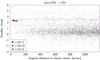 |
Fig. 1. Gaia DR2 parallaxes of all stars in the direction of the σ Ori cluster versus their Gaia DR2 distance to the cluster center taken at (RA, Dec) = (84.675, −2.6) deg from Simbad. The dashed and dotted horizontal lines indicate the mean and the limits of one standard deviation, respectively, of the parallaxes as determined by Caballero (2018) from cluster members. The positions of σ Ori C, D, and E in the diagram are indicated by the blue and red filled circles and the green filled diamond, respectively. |
The three bright stars σ Ori C, D, and E are highlighted in Fig. 1 with filled circles of different colors. They are close to the center of the cluster and have smaller parallaxes than the mean of the cluster. σ Ori E, in particular, at a Gaia DR2 angular distance of 80.4 arcsec on the sky from the cluster center has a parallax of 2.28 ± 0.10 mas, which gives a distance of  pc. This places it towards the furthest edge of the cluster (similarly to σ Ori C and D), as shown by the green dashed vertical line in Fig. 2. This comes in contrast to the distance estimate of 387.5 ± 1.3 pc for the triple σ Ori A and B system determined by Schaefer et al. (2016) from interferometric measurements (no Gaia DR2 parallax is available for σ Ori AB as it is too bright). The various astrometric quality checks are nevertheless good for σ Ori E: ten visibility periods are used in the astrometric calculation, the astrometric excess noise of 0.25 mas is not significant, and the parallax uncertainty is less than 5% (see below). The distance to σ Ori E derived from the Gaia DR2 parallaxes should therefore be reliable.
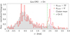 |
Fig. 2. Histograms of the Gaia DR2 parallaxes of all stars within a distance on the sky of 6 arcmin (open red histogram) and 20 arcmin (filled gray histogram) of the cluster center taken at the same position as in Fig. 1. The histograms are area-normalized. The vertical magenta dashed line locates the mean Gaia DR2 parallax of the cluster as determined by Caballero (2018). The vertical green dashed line locates the Gaia DR2 parallax of σ Ori E. |
The parallax uncertainties are shown in Fig. 3 versus parallaxes for all stars within a sky distance of 20 arcmin of the cluster center. The great majority of stars with parallaxes between 2 mas and 3 mas, i.e., potential cluster members, have a parallax uncertainty of better than 20%, and almost half of them, including σ Ori E, have parallax uncertainties of better than 5%.
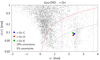 |
Fig. 3. Gaia DR2 parallax uncertainties versus parallax of all stars within a distance on the sky of 20 arcmin to the cluster center taken at the same position as in Fig. 1. The dashed and dotted vertical lines indicate the mean and limits of one standard deviation, respectively, of the parallaxes as determined by Caballero (2018) from cluster members. The red and gray solid lines indicate the parallax uncertainty limit at any given parallax below which the relative uncertainty is less than 20% and 5%, respectively. The positions of σ Ori C, D, and E in the diagram are indicated by the blue and red filled circles and the green filled diamond, respectively. |
An estimate of the systematic parallax uncertainties is more difficult to obtain, as it depends on many factors (see, Luri et al. 2018). If we take the systematic uncertainty of 0.029 mas derived by Luri et al. (2018) from the distribution of quasars, the corrected distance to σ Ori E would be 433 pc, which is within the uncertainties of the uncorrected distance.
With respect to the DR2, the early DR3 (EDR3) still allows a slight improvement of the parallax. This latter gives a parallax of 2.31 ± 0.06 mas, implying a distance of 433 ± 11 pc. This EDR3 distance is in good agreement with the distance of 439 pc obtained above from DR2.
In addition, new photometric data published in EDR3 from the Image Parameters Determination (IPD) module (Lindegren et al. 2021) confirm the absence of significant flux structures in the image window around σ Ori E. A first parameter, ipd_frac_multi_peak, indicates the fraction of valid transits for which another peak is observed in the image window around the source. For σ Ori E, this parameter is equal to zero, which means that only one peak is detected in the image window of σ Ori E for all transits used in the astrometric solution. A second parameter, ipd_gof_harmonic_amplitude, with a small value of 0.015 for σ Ori E, indicates that the goodness-of-fit of the flux distribution is independent of scan angle. Both these indicators point to the absence of significant structures in the flux distribution around σ Ori E such those resulting from the presence of a second source or specific patch patterns around the source, and thereby support the reliability of the distances derived from DR2 and EDR3 parallaxes.
2.2. Observed properties of σ Ori E
In Table 1, we have collected the data deduced from observations characterizing σ Ori E (HD 37479). The angular diameter, θ = 0.079 ± 0.002 mas, was obtained by Groote & Hunger (1982) using the formula θ = 2(Fearth/Ftheo.)1/2, where Fearth is the integrated flux received on Earth, and Ftheo. is a theoretical absolute flux determined using Kurucz’ model atmospheres.
Observational data for σ Ori E.
Using the distance determined by Gaia (DR2,  pc) and the angular diameter, one can determine the radius of σ Ori E (3.73 ± 0.26 R⊙). The effective temperature (22 500 ± 600 K) is deduced from the flux received on Earth and the angular diameter. This value is in agreement with the spectroscopic determination of the effective temperature by Hunger et al. (1989). We note that the recent determination by Oksala et al. (2012) using high-resolution spectropolarimetry finds an effective temperature of around 23 000 ± 3000 K2, which is also not fundamentally different from the one obtained by Groote & Hunger (1982). From the rotational period and the radius of the star, one can deduce the surface equatorial velocity (159 ± 11 km s−1). Using the radius and the effective temperature, one can determine the luminosity of σ Ori E quoted in Table 2. This luminosity is in agreement with the spectroscopically determined luminosity by Shultz et al. (2019b); see Table 1. Shultz et al. (2019b) also provides a value for the effective gravity, which is also shown in Table 1.
Properties of σ Ori E to be fitted by stellar models.
We do not consider the surface magnetic field or the surface abundances as constraints of the present models. As indicated in the previous section, the true morphology of the surface magnetic field is more complex than the one used here to model the wind magnetic braking. Therefore, the only quantity that we can hope to obtain is the value of an equivalent surface equatorial magnetic field in a pure aligned dipolar morphology that can fit both the surface rotation and the spin-down timescale. The fitting value provides an estimate of the field but this can differ from the observed one.
σ Ori E presents surface chemical inhomogeneities, which are likely produced by microscopic diffusion that might occur in atmosphere stabilized by a strong magnetic field (see e.g., Michaud 1970). In the entire class of Bp/Ap stars, these chemical inhomogeneities have been well documented for decades (Babcock 1947; Wolff 1968; Landstreet & Borra 1978). Recently, Panei et al. (2021) explored the question of chemical inhomogeneities at the surface of magnetic early B-stars. As these processes are not accounted for in the present models, we cannot use the observed surface abundances as constraints. On the other hand, we may see whether rotational mixing is expected to have occurred in σ Ori E. As we discuss below, the age we obtain is too short for the rotational mixing included in the present models to have a measurable effect.
3. Physics of the models
Stellar models are computed with GENEC, the Geneva stellar evolution code. The physical ingredients are the same as those of Ekström et al. (2012a) for what concerns any nonmagnetic effects. We use the Schwarzschild criterion for convection with a modest overshooting given by an extension of the radius of 0.1 Hp, where Hp is the pressure scale height estimated at the Schwarzschild boundary. Rotational mixing is accounted for according to the shellular theory by Zahn (1992). The diffusion coefficients and the physics of rotation are implemented as explained in Ekström et al. (2012a). The mass-loss rate via stellar winds is used according to de Jager et al. (1988). The present rotating models account for the various effects of a surface magnetic field on massive star evolution (Meynet et al. 2011; Petit et al. 2017; Georgy et al. 2017; Keszthelyi et al. 2019, 2020).
Similarly to previous GENEC implementations (Meynet et al. 2011; Georgy et al. 2017; Keszthelyi et al. 2019), we account for wind magnetic braking and mass-loss quenching. The wind magnetic braking is accounted for following the recipe given by ud-Doula et al. (2009). The present magnetic braking timescale of 1.3 Myr was found to be well inside the range of values expected from the theory of wind magnetic braking given in ud-Doula et al. (2009), thereby supporting the view that the observed braking might be due to that process.
The rate of loss of spin angular momentum  due to magnetic braking is expressed by
![Mathematical equation: $$ \begin{aligned} \dot{J}_{\rm mb}=\frac{2}{3}\dot{M}_{\rm wind}\Omega R^{2}[0.29+(\eta _{*}+0.25)^{1/4}]^{2}, \end{aligned} $$](/articles/aa/full_html/2022/01/aa41512-21/aa41512-21-eq9.gif) (1)
(1)
where Ṁwind is the mass-loss rate the star would have in the absence of the magnetic field (this is ṀB=0), Ω the surface angular velocity, R the stellar radius,  the equatorial magnetic confinement parameter (ud-Doula & Owocki 2002), with Beq the equatorial magnetic field which is equal to half the polar field in case of a dipolar magnetic field aligned with the rotational axis, and υ∞ is the final wind velocity (i.e., the wind velocity when there is no longer acceleration). The quantity R[0.29 + (η* + 0.25)1/4] is the Alfvén radius, RA. As magnetic braking modifies the angular velocity of the stellar surface, the Geneva code implements Eq. (1) as a boundary condition of the internal angular momentum transport equation at the stellar surface, and modifies the total angular momentum content of the star.
We have implemented the effect of mass-loss quenching by the surface magnetic field in the same way as Petit et al. (2017). We assume that the magnetic field is constant in time (see the discussion in Sect. 5). The escaping wind fraction fB (number inferior to 1) is taken as
 (2)
(2)
where rc is the radius of the farthest closed loop of the magnetic field and is computed as a function of the Alfvén radius and the confinement parameter (for details, see Keszthelyi et al. 2017; Petit et al. 2017; ud-Doula & Owocki 2002). We do not account for the factor  , where RK is the Kepler corotation radius defined by R/W2/3, with
  (see Eq. (22) in ud-Doula et al. 2009). The quantity W is the ratio of the surface rotation to the Keplerian critical velocity, which is the velocity at which, keeping the stellar radius constant, the centrifugal acceleration balances the gravity at the equator. Not accounting for this factor (as done here) leads to overestimation of the effect of the magnetic mass-loss quenching. However, we note that this does not impact the angular momentum loss rate because this latter depends on the mass-loss rate in the absence of any magnetic mass-loss quenching. The reason for this is that the mass retained in the magnetosphere slows down the star and its effect is accounted for in the formula for the angular momentum loss. Therefore, we suspect that the mass-loss quenching here actually has a rather modest effect by modifying the way the total mass of the star decreases. In any case, for the cases considered here, the total mass removed remains very modest. As a numerical example, a 9 M⊙ star has a mass-loss rate of between 10−9 and 10−10 M⊙ per year during the MS phase; thus, it loses a fraction of its total mass that is less than 0.3% during the 30 Myr duration of the MS phase. The magnetic mass-loss quenching will still reduce that quantity. Considering our 9 M⊙ star, a surface magnetic field of 5 kG, and an average surface rotation during the MS phase of 200 km s−1, we have that the Alfvén radius RA (about 30 times the stellar radius) is larger than the Keplerian radius RK (around 15 times the stellar radius), and we therefore have a centrifugal magnetosphere (Petit et al. 2013). In this case, rotation impacts the dynamics of the magnetosphere significantly (Townsend et al. 2005) and may lead to rotationally modulated variations of spectroscopic or photometric diagnostics (such as e.g., Balmer lines, UV, X-rays; see e.g., Petit et al. 2013). When the magnetic mass-loss quenching is accounted for in such a star, the mass lost during the MS phase is only a few percent of the mass lost without that effect and amounts to 0.01% of the total mass of the star. We note that considering the data for σ Ori E indicated in Table 1, assuming a mass of around 9 M⊙, one obtains that the Alfvén radius is around 50 stellar radii and the Kepler radius is around 30 stellar radii. For single-star models, we considered models of 8.0, 8.4, 8.7, and 9.1 M⊙ with metallicities of Z = 0.014 and 0.020, initial rotations equal to 250, 350, and 450 km s−1, and an equatorial surface magnetic field of 3, 5, and 7 kG.
4. Models for σ Ori E
Figures 4 and 5 present the evolution of the surface equatorial velocity and the stellar radius as a function of time, the braking timescale, and the evolutionary tracks in the HR diagram. The gray regions in each panel indicate the observed values of the different physical quantities. In Table 3, each model is specified by its initial mass, rotation, surface magnetic field (see Cols. 1 to 3), the age range where the model can fit the surface velocity, the stellar radius, and the braking timescale (see Cols. 3 and 4 for the models with a metallicity equal to 0.014, and Cols. 7, 8, and 9 for the metallicity equal to 0.020). Columns 6 and 10 indicate whether the position of the star in the HR diagram can be fitted (Y) or not (N). When “No Sol.” is indicated for the age ranges, this means more precisely that there is no solution in the age range between 0 and 10 Myr. We use red colors to emphasize age ranges that are not coincident with the one given by the requirement of fitting the surface velocity. Boldfaced age ranges highlight the domains of ages allowing a simultaneous fit of all the constraints indicated in Table 2.
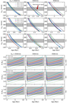 |
Fig. 4. Top panel: evolution of the surface equatorial velocity as a function of the age of the star for stellar models with various initial masses, metallicities, rotations, and surface magnetic fields. The shaded areas show the range of values for the surface equatorial velocity that can be deduced from the observed rotational period and from the stellar radius determined from the angular diameter and the Gaia distance. Bottom panel: evolution of the stellar radius as a function of the age of the star for stellar models with various initial masses, metallicities, rotations, and surface magnetic fields. The light shaded area shows the range of values for the stellar radii that can be deduced from the angular diameter and the Gaia distance. |
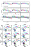 |
Fig. 5. Top panel: evolution of Ṗ/P, where P is the rotation period, for stellar models with various initial masses, metallicities, rotations, and surface magnetic fields. The light shaded area shows the range of values for the braking timescale as deduced by Townsend et al. (2010). Bottom panel: evolutionary tracks for stellar models with various initial masses, metallicities, rotations, and surface magnetic fields. Three black dashed lines indicate the isochrones with ages ranging from 10 to 30 Myr. The position of σ Ori E is indicated. |
Age range where the model fits the observed surface velocity, the observed radius, and the observed braking timescale, for each stellar model characterized by an initial mass, metallicity, rotation, and surface magnetic field.
4.1. Theoretical predictions
As shown in the left panel of Fig. 4, the surface equatorial velocity decreases as a function of time. A consequence of the strong surface rotation decrease is that very rapidly the star has a surface velocity that corresponds to a modest ratio of the critical velocity. The critical velocity is the surface equatorial velocity the star must have in order for the gravity at the equator to be balanced by the centrifugal force. As a numerical example, the critical surface velocity of stars3 with an initial mass of between 8 and 9.1 M⊙ and a radius compatible with the one indicated in Table 2 for σ Ori E is between 506 and 578 km s−1. Models that satisfy the observed constraints have surface velocities of between 150 and 170 km s−1. This represents a surface velocity equal to 26%−34% of the critical values. This ratio is too low for rotation to have any significant effect on the shape of the outer layers.
From the left panel of Fig. 4, we see that for a given initial rotation, the results do not show a great sensitivity to changes of the initial mass in the narrow mass interval between 8.0 and 9.1 M⊙. Increasing the surface magnetic field implies, as expected, a stronger braking. A given surface velocity is thus reached at an earlier time. The models at Z = 0.014 show a higher surface rotation at a given age than those at Z = 0.020. When the metallicity decreases, and stars are more compact and have weaker stellar winds, this decreases the loss of angular momentum at a given surface rotation rate and thus increases the braking timescale. Let us recall that a scaling of the wind with metallicity of the form  has been used here (as in the Geneva grids of stellar models Ekström et al. 2012a; Georgy et al. 2013).
The evolution of the stellar radius is shown in the upper panel of Fig. 4. Each curve shows two parts: an initial short phase where the radius decreases and a second long phase during which it increases. The first phase is due to the very efficient deceleration of the star by the magnetic wind braking effect. To understand this, it is important to remind ourselves that rotation deforms the star making it oblate; thus, the radius plotted in this panel is actually an average radius, defined as the radius of a spherical star that would have the same volume as the rotationally deformed star. As the polar radius is not significantly changed by rotation (see Fig. 2 in Ekström et al. 2008), and the equatorial radius increases when rotation increases, the volume of a star increases with rotation (Keszthelyi et al. 2020). When the star is decelerated, its volume decreases. This explains the first short phase of decreasing radius. At a given time, the braking timescale becomes long enough for the secular evolution of the star to become the main agent driving the evolution of the radius. As is well known, during the MS phase the radius increases and this is what we see in that second phase. The first phase lasts longer for the models starting with high initial rotation; it becomes shorter for the models with a high surface magnetic field. As is also well known, models at Z = 0.014 have smaller radii at a given age than models at Z = 0.020 (the difference in stellar radius is approximately 0.2 R⊙ between the two models with different metallicities).
The evolution of the braking timescale is shown in the left panel of Fig. 5. We can identify the two phases coming from the evolution of the radius described immediately above. In the first phase, the braking timescale increases rapidly due to the rapid deceleration of the star; it reaches a maximum then decreases. The decrease is mainly due to the fact that the mass-loss rate and the stellar radius increase during the evolution along the MS phase. Models with Z = 0.014 show longer braking timescales than those with Z = 0.020. At lower metallicities, the stars are more compact and the stellar winds are weaker, and therefore the angular momentum loss rate is weaker at a given surface velocity. We see that, for each model, a given braking timescale in a different fixed range for each model may occur at two different ages of the star: one at the very early time and one at a time when the age of the star is significantly above the braking timescale. This is due to the evolution described above.
In the lower panel of Fig. 5, we also see that lowering the metallicity shifts the tracks to hotter parts of the HR diagram. We see the consequences on the HR diagram of the short first phase during which the average radius decreases due to braking. This corresponds to the phase at the very beginning of each track, which is nearly horizontal. With luminosity remaining constant, the effective temperature increases. We note that the effective temperature defined here is also an average effective temperature. Indeed, according to von Zeipel theorem (von Zeipel 1924), the effective temperature varies as a function of the latitude when the star is rotating, with the poles being hotter than the equatorial regions. The effective temperature plotted in the figure is obtained as L/(4πR2), where R is the average radius.
4.2. Comparisons with σ Ori E
Using Figs. 4 and 5 (only the top panel), we can derive the range of ages of the models when they are inside the gray zone, that is, we can fit the corresponding property of σ Ori E deduced from the observations. The bottom panel of Fig. 5 does not directly allow us to deduce the age range (although some constant age lines are shown) but allows us to see whether the beginning of the tracks goes through the observed position of σ Ori E in the HR diagram.
The constraint coming from the surface velocity points towards a young star (see Cols. 4 and 8 of Table 3) with an age of between 0.4 and 2.5 Myr for all masses, initial rotations, metallicities, and surface magnetic fields considered here. Among the three other constraints, that on the magnetic braking timescale (see Cols. 6 and 10) is the most efficient in eliminating many models.
For the metallicity Z = 0.014, actually no models is found having a P/Ṗ compatible with the one observed in the age range given by the observed surface equatorial velocity (although sometimes the miss is due to a rather small incompatibility). The constrain of the radius at Z = 0.014 points to older ages than those needed to account for the surface velocity except in the case of the 8.7−9.1 M⊙ stellar models that are compatible with very young ages. The position in the HR diagram at Z = 0.014 favors masses around 8.0−8.7 M⊙.
For the metallicity Z = 0.020, only models with a surface equatorial magnetic field of around 7 kG provide a simultaneous fit to the constraints indicated in Table 2. Depending on the initial rotation, the age is either between 0.4 and 0.5 (250 km s−1), 0.6 and 0.7 (350 km s−1), or 0.75 and 0.9 (450 km s−1). As already mentioned above, for a given surface magnetic field, starting from a larger rotation allows the star to reach the observed surface velocity at a later time. At Z = 0.020, except for some models starting with 250 km s−1, the position in the HRD can always be fitted.
Consistent solutions are therefore easier to find at Z = 0.020 than at Z = 0.014. In Table 3, we have highlighted in boldface the range of ages where all the five constraints shown in Table 2 can be fitted. As mentioned above, only models at Z = 0.020 are found. More precisely, we cannot say that models with a metallicity of Z = 0.014 cannot reproduce the observed properties of σ Ori E, because we did not explore changes in the mass loss rate, convective core size, or different angular momentum transport for instance. It is beyond the scope of the present paper to explore all these possibilities, especially because, as discussed below, a metallicity of Z = 0.020 for σ Ori E is not unreasonable at the moment.
At first glance, the above results show that the models that best match the observed properties of σ Ori E have the following properties: an initial mass of between 8.4 and 9.1 M⊙, a metallicity of around Z = 0.020, an age of between 0.4 and 0.9 Myr, and finally magnetic braking similar to that due to a dipolar aligned magnetic field with an equatorial value of ∼7 kG. The high surface rotation and magnetic field of σ Ori E is possible because it is a very young single star.
We could have used the surface gravity of 4.2 ± 0.2 (see Table 1) according to Shultz et al. (2019b) as an additional constraint, but it would not lead to a better constraint in the model. Indeed, for all the four initial masses considered here of between 8.0 and 9.1 M⊙, the minimum and maximum radii allowed by the measured surface gravity define a region that overlaps and extends beyond the shaded region shown in the bottom panel of Fig. 4. Thus, any solution fitting the radius will fit the constraint of the surface gravity.
Figure 6 shows the evolution of the surface abundances of carbon and helium as a function of time. We see that the changes in helium abundance are very small with respect to those of carbon We note here that the abundance of carbon is normalized to that of hydrogen, while the abundance of helium is not. However, hydrogen does not change much and most of the variation shown for carbon is due to the change of carbon only. For carbon, models predict a decrease in abundance by a factor of two (0.3 dex) already after 8 Myr and for the models with an initial rotation larger than ∼350 km s−1. Helium needs much more time than carbon to show changes at the surface. This effect is due to the following phenomena: first let us recall that the diffusive velocity for a given element i scales as  , where Xi is the mass fraction of the element and ΔXi/Δr is the gradient of the abundance of this element. At the beginning there is no gradient, with zero age main sequence models being chemically homogeneous. In the absence of any mixing in the radiative zones, the gradients between the core and the envelope then evolve under the actions of both nuclear burning and convection. Helium increases at the center and carbon decreases due to the action of the CN cycle. The CN cycle is very rapid, much more rapid than the synthesis of helium. After one million years, in a star of 9 M⊙, the difference between the mass fraction of helium in the core and that in the envelope is 0.11 (in the core the mass fraction is 0.277 and in the envelope this is 0.266). For carbon, we obtain a mass fraction of 0.00003 in the core and 0.0023 in the envelope. A rough estimate of the ratio of the diffusive velocity over the same value of Δr will therefore be VHe/VC ≈ 0.011/0.271 × 0.0012/0.0023 ∼ 0.02. Thus, the diffusive velocity of helium is about only 2% of the diffusive velocity of carbon, and therefore the surface will show signs of the CN cycle before any significant change in helium abundance.
 |
Fig. 6. Evolution of the abundance ratios (given as ratios of the number density of the considered elements) at the surface as a function of time. Left panel: ratio of carbon to hydrogen. Right panel: ratio of helium to hydrogen. |
The value quoted by Oksala et al. (2012, 2015) (see Table 1 and Sect. 5.2) for the abundance of carbon (between −4.0 and −5.0 dex, see Table 1) cannot be reached at any time by the present models (more precisely, the most massive models at Z = 0.014 can reach a value of just below −4 dex after 8 Myr). It would be very interesting to have data for the nitrogen abundances to see whether this low carbon might be associated with an increase in nitrogen abundance. This would indicate the presence at the surface of material having been processed by the CN cycle, which very rapidly reaches equilibrium at the centre.
The observed helium surface abundances that are currently available (ϵHe between −1.1 dex and −0.6 dex) span a very large domain. σ Ori E presents an inhomogeneous surface composition due to processes such as microscopic diffusion in regions of the star where a strong magnetic field allows the atmosphere to be stabilized. Atomic diffusion as in Ap/Bp stars would mostly impact heavier elements, like Si and Fe-group, producing an anomaly with an overabundance of some elements and a deficit of others. We have not accounted for such processes in our models, and therefore we cannot make comparisons with the observed surface abundances. On the other hand, Fig. 6 shows that, for the very small ages obtained for σ Ori E using the present models (below 1 Myr), no changes are expected in the surface composition due to rotational mixing (as accounted for in the present models).
5. Discussion
5.1. The age of σ Ori E and the age of the σ Orionis open cluster
As the star σ Ori E belongs to the σ Ori cluster, it is logicial to ask the question of whether estimating the age of the cluster through isochrone fitting gives values that are compatible with the age deduced above for σ Ori E based on fitting the surface rotation, radius, breaking timescale, and position in the HR diagram. Let us reiterate that Sherry et al. (2008), Caballero (2007) obtained ages of between 2 and 3 Myr using these techniques, which is higher than what is inferred for σ Ori E in the present work. However, as is well known, age determination is a very model-dependent process.
Figure 7 presents the positions in the observational HR diagram of a sample of member candidates to the σ Ori cluster using Gaia EDR3 photometry and parallax. The member candidates are selected from an initial sample of sources within a circle of 600 arcsec radius around the center of the cluster, with the conditions 2 < ϖ[mas] < 3 on the parallax, 0.2 < PMRA[mas/yr] < 2.5 on the right-ascension proper motion, and −2.2 < PMDec[mas/yr] < 0.5 on the declination proper motion. These selection criteria favor purity of cluster membership rather than completeness. The candidates have been further restricted to those brighter than 19 mag in G and those with uncertainties in GBP − GRP of less than 0.1 mag. The GBP − GRP uncertainties and those of the absolute G magnitude are shown in Fig. 7. with horizontal and vertical bars, respectively, with the latter uncertainty including both photometric and parallax uncertainties. These uncertainties are smaller than the size of their data points in the figure for the great majority of the member candidates. It must be noted that past studies of this cluster came to the conclusion of very little reddening of its members (Béjar et al. 2001; Oliveira et al. 2002). We therefore did not apply any reddening correction.
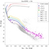 |
Fig. 7. Observed positions in the Gaia observational HR diagram of potential (see text) members of the σ Orionis cluster (magenta filled circles), with Gaia sources in the cluster field of view with parallaxes of better than 10% shown in small gray points in the background. The uncertainties on both photometry and parallax are shown for all cluster members, being smaller than the size of the points for the majority of them. Superposed are shown isochrones for a metallicity of Z = 0.014 from Haemmerlé et al. (2019) for different values of the logarithm of the age (in years). The positions of σ Ori C, D, and E are highlighted in the diagram as shown in the inset. |
Isochrones are also superposed in the same figure for different ages between 0.4 Myr (log(t) = 5.6) and 10 Myr (log(t) = 7.0) accounting for the pre-MS phase computed with accretion and no rotation by Haemmerlé et al. (2019) and a metallicity of Z = 0.0144. The isochrone passing through the observed position of σ Ori E is either an isochrone corresponding to a very young age with a log age of between 5.6 and 6.0 or an isochrone with a log age of greater than 7 (not shown here). However, a low age is likely the most reasonable solution in the case where most of the stars with a magnitude G of below 4.0 are indeed pre-MS stars. Thus, it appears that an age of 1 Myr for σ Ori E, as deduced above based on fitting the observed properties of σ Ori E, does not appear to be in contradiction with the age determined by isochrone fitting. We note however that this aspect would require more careful analysis and also a trial with similar isochrones but computed with a metallicity Z = 0.020.
5.2. The metallicity of σ Ori E
A solution is only obtained if the metallicity is around Z = 0.020. A value of 0.014 makes the finding of a solution more difficult if not impossible. As σ Ori E presents surface chemical inhomogeneities, direct determinations of its metallicity may be problematic. Oksala et al. (2015) in their Table 1 indicate values for ϵFe (=log(NFe/NH)) of between −5.7 and −4.0 for σ Ori E. For comparison, the solar value given by Scott et al. (2015) but in the same units as in Oksala et al. (2015) is −4.53. The large domain given by Oksala et al. (2015) does not allow a definitive conclusion as to whether σ Ori E is metal deficient or, on the contrary, slightly metal-rich compared to the Sun. Also, as already mentioned above, the Oksala abundances may not reflect the bulk iron abundance in the star or the diffusion processes that unevenly affect its surface composition. To obtain an idea of the true metallicity, it is better to rely on measurements of normal stars belonging to the same association. According to Cunha et al. (1998), the star HD 294297 belongs to the Ori OB 1b association where the σ Orionis cluster lies. These latter authors obtain an iron abundance (ϵFe) of −4.68 ± 0.14, which is below the solar abundance. If we assume that Z/Z⊙ = 10ϵFe − ϵFe⊙ (i.e., assuming a solar scaled distribution of the heavy elements), this would mean that Z is equal to 0.71 Z⊙ = 0.010 with Z⊙ = 0.014. If this metallicity is also the one corresponding to σ Ori E then our Z = 0.020 model is not an acceptable solution. In that case, either other parameters of the models should be changed to check whether a solution can be found at a metallicity lower than 0.020, or a more complex scenario involving multiple stars, as in for instance the merger of two stars, has to be invoked. However, it is currently difficult to discard the Z = 0.020 single-star evolution scenario on the basis of this metallicity measurement. If we look at Table 2 of Cunha et al. (1998), and compare the iron abundances for stars belonging to one association (here Ori OB 1c), they range from −4.8 (0.54 Z⊙ = 0.008 applying the same rule as above) up to −4.41 (1.32 Z⊙ = 0.018), which shows variations by a factor of 2.5. Moreover, Cunha et al. (1998) finds that the abundances of oxygen show still greater diversity than those of iron. These latter authors suggest that some regions where the observed stars have formed have been enriched by a nearby supernova. This would have an impact on the mass fraction of heavy elements Z. Therefore, it is still difficult to reach robust conclusions and more data need to be collected on the Ori OB 1b association.
In this work we have not considered different initial helium mass fractions at a given metallicity. Decreasing helium at a given metallicity shifts the position of the evolutionary tracks in the HR diagram to the red and may allow us to find a solution for a metallicity equal to Z = 0.014.
5.3. The magnitude of the surface magnetic field
The observed polar surface magnetic field of σ Ori E was obtained by Oksala et al. (2012, 2015). According to these authors, there is a dipolar component that is misaligned with respect to the rotation axis. The polar strength of this magnetic field is between 7.3 and 7.8 kG, with an obliquity of between 47° and 59° but there is also a smaller nonaxisymmetric quadrupole component with a strength of between 3 and 5 kG. A detailed modeling of the braking law resulting from the actual magnetic field topology would be an ideal solution. At the moment, based on the present simulations, we can only say that using an aligned dipolar configuration, we need a magnetic field polar strength of around 14 kG, thus larger than the observed one. This begs the question of whether a more realistic topology would lead to a model that needed a smaller polar field, more in line with the observed one. However, this is unlikely, because both the misalignment and the quadrupole components would be expected to decrease the braking efficiency overall compared to a pure aligned dipole. This question therefore remains open. We note that in this work we have not explored the possibility that the magnetic field flux may decay with time (discussions of possible underestimates of the braking efficiency and of the effect of magnetic flux decrease are presented by Keszthelyi et al. 2021 in their study of the B-type star tau Sco). However, the constraints given by the surface velocity and the isochrone fitting nevertheless favor a young age and thus a rather limited impact of this effect.
5.4. The timescale for diffusion
The star σ Ori E shows signs of the action of microscopic diffusion. We wonder whether the small age obtained gives enough time for such a process to impact the surface composition. According to Fig. 8.1 of Michaud et al. (2015), the diffusion timescales in a stable atmosphere of a 2.5 M⊙ star are between 103 and 104 years depending on the element considered (the diffusion timescale is the time for a given chemical element to diffuse over a pressure scale height). These timescales are much shorter than the age derived here for σ Ori E. However, these estimates are based on a non-magnetic atmosphere and are valid for stars with an effective temperature of lower than 16 000 K. Above these temperatures, stellar winds are expected to prevent any stratification due to diffusion. In the case of σ Ori E, the surface chemical inhomogeneities may be associated with regions stabilized by the strong magnetic field. Interestingly, the presence of a magnetic field does not significantly change the timescales indicated above (Georges Alecian, priv. comm. and see also Fig. 1 in Stift & Alecian 2016). Thus, from this discussion, we conclude that diffusion likely has enough time to operate, at least in some stabilized regions, on timescales of less than 1 Myr.
6. The σ Ori E analogs
In this section, we briefly discuss a few cases of σ Ori E analogs, that is, of B-type stars presenting both a high surface rotation and a strong surface magnetic field. The positions of these stars in the HR diagram are shown in Fig. 8. In Table 4, some properties of such stars are listed together with those of σ Ori E. From the mean positions of these stars in Fig. 8 (not accounting for the error bars), we can deduce the mass and radius of each star as would be given by the stellar models, and therefore also their critical velocity. From the υ sin i indicated, we then obtain the minimum ratios of the true equatorial velocity to the critical velocity. We obtain values of between about 25% (HD 23478) and 70% (HR 5907). According to Ekström et al. (2008), a 70% ratio means that the equatorial radius is about 20% larger than the polar one, implying some significant deformation.
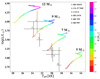 |
Fig. 8. Positions of σ Ori E and analogous stars in the HR diagram. The data for σ Ori E are those indicated in Table 2. For the other stars, the data have been taken as given in Table 1 of Shultz et al. (2020), except for the star CD –57°3509 taken from Przybilla et al. (2016). Main-Sequence rotating tracks from Ekström et al. (2012a) for the 5, 7, 9 and 12 M⊙ are indicated. |
Characteristics of some σ Ori E analogs ordered by decreasing υ sin i.
Fast-spinning stars with a strong surface magnetic field can be classified into two categories: those for which there is evidence that they are so young that fast rotation together with a strong surface magnetic field is not actually challenging single star models (like σ Ori E) and those for which evidence exists for a sufficiently high age or advanced evolutionary stage that present single star models cannot account for their properties. This second category requires either that the wind magnetic braking law does not apply or that an interaction with a companion (in the case of a merging event in the recent past) has spun up the star. Looking at Fig. 8, most of these stars have positions in the HRD compatible with a young age, except HD 345439 where the uncertainties do not allow firm conclusions to be drawn regarding its evolutionary status. In the discussion below, let us keep in mind that the age determinations are obtained from various different modeling assumptions, making this quantity highly uncertain.
HR 7355 (HD 182180) is a helium-strong chemically peculiar star with Balmer emission lines (Rivinius et al. 2008, 2013; Oksala et al. 2010). It shows He-strong absorption and polar field strength between 11 and 12 kG. Its rotation is exceptionally fast with a spin period of 0.52 days (Rivinius et al. 2008; Mikulášek et al. 2010), implying a surface velocity of υeq = 310 ± 5 km s−1 (Rivinius et al. 2013). Mikulášek et al. (2010) estimate the age to be between 15 and 25 Myr and a mass of 6.3 ± 0.3 M⊙ using isochrones from Marigo et al. (2008)5. Mikulášek et al. (2010) found a characteristic braking timescale of about 0.4 Myr, under the assumption that the star is a solid-body rotator. This short timescale would imply that the star is rapidly undergoing very efficient magnetic braking, suggesting a young age6. Thus this would be a challenging case for single star evolution. However, a study by Rivinius et al. (2013) showed that this case might not be so challenging after all if the gravity darkening effects are properly accounted for (see e.g., von Zeipel 1924; Espinosa Lara & Rieutord 2011), which are certainly important for such a fast rotating star (see Fig. 2 in Georgy et al. 2014). Rivinius et al. (2013) redetermined the properties of this star accounting for these effects and found a significantly lower mean effective temperature than previously found. From that lower effective temperature, they deduce weaker winds and thus a longer magnetic wind braking timescale. In contrast with previous works, these authors conclude that the age and rapid rotation are not inconsistent with the presence of a fossil magnetic field. This case illustrates the fact that at high rotation, one cannot neglect the effects of the deformation of the star.
According to Grunhut et al. (2012), HR 5907 (or HD 142184 or V1040 Sco) has a spin period of 0.51 days and an equatorial surface velocity of 340 km s−1 (Frémat et al. 2005); the star has an effective temperature of 17 000 ± 1000 K, a projected rotational velocity of 290 ± 10 km s−1, an equatorial radius of 3.1 ± 0.2 R⊙ a stellar mass of 5.5 ± 0.5 M⊙, and a surface dipole field strength of between ∼10.4 and 15.7 kG. (V = 5.4, B2.5V). It is located in the Upper Scorpius OB association at a distance of ∼145 pc7 (Hernández et al. 2005). Grunhut et al. (2012) also computed the spin-down timescale and found a value of about 8 Myr which is longer than the estimated age of HR 5907 by Hernández et al. (2005), but shorter than the age estimate of 10 Myr by Feiden (2016)8. Therefore, depending on the age estimate, this star may or may not be a challenging case for single star models.
Two stars HD 345439 and HD 23478 were discovered serendipitously in the course of the APOGEE (Apache Point Observatory Galactic Evolution Experiment) survey (Eikenberry et al. 2014). These latter authors detected the characteristic double-horned profile of emission lines in the Brackett series. This feature comes from material trapped in a magnetosphere rotating rigidly with the star (for a model of a rigidly rotating magnestosphere, RRM, see Townsend & Owocki 2005; Townsend et al. 2010). For HD 345439, these authors deduced υ sin i = 270 ± 20 km s−1 from the line profile of the He I absorption feature. They were not able to measure the magnetic field from their data, but the presence of a strong magnetic field is made evident through the presence of this RRM. Hubrig et al. (2015), using four subsequent low-resolution FORS 2 spectropolarimetric observations of that star, did not detect any magnetic field at a significance level of 3σ. However, this null result may be due to a rapidly varying magnetic field. The analysis of the four individual spectropolarimetric observations of that star by these latter authors is compatible with a variation of about 1 kG of the longitudinal magnetic field in a period of 88 min. The spectral type of HD 345439 indicates that it might be similar in mass to σ Ori E. It is difficult to say whether this star poses a challenge in the sense that little is known about its age.
Similarly to HD 345439, HD 23478 is a fast rotating star of the σ Ori E type that shows the presence of an RRM (for a detailed study see Sikora et al. 2015). However it is a “He-normal” B3IV star (Eikenberry et al. 2014). A υ sin i = 125 ± 20 km s−1 is obtained from the line profile of the He I absorption feature9. Its sky position and proper motion are compatible with it belonging to the IC 348 young open cluster (proper motions of stars in this cluster have been studied by Scholz et al. 1999). If it is indeed a member of that cluster, then the age of that star would be between 1.3 and 3 Myr according to Herbig (1998) and between 5 and 6 Myr according to Bell et al. (2013). Hubrig et al. (2015) performing low-resolution FORS 2 spectropolarimetric observations of that star discovered a rather strong longitudinal magnetic field of up to 1.3−1.5 kG (this is the magnetic field along the line of sight). This star might be an interesting candidate to study in a similar way to σ Ori E. It would be useful to have data on the braking timescale.
CPD –57°3509 (B2IV) is a member of the Galactic open cluster NGC 3293, and has an age of about 8 Myr (Baume et al. 2003). Przybilla et al. (2016) detected a surface averaged longitudinal magnetic field with a maximum amplitude of about 1 kG. They deduce this star has a bipolar magnetic field with a strength of greater than 3.3 kG (assuming a dipolar configuration). Also, they observe large and fast amplitude variations (within about 1 day) of the longitudinal magnetic field and interpret these as being the reflection of a very fast rotation (although the projected rotational velocity is small, around 35 km s−1). The star shows no sign of a RRM. Przybilla et al. (2016) obtain an effective temperature of 23750 ± 250 K and a log g of 4.05 ± 0.10, and using the Geneva track (Ekström et al. 2012b), they deduce a mass of 9.7 ± 0.3 M⊙, a radius of 5.0 ± 0.9 R⊙, a Log L/L⊙ = 3.85 ± 0.13, and an age of 13.8+2.4−3.3 Myr. The characteristics deduced from the models by Brott et al. (2011) are respectively 9.2 ± 0.4 M⊙, 4.4+0.7−0.5 R⊙, log L/L⊙ = 3.76 ± 0.12, and an age of 13.0+1.7−4.0 Myr. They provide some range for the equatorial velocity between about 70 and 250 km s−1. This star might also be an interesting case for checking the process of wind magnetic braking. An important additional piece of information would be to determine Ṗ. However, given the high inclination of the star, it seems unlikely that this will be achieved in the near future.
7. Conclusions and future perspectives
Here we revisit the case of σ Ori E, with the benefit of more accurate distance determinations provided by Gaia and a new series of computations that account for both the wind magnetic braking and magnetic mass-loss quenching.
We find that σ Ori E is a very young star (age of less than 1 Myr) as was obtained by Townsend et al. (2010). The mass of σ Ori E is between 8 and 9 M⊙ and its metallicity Z (mass fraction of heavy elements) is around 0.020. The braking law can well reproduce the observed deceleration in the frame of an aligned dipolar magnetic field topology. In light of these findings we find that the polar magnetic field needed is around 14 kG, which is two times larger than that observed. We are not able to resolve this discrepancy. However, we note that the true magnetic field topology is more complex than a simple dipolar one and that the present models did not account for any evolution of the surface magnetic field with time. We obtain that the initial rotation of the models fitting σ Ori E is not adequately constrained and could be anywhere in the range studied here. Because of its very young age, models predict no significant changes in the surface abundances due to rotational mixing for the main isotopes of the CNO elements or for helium. This young age remains compatible with an impact of the microscopic diffusion at least in zones stabilized by the surface magnetic field. In regions where low carbon abundance is obtained, it would be very interesting to have nitrogen abundance determinations. If an increase in nitrogen were found, this would support the view that some material processed by the CN cycle has been brought to the surface.
We see that knowledge of both surface velocity and P/Ṗ is highly constraining and allows the elimination of many models. Also, a change in metallicity, typically from 0.014 to 0.020, significantly changes the capacity of the models to provide a good fit. It would be interesting to observe nonmagnetic stars in the σ Ori E cluster and to check whether indeed the metallicity is closer to 0.020 rather than 0.014.
It would be interesting to compute models tailored to sigma Ori E with different angular momentum transport. For instance, if the stars rotate as solid bodies then the surface velocity can be maintained at a higher level with everything else kept equal. Indeed, solid body rotation implies that angular momentum is continuously transported from the core to the envelope10. This implies a higher surface velocity at any given age. A higher surface velocity in turn implies a stronger braking mechanism. Therefore, models need to be computed to study the net effect. In addition, chemical mixing is significantly changed and this has an impact on the evolutionary tracks, making it difficult to estimate the effects of assuming a solid body rotation rate. This question merits a separate, dedicated study.
New Prot of 91.9 ms per year is measured by Petit et al. (in prep.). This gives, considering a rotation period of 1.19 days, a value of the ratio equal to 1.12 Myr.
However, these authors have not modeled the spectrum in detail and did not attempt to precisely determine the effective temperature.
We assume a Roche model here where the critical velocity is given by  .
.
No such isochrones are currently available for a metallicity Z = 0.020. A value of Z = 0.020 would shift the isochrones slightly to the right in Fig. 7.
Oksala et al. (2010) obtained a gravity log g equal to 3.95 which would support a younger age for this star.
Mikulášek et al. (2010) indeed found possible evidence for a lengthening of the rotational period with Ṗ/P = 2.4(8) 10−6 yr−1 during the last 20 years, i.e., 108 ms per year.
The Gaia parallaxes confirm this distance for HR 5907, with a parallax of 7.08 ± 0.14 mas from DR2 (141 ± 3 pc), and 6.990 ± 0.074 mas from EDR3 (143.06 ± 0.14 pc).
More precisely, these authors give age estimates for the Upper Scorpius association to which HR 5907 belongs.
A previous work obtained a photometric period of 1.0499 days which is slightly faster than the 1.19 days rotation period of σ Ori E (Jerzykiewicz 1993).
Local conservation of the angular momentum produces a decrease in the angular velocity in the outer expanding layers and an increase in the contracting core, and therefore solid body rotation requires deceleration of the core and acceleration of the envelope.
Acknowledgments
The authors thanks the anonymous referee for her/his constructive report that has helped improving the paper. They thank Georges Alecian for providing information on the microscopic diffusion timescales. This work was sponsored by the Swiss National Science Foundation (project number 200020-172505), National Natural Science Foundation of China (grant Nos. 11863003 and 12173010), Science and technology plan projects of Guizhou province (Grant No. [2018]5781). GM, SE, PE and CG have received funding from the European Research Council (ERC) under the European Union’s Horizon 2020 research and innovation programme (grant agreement No 833925, project STAREX). GAW acknowledges support from the Discovery Grants program of the Natural Sciences and Engineering Research Council (NSERC) of Canada. This work has made use of data from the European Space Agency (ESA) mission Gaia (https://www.cosmos.esa.int/gaia), processed by the Gaia Data Processing and Analysis Consortium (DPAC, https://www.cosmos.esa.int/web/gaia/dpac/consortium). Funding for the DPAC has been provided by national institutions, in particular the institutions participating in the Gaia Multilateral Agreement.
References
- Babcock, H. W. 1947, ApJ, 105, 105 [NASA ADS] [CrossRef] [Google Scholar]
- Baume, G., Vázquez, R. A., Carraro, G., & Feinstein, A. 2003, A&A, 402, 549 [NASA ADS] [CrossRef] [EDP Sciences] [Google Scholar]
- Béjar, V. J. S., Martín, E. L., Zapatero Osorio, M. R., et al. 2001, ApJ, 556, 830 [CrossRef] [Google Scholar]
- Bell, C. P. M., Naylor, T., Mayne, N. J., Jeffries, R. D., & Littlefair, S. P. 2013, MNRAS, 434, 806 [NASA ADS] [CrossRef] [Google Scholar]
- Brott, I., de Mink, S. E., Cantiello, M., et al. 2011, A&A, 530, A115 [NASA ADS] [CrossRef] [EDP Sciences] [Google Scholar]
- Caballero, J. A. 2007, A&A, 466, 917 [NASA ADS] [CrossRef] [EDP Sciences] [Google Scholar]
- Caballero, J. A. 2017, Astron. Nachr., 338, 629 [NASA ADS] [CrossRef] [Google Scholar]
- Caballero, J. A. 2018, Res. Notes Am. Astron. Soc., 2, 25 [Google Scholar]
- Cunha, K., Smith, V. V., & Lambert, D. L. 1998, ApJ, 493, 195 [NASA ADS] [CrossRef] [Google Scholar]
- de Jager, C., Nieuwenhuijzen, H., & van der Hucht, K. A. 1988, A&AS, 72, 281 [NASA ADS] [Google Scholar]
- Eikenberry, S. S., Chojnowski, S. D., Wisniewski, J., et al. 2014, ApJ, 784, L30 [NASA ADS] [CrossRef] [Google Scholar]
- Ekström, S., Meynet, G., Maeder, A., & Barblan, F. 2008, A&A, 478, 467 [Google Scholar]
- Ekström, S., Georgy, C., Eggenberger, P., et al. 2012a, A&A, 537, A146 [Google Scholar]
- Ekström, S., Georgy, C., Granada, A., Wyttenbach, A., & Meynet, G. 2012b, ASP Conf. Ser., 453, 353 [Google Scholar]
- Espinosa Lara, F., & Rieutord, M. 2011, A&A, 533, A43 [NASA ADS] [CrossRef] [EDP Sciences] [Google Scholar]
- Feiden, G. A. 2016, A&A, 593, A99 [NASA ADS] [CrossRef] [EDP Sciences] [Google Scholar]
- Frémat, Y., Zorec, J., Hubert, A.-M., & Floquet, M. 2005, A&A, 440, 305 [NASA ADS] [CrossRef] [EDP Sciences] [Google Scholar]
- Gaia Collaboration (Brown, A. G. A., et al.) 2018, A&A, 616, A1 [NASA ADS] [CrossRef] [EDP Sciences] [Google Scholar]
- Georgy, C., Ekström, S., Eggenberger, P., et al. 2013, A&A, 558, A103 [NASA ADS] [CrossRef] [EDP Sciences] [Google Scholar]
- Georgy, C., Granada, A., Ekström, S., et al. 2014, A&A, 566, A21 [NASA ADS] [CrossRef] [EDP Sciences] [Google Scholar]
- Georgy, C., Meynet, G., Ekström, S., et al. 2017, A&A, 599, L5 [NASA ADS] [CrossRef] [EDP Sciences] [Google Scholar]
- Groote, D., & Hunger, K. 1982, A&A, 116, 64 [Google Scholar]
- Grunhut, J. H., Rivinius, T., Wade, G. A., et al. 2012, MNRAS, 419, 1610 [CrossRef] [Google Scholar]
- Haemmerlé, L., Eggenberger, P., Ekström, S., et al. 2019, A&A, 624, A137 [NASA ADS] [CrossRef] [EDP Sciences] [Google Scholar]
- Herbig, G. H. 1998, ApJ, 497, 736 [NASA ADS] [CrossRef] [Google Scholar]
- Hernández, J., Calvet, N., Hartmann, L., et al. 2005, AJ, 129, 856 [CrossRef] [Google Scholar]
- Hubrig, S., Schöller, M., Fossati, L., et al. 2015, A&A, 578, L3 [NASA ADS] [CrossRef] [EDP Sciences] [Google Scholar]
- Hunger, K., Heber, U., & Groote, D. 1989, A&A, 224, 57 [NASA ADS] [Google Scholar]
- Jerzykiewicz, M. 1993, A&AS, 97, 421 [NASA ADS] [Google Scholar]
- Keszthelyi, Z., Wade, G. A., & Petit, V. 2017, IAU Symp., 329, 250 [NASA ADS] [Google Scholar]
- Keszthelyi, Z., Meynet, G., Georgy, C., et al. 2019, MNRAS, 485, 5843 [NASA ADS] [CrossRef] [Google Scholar]
- Keszthelyi, Z., Meynet, G., Shultz, M. E., et al. 2020, MNRAS, 493, 518 [NASA ADS] [CrossRef] [Google Scholar]
- Keszthelyi, Z., Meynet, G., Martins, F., de Koter, A., & David-Uraz, A. 2021, MNRAS, 504, 2474 [NASA ADS] [CrossRef] [Google Scholar]
- Krtička, J., Mikulášek, Z., Prvák, M., et al. 2020, MNRAS, 493, 2140 [Google Scholar]
- Landstreet, J. D., & Borra, E. F. 1978, ApJ, 224, L5 [NASA ADS] [CrossRef] [Google Scholar]
- Lindegren, L., Klioner, S. A., Hernández, J., et al. 2021, A&A, 649, A2 [EDP Sciences] [Google Scholar]
- Luri, X., Brown, A. G. A., Sarro, L. M., et al. 2018, A&A, 616, A9 [NASA ADS] [CrossRef] [EDP Sciences] [Google Scholar]
- Marigo, P., Girardi, L., Bressan, A., et al. 2008, A&A, 482, 883 [NASA ADS] [CrossRef] [EDP Sciences] [Google Scholar]
- Meynet, G., Eggenberger, P., & Maeder, A. 2011, A&A, 525, L11 [NASA ADS] [CrossRef] [EDP Sciences] [Google Scholar]
- Michaud, G. 1970, ApJ, 160, 641 [Google Scholar]
- Michaud, G., Alecian, G., & Richer, J. 2015, Atomic Diffusion in Stars (Switzerland: Springer International Publishing) [Google Scholar]
- Mikulášek, Z., Krtička, J., Henry, G. W., et al. 2008, A&A, 485, 585 [NASA ADS] [CrossRef] [EDP Sciences] [Google Scholar]
- Mikulášek, Z., Krtička, J., Henry, G. W., et al. 2010, A&A, 511, L7 [NASA ADS] [CrossRef] [EDP Sciences] [Google Scholar]
- Mikulášek, Z., Krtička, J., Henry, G. W., et al. 2011, A&A, 534, L5 [NASA ADS] [CrossRef] [EDP Sciences] [Google Scholar]
- Oksala, M. E., Wade, G. A., Marcolino, W. L. F., et al. 2010, MNRAS, 405, L51 [NASA ADS] [CrossRef] [Google Scholar]
- Oksala, M. E., Wade, G. A., Townsend, R. H. D., et al. 2012, MNRAS, 419, 959 [NASA ADS] [CrossRef] [Google Scholar]
- Oksala, M. E., Kochukhov, O., Krtička, J., et al. 2015, MNRAS, 451, 2015 [Google Scholar]
- Oliveira, J. M., Jeffries, R. D., Kenyon, M. J., Thompson, S. A., & Naylor, T. 2002, A&A, 382, L22 [NASA ADS] [CrossRef] [EDP Sciences] [Google Scholar]
- Osmer, P. S., & Peterson, D. M. 1974, ApJ, 187, 117 [CrossRef] [Google Scholar]
- Panei, J. A., Vallverdú, R. E., & Cidale, L. S. 2021, A&A, 650, A92 [NASA ADS] [CrossRef] [EDP Sciences] [Google Scholar]
- Petit, V., Owocki, S. P., Wade, G. A., et al. 2013, MNRAS, 429, 398 [NASA ADS] [CrossRef] [Google Scholar]
- Petit, V., Keszthelyi, Z., MacInnis, R., et al. 2017, MNRAS, 466, 1052 [NASA ADS] [CrossRef] [Google Scholar]
- Przybilla, N., Fossati, L., Hubrig, S., et al. 2016, A&A, 587, A7 [NASA ADS] [CrossRef] [EDP Sciences] [Google Scholar]
- Reiners, A., Stahl, O., Wolf, B., Kaufer, A., & Rivinius, T. 2000, A&A, 363, 585 [NASA ADS] [Google Scholar]
- Rivinius, T., Tefl, S. Å., Townsend, R. H. D., & Baade, D. 2008, A&A, 482, 255 [NASA ADS] [CrossRef] [EDP Sciences] [Google Scholar]
- Rivinius, T., Townsend, R. H. D., Kochukhov, O., et al. 2013, MNRAS, 429, 177 [NASA ADS] [CrossRef] [Google Scholar]
- Schaefer, G. H., Hummel, C. A., Gies, D. R., et al. 2016, AJ, 152, 213 [NASA ADS] [CrossRef] [Google Scholar]
- Scholz, R.-D., Brunzendorf, J., Ivanov, G., et al. 1999, A&AS, 137, 305 [NASA ADS] [CrossRef] [EDP Sciences] [Google Scholar]
- Scott, P., Asplund, M., Grevesse, N., Bergemann, M., & Sauval, A. J. 2015, A&A, 573, A26 [NASA ADS] [CrossRef] [EDP Sciences] [Google Scholar]
- Sherry, W. H., Walter, F. M., Wolk, S. J., & Adams, N. R. 2008, AJ, 135, 1616 [NASA ADS] [CrossRef] [Google Scholar]
- Shultz, M., Rivinius, T., Das, B., Wade, G. A., & Chandra, P. 2019a, MNRAS, 486, 5558 [CrossRef] [Google Scholar]
- Shultz, M. E., Wade, G. A., Rivinius, T., et al. 2019b, MNRAS, 485, 1508 [NASA ADS] [CrossRef] [Google Scholar]
- Shultz, M. E., Owocki, S., Rivinius, T., et al. 2020, MNRAS, 499, 5379 [NASA ADS] [CrossRef] [Google Scholar]
- Sikora, J., Wade, G. A., Bohlender, D. A., et al. 2015, MNRAS, 451, 1928 [NASA ADS] [CrossRef] [Google Scholar]
- Stift, M. J., & Alecian, G. 2016, MNRAS, 457, 74 [NASA ADS] [CrossRef] [Google Scholar]
- Townsend, R. H. D., & Owocki, S. P. 2005, MNRAS, 357, 251 [NASA ADS] [CrossRef] [Google Scholar]
- Townsend, R. H. D., Owocki, S. P., & Groote, D. 2005, ApJ, 630, L81 [NASA ADS] [CrossRef] [Google Scholar]
- Townsend, R. H. D., Oksala, M. E., Cohen, D. H., Owocki, S. P., & ud-Doula, A. 2010, ApJ, 714, L318 [NASA ADS] [CrossRef] [Google Scholar]
- Townsend, R. H. D., Rivinius, T., Rowe, J. F., et al. 2013, ApJ, 769, 33 [NASA ADS] [CrossRef] [Google Scholar]
- ud-Doula, A., & Owocki, S. P. 2002, ApJ, 576, 413 [NASA ADS] [CrossRef] [Google Scholar]
- ud-Doula, A., Owocki, S. P., & Townsend, R. H. D. 2009, MNRAS, 392, 1022 [CrossRef] [Google Scholar]
- von Zeipel, H. 1924, MNRAS, 84, 665 [NASA ADS] [CrossRef] [Google Scholar]
- Wolff, S. C. 1968, PASP, 80, 281 [NASA ADS] [CrossRef] [Google Scholar]
- Zahn, J.-P. 1992, A&A, 265, 115 [NASA ADS] [Google Scholar]
All Tables
Age range where the model fits the observed surface velocity, the observed radius, and the observed braking timescale, for each stellar model characterized by an initial mass, metallicity, rotation, and surface magnetic field.
All Figures
|
Fig. 1. Gaia DR2 parallaxes of all stars in the direction of the σ Ori cluster versus their Gaia DR2 distance to the cluster center taken at (RA, Dec) = (84.675, −2.6) deg from Simbad. The dashed and dotted horizontal lines indicate the mean and the limits of one standard deviation, respectively, of the parallaxes as determined by Caballero (2018) from cluster members. The positions of σ Ori C, D, and E in the diagram are indicated by the blue and red filled circles and the green filled diamond, respectively. |
| In the text | |
|
Fig. 2. Histograms of the Gaia DR2 parallaxes of all stars within a distance on the sky of 6 arcmin (open red histogram) and 20 arcmin (filled gray histogram) of the cluster center taken at the same position as in Fig. 1. The histograms are area-normalized. The vertical magenta dashed line locates the mean Gaia DR2 parallax of the cluster as determined by Caballero (2018). The vertical green dashed line locates the Gaia DR2 parallax of σ Ori E. |
| In the text | |
|
Fig. 3. Gaia DR2 parallax uncertainties versus parallax of all stars within a distance on the sky of 20 arcmin to the cluster center taken at the same position as in Fig. 1. The dashed and dotted vertical lines indicate the mean and limits of one standard deviation, respectively, of the parallaxes as determined by Caballero (2018) from cluster members. The red and gray solid lines indicate the parallax uncertainty limit at any given parallax below which the relative uncertainty is less than 20% and 5%, respectively. The positions of σ Ori C, D, and E in the diagram are indicated by the blue and red filled circles and the green filled diamond, respectively. |
| In the text | |
|
Fig. 4. Top panel: evolution of the surface equatorial velocity as a function of the age of the star for stellar models with various initial masses, metallicities, rotations, and surface magnetic fields. The shaded areas show the range of values for the surface equatorial velocity that can be deduced from the observed rotational period and from the stellar radius determined from the angular diameter and the Gaia distance. Bottom panel: evolution of the stellar radius as a function of the age of the star for stellar models with various initial masses, metallicities, rotations, and surface magnetic fields. The light shaded area shows the range of values for the stellar radii that can be deduced from the angular diameter and the Gaia distance. |
| In the text | |
|
Fig. 5. Top panel: evolution of Ṗ/P, where P is the rotation period, for stellar models with various initial masses, metallicities, rotations, and surface magnetic fields. The light shaded area shows the range of values for the braking timescale as deduced by Townsend et al. (2010). Bottom panel: evolutionary tracks for stellar models with various initial masses, metallicities, rotations, and surface magnetic fields. Three black dashed lines indicate the isochrones with ages ranging from 10 to 30 Myr. The position of σ Ori E is indicated. |
| In the text | |
|
Fig. 6. Evolution of the abundance ratios (given as ratios of the number density of the considered elements) at the surface as a function of time. Left panel: ratio of carbon to hydrogen. Right panel: ratio of helium to hydrogen. |
| In the text | |
|
Fig. 7. Observed positions in the Gaia observational HR diagram of potential (see text) members of the σ Orionis cluster (magenta filled circles), with Gaia sources in the cluster field of view with parallaxes of better than 10% shown in small gray points in the background. The uncertainties on both photometry and parallax are shown for all cluster members, being smaller than the size of the points for the majority of them. Superposed are shown isochrones for a metallicity of Z = 0.014 from Haemmerlé et al. (2019) for different values of the logarithm of the age (in years). The positions of σ Ori C, D, and E are highlighted in the diagram as shown in the inset. |
| In the text | |
|
Fig. 8. Positions of σ Ori E and analogous stars in the HR diagram. The data for σ Ori E are those indicated in Table 2. For the other stars, the data have been taken as given in Table 1 of Shultz et al. (2020), except for the star CD –57°3509 taken from Przybilla et al. (2016). Main-Sequence rotating tracks from Ekström et al. (2012a) for the 5, 7, 9 and 12 M⊙ are indicated. |
| In the text | |
Current usage metrics show cumulative count of Article Views (full-text article views including HTML views, PDF and ePub downloads, according to the available data) and Abstracts Views on Vision4Press platform.
Data correspond to usage on the plateform after 2015. The current usage metrics is available 48-96 hours after online publication and is updated daily on week days.
Initial download of the metrics may take a while.