| Issue |
A&A
Volume 657, January 2022
|
|
|---|---|---|
| Article Number | A112 | |
| Number of page(s) | 9 | |
| Section | Astrophysical processes | |
| DOI | https://doi.org/10.1051/0004-6361/202140997 | |
| Published online | 20 January 2022 | |
Laboratory modelling of equatorial ‘tongue’ accretion channels in young stellar objects caused by the Rayleigh-Taylor instability
1
LULI – CNRS, CEA, UPMC Univ Paris 06: Sorbonne Université, Ecole Polytechnique, Institut Polytechnique de Paris, 91128 Palaiseau cedex, France
e-mail: This email address is being protected from spambots. You need JavaScript enabled to view it.
2
Sorbonne Université, Observatoire de Paris, PSL Research University, LERMA, CNRS UMR 8112, 75005 Paris, France
3
IAP, Russian Academy of Sciences, 603950 Nizhny Novgorod, Russia
4
INAF – Osservatorio Astronomico di Palermo, Piazza del Parlamento 1, 90134 Palermo, Italy
5
ELI-NP, ‘Horia Hulubei’ National Institute for Physics and Nuclear Engineering, 30 Reactorului Street, 077125 Bucharest-Magurele, Romania
6
Department of Astronomy, Cornell University, Ithaca, NY 14853, USA
Received:
5
April
2021
Accepted:
21
October
2021
Abstract
Context. The equatorial accretion scenario, caused by the development of the Rayleigh-Taylor (RT) instability at the disk edge, was suggested by accurate three-dimensional magnetohydrodynamic (MHD) modelling, but no observational or experimental confirmation of such phenomena has been evidenced yet.
Aims. We studied the propagation of a laterally extended laser-generated plasma stream across a magnetic field and investigated if this kind of structure can be scaled to the case of equatorial ‘tongue’ accretion channels in young stellar objects (YSOs); if so, this would support the possibility of equatorial accretion in young accreting stars.
Methods. We conducted a scaled laboratory experiment at the PEARL laser facility. The experiment consists in an optical laser pulse that is focused onto the surface of a Teflon target. The irradiation of the target leads to the expansion of a hot plasma stream into the vacuum, perpendicularly to an externally applied magnetic field. We used a Mach-Zehnder interferometer to diagnose the plasma stream propagation along two axes, to obtain the three-dimensional distribution of the plasma stream.
Results. The laboratory experiment shows the propagation of a laterally extended laser-generated plasma stream across a magnetic field. We demonstrate that: (i) such a stream is subject to the development of the RT instability, and (ii) the stream, decomposed into tongues, is able to efficiently propagate perpendicular to the magnetic field. Based on numerical simulations, we show that the origin of the development of the instability in the laboratory is similar to that observed in MHD models of equatorial tongue accretion in YSOs.
Conclusions. As we verify that the laboratory plasma scales favourably to accretion inflows of YSOs, our laboratory results support the argument in favour of the possibility of the RT-instability-caused equatorial tongue accretion scenario in the astrophysical case.
Key words: instabilities / magnetohydrodynamics (MHD) / accretion, accretion disks / stars: pre-main sequence
© K. Burdonov et al. 2022
 Open Access article, published by EDP Sciences, under the terms of the Creative Commons Attribution License (https://creativecommons.org/licenses/by/4.0), which permits unrestricted use, distribution, and reproduction in any medium, provided the original work is properly cited.
1. Introduction
The dynamics of matter accretion onto the surface of young stellar objects (YSOs) has been the subject of intense research in the past few decades. Considerable efforts have been made in the theoretical and numerical interpretation of astronomical observations; however, due to limitations of the state-of-art instrumentation, the exact dynamics and morphology of the processes taking place on the scales of stellar objects have not been resolved. Therefore, the development of detailed models that illustrate the full three-dimensional dynamics of accreting inflows of matter will remain essential for shedding light on the physics of accretion (e.g., Romanova et al. 2002, 2003, 2004; Romanova et al. 2008, 2012; Bessolaz et al. 2008; Zanni & Ferreira 2009, 2013; Orlando et al. 2011; Blinova et al. 2016; Colombo et al. 2019).
Intriguing numerical results, presented in Kulkarni & Romanova (2008), were obtained almost ten years ago. The developed three-dimensional magnetohydrodynamic (MHD) model of accretion dynamics at the boundary of the accretion disk and magnetosphere of the young star allowed two scenarios of matter accretion to be determined. In the first case, funnel flows follow the magnetic field lines and deposit matter at high latitudes, close to the polar regions, which is consistent with the modern understanding of the process (e.g., Romanova et al. 2003). In the second case, tall thin tongues of plasma, arising from the development of the Rayleigh-Taylor (RT) instability (Zhou 2017a,b), penetrate the stellar magnetosphere in the equatorial plane, impacting the YSOs with higher accretion rates, even at low latitudes. A more recent analysis has shown that higher accretion rates can also be connected to the condition where the gravitational force is larger than the centrifugal force at the inner disk, that is, the effective gravity should be negative (Blinova et al. 2016). Accretion then becomes more unstable in the case of increasing negative effective gravity.
In this work we investigate the possibility of an RT instability developing at the border of an accretion disk that may contribute to the triggering of mass accretion onto the protostar. To this end, we conducted a laboratory experiment, in which we explored the development of the RT instability of a laser-created plasma stream propagating in a vacuum across an externally applied magnetic field and examined the scalability of the laboratory plasma and of the process of matter accretion according to the tongue formation scenario. As will be discussed in this article, our experimental results strengthen the argument in favour of the likeliness of the scenario of RT-driven equatorial matter accretion, as proposed in Kulkarni & Romanova (2008).
We note that the configuration in which a plasma stream propagates across a magnetic field has long been experimentally investigated (see e.g., Sucov et al. 1967; Bruneteau et al. 1970; Plechaty et al. 2013; García-Rubio et al. 2016; Ivanov et al. 2017; Tang et al. 2018; Khiar et al. 2019; Leal et al. 2020; Filippov et al. 2021). The most recent studies Plechaty et al. (2013), García-Rubio et al. (2016), Ivanov et al. (2017), Tang et al. (2018), Khiar et al. (2019), and Leal et al. (2020), investigated the overall plasma dynamics in such a configuration and revealed that the plasma is able to extend along the magnetic field with a plasma slab-like global morphology, where the plasma is being compressed by the magnetic field into a thin layer in the plane that contains the magnetic field. The specificity of our work with respect to the abovementioned studies is that here the surface of the target affected by laser irradiation is very large. This allows us to launch the plasma across the magnetic field over a wide area, from which we observe the development of the RT instability that breaks the spatially wide expanding plasma into many individual ‘tongues’.
The paper is organised as follows. In Sect. 2 we present the laboratory setup and discuss the parameters of laboratory plasma. In Sect. 3 we demonstrate the scalability of the laboratory experiment to the ideal MHD model of the equatorial tongue accretion in YSOs. In Sect. 4 we discuss the origin of the RT instability, supported by numerical modelling, and in Sect. 5 we discuss the results and draw conclusions.
2. Laboratory experiment
2.1. Experimental setup
The experiment was performed at the PEARL laser facility (Lozhkarev et al. 2007; Soloviev et al. 2017; Perevalov et al. 2020). The setup is shown in Fig. 1. An optical laser pulse with energy around 3 J with a 1 ns full width at half maximum duration at the wavelength 527 nm was focused onto the surface of a Teflon (CF2) target. The laser energy was deposited as follows on the target: A focusing lens with a 1 m focal length was used to make the beam converge towards the target. However, prior to reaching the target, as shown in Fig. 1, a mask in the form of a slit with a 10 cm wide central gap selects part of the beam. The target was not positioned at the focus of the lens, but was placed 10e.g.cm before the focal plane. Thus, the beam irradiating the target surface was characterised by a 1 mm by 10 mm quasi-rectangular spot. The laser intensity in that spot was around 3 × 10¹⁰ W cm−2. The irradiation of the target by the laser induced the ablation of the surface target material and the expansion of a hot plasma stream into the vacuum, along z as the main expansion axis and perpendicular to the externally applied magnetic field of 1.35 × 10⁵ G. The magnetic field, oriented along the x axis, was created by a Helmholtz coil, which maintained a spatially (∼2 cm) and temporally (∼1 μs) constant field over the scales of the experiment (1 cm and 100 ns; Luchinin et al. 2020). A Mach-Zehnder-interferometer-based optical imaging scheme was used to diagnose the plasma stream propagation. For this, an optical probe low-energy short-pulse beam (100 mJ, 100 fs) was used to obtain snapshots of the plasma during its evolution.
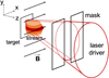 |
Fig. 1. Schematic view of the experimental setup. A laser beam with a rectangular shape (defined by a mask) propagates along the z axis and is focused on a target, the surface of which is positioned in the yz plane. An externally generated 1.35 × 10⁵ G magnetic field is applied to the whole space and is oriented along the x axis. |
This was done simultaneously along two axes, namely the x axis and y axis, providing two projections of the plasma density in order to obtain the three-dimensional distribution of the plasma stream. Such snapshots were captured at various times from 28 ns to 108 ns, after the start of the laser irradiation of the target (at t = 0), in 10 ns steps.
2.2. Laboratory plasma parameters
2.2.1. Laboratory plasma density analysis
The two-dimensional electron plasma density profiles in the yz plane (across the magnetic field) and xz plane (containing the magnetic field), at various instants in time, are shown in Fig. 2. It is clear from the yz-plane projection in Figs. 2a, c, e, and g that the development of an instability, namely the breaking down of the plasma flow into many sub-streams, takes place at early times and close to the surface of the target. In the xz-plane projection in Figs. 2b, d, f, and h, we do not observe any particular structure, meaning that in three dimensions the overall plasma structure is that (as depicted in Fig. 1) of a superposition of plasma tongues, that is, of layers of plasma extended into the xz plane (as the plasma can flow along the magnetic field lines) but compressed by the magnetic field in the yz plane. The plasma, starting initially as a single structure expanding from the target surface, clearly breaks down into several tongues. The view of the plasma in the xz-plane projection in Figs. 2b, d, f, and h being that of the stack of the sub-streams, we merely see an overall disk of plasma. At 28 ns (the earliest interferometry pattern registered in the experiment), we already observe developed and separated tongues, so the beginning of the instability that breaks the overall plasma into many tongues should take place before ∼10 ns, when the hot plasma stream is decelerated by the externally applied magnetic field. Once they are separated, the propagation of the tongues seems to take place with constant velocity (100 km s−1 for the mostly developed tongue). We note that the boundary separating the plasma stream and the tongues remains at a fixed location: It stays at a distance from the target of around 3–4 mm. The typical electron plasma density at that location is of the order of 1018 cm−3. We argue below that a likely explanation for the breakdown of the expanding plasma into the observed tongues is the RT instability.
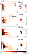 |
Fig. 2. Two-dimensional density profiles of the propagating plasma stream in the yz plane (a, c, e, and g) and the xz plane (b, d, f, and h) at 28 ns (a and b), 38 ns (c and d), 68 ns (e and f), 88 ns (g and h) after the laser irradiation of the target. The spatial scale, shown in (c), is the same for all the images. The colour bar is the same for all the images. The red ellipses on the left edge of the box in panels (g) and (h) represent the characteristic sizes in the yz and xz planes respectively, of the laser beam irradiating the target. |
Figure 3 shows the growth of the average spatial separation between the tongues. That average separation was calculated as follows: We took the length along the y axis over which the laser energy is deposited (see the red ellipse on the left edge of the box in Fig. 2g), and we divided it by the number of tongues that can be observed in the yz plane. It should be noted that here we counted the tongues at the distance of around 3 mm from the target surface.
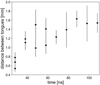 |
Fig. 3. Growth of the averaged distance between tongues, as inferred from the optical diagnostic of the expanding plasma, such as that shown in Fig. 2. Black points are the averaged distance values, and the black lines are the error bars. Each black dot on the graph corresponds to a unique shot. |
2.2.2. Laboratory plasma temperature analysis
The plasma temperature is likely to vary substantially along the main axis of propagation. Indeed, as analysed in detail in Khiar et al. (2019) and Filippov et al. (2021), the plasma that expands from the target, being fast and dense, has a higher (ram) pressure than that of the magnetic field (here, we estimated the initial ratio of the plasma ram pressure to the magnetic pressure to be ≈3). However, after a few millimetres, due to the decrease in the volumetric density of the plasma, the magnetic pressure can equilibrate with that of the plasma, inducing the formation of a shock at the plasma edge. The plasma is subsequently guided by the shock structure and channelled into the form of a tongue (i.e. the plasma is compressed by the magnetic field in the yz plane), while it can freely expand along the magnetic field in the xz plane. This is the case for plasma expanding from a small area, as in Khiar et al. (2019) and Filippov et al. (2021). On top of this, because the launching site is located in an extended area, we observe the breakup of the overall plasma into many sub-tongues. Therefore, we can distinguish two phases for the plasma during its propagation: (1) before the plasma is shocked and (2) thereafter. For phase (1) (i.e. within ≈1 mm of the target surface), we can estimate the plasma temperature along the propagation z axis using the Lagrangian one-dimensional hydrodynamic code ESTHER (Colombier et al. 2005; Bardy et al. 2020; Scius-Bertrand et al. 2020), which has been specially designed to simulate plasma formation in this low-laser-intensity and low-plasma-temperature regime.
The ESTHER code solves, according to a Lagrangian scheme, the fluid equations for the conservation of mass, momentum, and energy. The target material is described by the Bushman-Lomonosov-Fortov (BLF) multiphase equation of state, spanning a large range in density and temperature, from hot plasma to cold condensed matter. We used this code in these conditions since it specifically allows the transition from solid to plasma under the impact of a low intensity laser to be simulated (Colombier et al. 2005; Bardy et al. 2020; Scius-Bertrand et al. 2020), that is, it has an intensity of the order of 1010 W cm−2. Since the code cannot simulate the composite material (CF2) of the target, which has an average atomic mass of 17.3, the closest monoatomic target (in terms of mass) was used: pure carbon, with an atomic mass of 12. The background magnetic field is not treated in the simulation. ESTHER yields a plasma temperature of the order of ≈30 kK in the first millimetre of plasma propagation.
Later on, in phase (2), the magnetic field starts to impact the plasma stream propagation, as mentioned above. At the distance of around 2 mm from the target surface, where the plasma compression, and the formation of the thin tongues by the magnetic field becomes observable (see Fig. 2), the plasma temperature will increase, compared to the initial temperature, because of the shock induced in the plasma. We can estimate the ion temperature in shocked conditions as
![Mathematical equation: $$ \begin{aligned} T_{\rm i} = 6.25 \times 10^{14} \cdot \frac{3}{16 \times (Z+1)}m_{\rm i} [\mathrm{g}] \cdot { v}_{\rm i}^2[\mathrm{cm}], \end{aligned} $$](/articles/aa/full_html/2022/01/aa40997-21/aa40997-21-eq1.gif) (1)
(1)
where Z is the charge number, mi is the ion mass, and vi is the stream velocity (Zel’dovich & Raizer 2012). As can be seen in Table 1, the electron-ion equilibration time ( ; see Richardson 2019, p.34) is smaller than the timescales of the laboratory experiment. Therefore, Ti = Te. Obviously, Z depends on the plasma temperature and density, and this can be inferred from an atomic physics model such as FLYCHK (Chung et al. 2005). What we did was find the set of conditions (T, Z) that matched both Eq. (1) and FLYCHK for a plasma density of 1018 cm−3 (i.e. corresponding to the density in the tongue). This is verified for (T = 500 kK, Z = 6). Hence, we can state that the propagating plasma after the shock should have a temperature of around 500 kK. This value is used in the next section to estimate the scalability of the laboratory plasma to the YSO’s tongues of accretion.
3. Scalability
3.1. Accretion parameters
The tongues that are responsible for the equatorial accretion in YSOs have similar physical characteristics as the traditional funnel flows in which the matter streams along the magnetic field lines from the accretion disk to the stellar surface. The main difference is in their shape: The tongues are thin and elongated almost perpendicular to the equatorial plane, whilst the funnels are characterised by a loop-like shape.
The values of density, pressure, and velocity in the accretion stream vary from the accretion disk to the star surface (e.g., Romanova et al. 2002; Zanni & Ferreira 2009; Orlando et al. 2011). Typical ranges are presented below. Since the development of tongues requires high accretion rates, a realistic range of density to consider in YSOs is from 1013 cm−3 to 1014 cm−3. The velocity of the plasma inflow increases from the disk to the star, and, approaching the stellar surface, it can be of the order of a few hundred kilometres per second (e.g., Günther et al. 2006; Argiroffi et al. 2007). There are no constraints from observations for the temperature values; however, the expectation is that the plasma from the disk is relatively cold and that possible changes in temperature may occur along the tongue due to heating mechanisms. The realistic temperature range is from 1 kK to 10 kK. The magnetic field can be of the order of a few kilogauss at the stellar surface (e.g., Johns-Krull et al. 1999), and, considering that the large-scale field is almost dipolar, at the disk truncation radius it should be in the range from 10s G to 100s G.
We note that a series of other conditions needs to be met for the development of tongues. These are detailed in Kulkarni & Romanova (2008) and are as follows: small misalignment angles (< 30 deg) between the star’s rotation and magnetic axes; high accretion rates; a truncation radius of a few stellar radii (two to five); the stabilisation of instabilities via the tension of the azimuthal magnetic field (stellar magnetic field twisted by the inner disk plasma, which rotates faster than the star); and the stabilisation of instabilities via the radial shear of the angular velocity (to smear out the perturbations).
3.2. Scalability of laboratory plasma to YSOs
The scalability of the laboratory plasma stream to the accretion inflow of the YSOs is based on Ryutov’s ‘Euler similarity’ approach, which is described in detail in Ryutov et al. (1999, 2000), and Ryutov (2018).
Two systems are scaled to each other and evolve identically if they have two similar scaling quantities: the Euler number (Eu = V(ρ/p)1/2; here and below the formulas are all presented in cgs units) and the plasma beta (β = 8πp/B2), where V is the flow velocity, ρ is the mass density, p = kB(niTi + neTe) is the thermal pressure (kB is the Boltzmann constant, ni, e and Ti, e are the number densities and temperatures of the ions and electrons, respectively), and B is the magnetic field.
The Euler similarity can be applied in the case of the ideal MHD framework, where the dissipative processes, which might affect the fluid dynamics, can be neglected. The following parameters should be higher than 1 to meet the required conditions. This first is the Reynolds number, Re = LV/ν (the ratio of the inertial force to the viscous force), which is responsible for the viscous dissipation, where L is the characteristic spatial scale, V is the flow velocity, and
![Mathematical equation: $$ \begin{aligned} \nu [\mathrm{cm^2\,s^{-1}}] = 1.4 \times 10^9 \frac{T_{\rm i} [\mathrm{kK}]^{2.5}}{\Lambda \sqrt{A} Z^4 n_{\rm i}} \end{aligned} $$](/articles/aa/full_html/2022/01/aa40997-21/aa40997-21-eq6.gif) (2)
(2)
is the kinematic viscosity, where Λ is the Coulomb logarithm and A is the averaged atomic weight (Ryutov et al. 1999, p. 825). The second is the magnetic Reynolds number, ReM = LV/η (the ratio of the convection over Ohmic dissipation), which is responsible for the resistive diffusion. To derive ReM, we needed to evaluate the magnetic diffusivity,
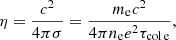 (3)
(3)
where σ is the electrical conductivity, me is the electron mass, e is the electron charge, and c2 = 1 (Ryutov et al. 2000, p. 467). Finally, the third is the Peclet number Pe = LV/χ (the ratio of heat convection to the heat conduction). This last parameter is the one responsible for the thermal conduction. It involves the thermal diffusivity (Ryutov et al. 1999, p. 824):
![Mathematical equation: $$ \begin{aligned} \chi [\mathrm{cm^2\, s^{-1}}] = 1.4 \times 10^{11} \frac{T_{\rm i} [\mathrm{kK}]^{2.5}}{\Lambda Z (Z+1) n_{\rm i}}. \end{aligned} $$](/articles/aa/full_html/2022/01/aa40997-21/aa40997-21-eq8.gif) (4)
(4)
We verified that all three parameters were indeed higher than one.
In Fig. 4a the phase-space of plausible YSO plasma beta values, depending on the star’s magnetic field strength, is shown. The grey area is bounded by the range of parameters of the YSO accretion inflows that were described in Sect. 3.1. The dotted vertical line corresponds to a laser-driven flow β that has an electron density of 5 × 1017 cm−3 and a temperature of 500 kK (i.e. relevant to the parameters of the individually propagating tongues). From this, we can infer the minimum and maximum magnetic field values of the YSOs in the range relevant to the laboratory plasma stream conditions, which are indicated by the horizontal dashed lines in Fig. 4a. Therefore, we can say that the laboratory stream is relevant to YSOs with a magnetic field strength in the range from ∼35 G to ∼350 G.
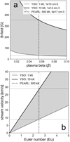 |
Fig. 4. (a) Correlation between the magnetic field and the plasma β (see text). The grey area corresponds to the range of YSO accretion flow parameters described in Sect. 3.1. The dotted vertical line marks the laser-driven flow β for electron plasma density 5 × 1017 cm−3 and temperature 500 kK (see Table 1), and the horizontal dashed lines correspond to the deduced minimum and maximum magnetic field values of the YSOs in the range of relevance to the laboratory plasma stream. (b) Correlation between the stream velocity and the Euler number. The dotted vertical line marks the laser-driven flow Eu, while the horizontal dashed lines correspond to the deduced minimum and maximum stream velocity values of the YSOs in the range relevant to the laboratory plasma stream. |
In Fig. 4b we show the phase-space of plausible YSO accretion stream velocities, depending on the stream Euler number (Eu). The dotted vertical line marks the laser-driven flow Eu (see Table 1 for details of the laser stream parameters). The horizontal dashed lines therefore correspond to the minimum and maximum stream velocity values of the YSOs in the range relevant to the laboratory plasma stream. From this, we inferred that the laboratory stream is relevant to YSO inflows that have velocities in the range from ∼10 km s−1 to ∼30 km s−1.
All these findings are summarised in Table 1, which details the parameters of the laboratory plasma stream as well as those of the YSO accretion inflow. For the latter, we considered two extreme cases: a colder, less dense accretion inflow and a hotter, denser one. The values of the density and temperature for each case correspond to the ranges described in Sect. 3.1. The characteristic laboratory scale considered here is 1 cm along the z axis (see Fig. 1) since this is the main plasma propagation axis against the magnetic field (i.e. relevant to the accretion phenomena of interest).
As can be seen from Table 1, the Reynolds number, the magnetic Reynolds number, and the Peclet number are all much higher than 1 for both the laboratory and the two considered cases of accretion inflows, thus satisfying the ideal MHD conditions. Moreover, the Euler number and plasma-β values are very well matched between the laboratory and the YSO flows, confirming the similarity of the evolution of the considered plasma flows. The scaling factors in space (amin, relevant to the colder and less dense accretion inflow case, and amax, relevant to the hotter and denser one), mass density (bmin and bmax), and velocity (cmin and cmax) between the YSOs and laboratory flows can be extracted. The spatial scaling parameters are
![Mathematical equation: $$ \begin{aligned} a_{\rm min} = \frac{r_{\rm min\,ast}}{r_{\rm lab}} = \frac{5\times 10^{6}\, \mathrm{[km]}}{1.0\, \mathrm{[cm]}} = 5 \times 10^{11}, \end{aligned} $$](/articles/aa/full_html/2022/01/aa40997-21/aa40997-21-eq9.gif) (5)
(5)
![Mathematical equation: $$ \begin{aligned} a_{\rm max} = \frac{r_{\rm max\,ast}}{r_{\rm lab}} = \frac{2\times 10^{6}\, \mathrm{[km]}}{1.0\, \mathrm{[cm]}} = 2 \times 10^{11}; \end{aligned} $$](/articles/aa/full_html/2022/01/aa40997-21/aa40997-21-eq10.gif) (6)
(6)
the mass density scaling parameters are
![Mathematical equation: $$ \begin{aligned} b_{\rm min} = \frac{\rho _{\rm min\,ast}}{\rho _{\rm lab}} = \frac{2.1 \times 10^{-11}\, [\mathrm{g \,cm}^{-3}]}{2.4 \times 10^{-6}\, [\mathrm{g \, cm}^{-3}]} = 8.8 \times 10^{-6}, \end{aligned} $$](/articles/aa/full_html/2022/01/aa40997-21/aa40997-21-eq11.gif) (7)
(7)
![Mathematical equation: $$ \begin{aligned} b_{\rm max} = \frac{\rho _{\rm max\,ast}}{\rho _{\rm lab}} = \frac{2.1 \times 10^{-10}\, [\mathrm{g \,cm}^{-3}]}{2.4 \times 10^{-6}\, [\mathrm{g \, cm}^{-3}]} = 8.8 \times 10^{-5}; \end{aligned} $$](/articles/aa/full_html/2022/01/aa40997-21/aa40997-21-eq12.gif) (8)
(8)
and the velocity scaling parameters are
![Mathematical equation: $$ \begin{aligned} c_{\min } = \frac{V_{\rm min\,ast}}{V_{\rm lab}} = \frac{10\, [\mathrm{km \,s^{-1}}]}{100 [\mathrm{km\, s^{-1}}]} = 0.1, \end{aligned} $$](/articles/aa/full_html/2022/01/aa40997-21/aa40997-21-eq13.gif) (9)
(9)
![Mathematical equation: $$ \begin{aligned} c_{\max } = \frac{V_{\rm max\,ast}}{V_{\rm lab}} = \frac{30\, [\mathrm{km\, s^{-1}}]}{100\, [\mathrm{km\, s^{-1}}]} = 0.3. \end{aligned} $$](/articles/aa/full_html/2022/01/aa40997-21/aa40997-21-eq14.gif) (10)
(10)
From all this, the following scalings on the base of these parameters can be retrieved. According to the temporal scaling, tast = (amin/max/cmin/max )tlab, 100 ns of the laser-driven flow is equivalent to around 5 × 10¹⁴ ns (∼6 days) of the astrophysical flow in the low-density, low-temperature case and to around 6.7 × 10¹³ ns (∼19 hours) in the case of high density and high temperature. According to the magnetic field scaling,  , 135 kG in the laser-driven flow case corresponds to ∼35 G in the lower and ∼350 G in the higher astrophysical case.
We note that here, as inferred from the first column of Table 1, the Hall parameter of the electrons in the tongue structures is larger than unity (i.e. He = ωc, eτe = le/RL, e = 8.3). Although it indicates that the electrons are magnetised in the tongue structures, the temperature (Te ∼ 500 kK) and its gradient in such structures are relatively low and heat transport in those regions is generally dominated by bulk plasma motions (i.e. Vflow ∼ 100 km s−1 and Pe ∼ 13). Similarly to what was discussed in Filippov et al. (2021), the electrons in the tongues being magnetised will not affect the magnetised RT instability, and the anisotropic thermal conduction does not play an important role here.
We also point out that a lower estimate of the magnetic Reynolds number, to quantify the relative importance of diffusion across the tongues, can be obtained by using the characteristic distance between the tongues, Ly ∼ 0.1 cm (see Fig. 3), and by assuming that the magnetic field is advected with the sound speed cs ∼ 50 km s−1. This gives ReM ∼ 3.5, indicating that magnetic diffusion is not the dominant effect.
3.3. Comparison with the Kulkarni-Romanova model
Initially, we observe that multiple small tongues form in the experiment. At later times, these tongues coalesce and form fewer, but more massive, tongues that propagate to larger distances across the field lines (see the sequence of panels a, c, e, and g in Fig. 2). Similar behaviour has been observed in the simulations of Kulkarni & Romanova (2008), who observed multiple small tongues at the beginning of their simulations, which coalesced to fewer, but larger, tongues. This is consistent with what can be expected from the RT instability in the linear approximation: Initially, small-scale wavelengths are expected to dominate, and their growth rate is faster than that of the large-scale modes (Chandrasekhar 1961). However, the propagation of smaller tongues is suppressed by the tension of the field lines, so they coalesce to larger, more massive tongues, which are able to propagate perpendicularly to the field lines (see Fig. 2).
Kulkarni & Romanova (2008) analysed such instabilities, taking different factors that led to the enhancement or suppression of the instability into account. They observed that the differential rotation in the inner disk is the main factor that can suppress the instability. They also observed that the boundary becomes more unstable when the accretion rate increases. A more detailed analysis by Blinova et al. (2016) has shown that the onset of the instability strongly depends on the effective gravity, geff = ggrav + gcentrifugal (i.e. it depends on the total force acting on the unit mass at the inner disk). If the gravitational force is larger than the centrifugal force by a certain value, then the accretion is always unstable (see Fig. 1 from Blinova et al. 2016). In the laboratory experiment, there is no centrifugal force, and the effects of gravity can be neglected. Instead, the pressure gradient force pushes matter perpendicularly to the field lines, thus playing the role of the gravitational force at the disk border in YSOs. This force decreases with distance, and unstable tongues become weaker with distance (see Fig. 2). In numerical simulations, the unstable tongues also weaken with distance because the dipole magnetic field strongly increases towards the star, faster than the effective gravity. Overall, the laboratory experiments confirm the results of the global three-dimensional MHD simulations of unstable accretion.
We should note that the RT instability has already been proposed to explain the mixing of plasma into the stellar magnetosphere in the case of spherical accretion (Arons & Lea 1976). Later, two-dimensional simulations (Wang & Robertson 1984) and three-dimensional simulations (Stone & Gardiner 2007) showed that the RT unstable filaments can penetrate deep into the region that has a plane-parallel homogeneous magnetic field that is perpendicular to gravity. Despite these results, it was somewhat amazing to see in three-dimensional MHD simulations that the RT unstable tongues can dominate accretion in magnetised stars that have a dipole magnetic field structure (Kulkarni & Romanova 2008). Our laboratory experiments confirm such a mode of RT unstable plasma flow at parameters that can be scaled to realistic parameters of YSOs (see Table 1).
4. Modelling of the RT instability under laboratory experiment conditions
4.1. Analytical estimates
We verified that the observed breakup of the plasma interface into many individual tongues is consistent with what we can expect from the growth of the RT instability. To do that, we needed to characterise the plasma condition in the first few nanoseconds after the laser impacts the target and verify if in these conditions the plasma interface can be unstable. As discussed in Sect. 2.2.2, this initial phase (before the development of the tongues) is simulated using the ESTHER code.
The plasma conditions retrieved from these simulations are shown in Fig. 5a. From them, we can estimate the wavelength of the fastest growing mode of the RT instability. Considering the effect of finite resistivity (which can damp the RT instability through the diffusion of the magnetic field) and the effect of viscosity (which can mitigate the instability growth through sheared velocities at fine scales), we localise the extrema of the growth rate function to be  . Here, η is the magnetic diffusivity, and the term k2η is the electrical resistive contribution to the RT instability dispersion relation; ν is the ion kinematic viscosity, and the term k2ν is the viscosity contribution (Green & Niblett 1960). We note that the relative importance of viscosity and resistivity as damping processes can be estimated from the ratio of these two terms, which is also equal to the ratio of the magnetic to the hydrodynamic Reynolds number (i.e. P = Rm/Re = ν/η). Using the Spitzer conductivity (Spitzer 1963) and the ion dynamic viscosity expression in the magnetised case given in Ryutov et al. 1999, we obtain
  , where ⟨A⟩ = 12 is the atomic number for carbon and ⟨Z(T)⟩ is interpolated from the FLYCHK database, considering a plasma density of 1018 cm−3 (Chung et al. 2005). We note that here in the low-temperature condition, which is valid within the first few nanoseconds after the laser irradiation, we used the Coulomb logarithm, Λ = 3 (Gericke et al. 2002). From this, we can conclude that P is always much smaller than unity within this temperature range (i.e. with the parameters mentioned above; e.g., for Tmax = 330 kK and Z = 4, P ∼ 5.0 × 10⁻⁵), indicating that the viscous term can be safely neglected. The wavelength of the fastest growing mode can be written as (Khiar et al. 2019)
![Mathematical equation: $$ \begin{aligned} \lambda _{\max }[\mathrm{m m}] \approx \pi {g}_{\mathrm{eff} }^{-1 / 3}\left(2.2 \times 10^{-3}\frac{\sqrt{\langle A\rangle } T^{5 / 2}}{\Lambda \langle Z\rangle ^{4} \rho }+3 \times 10^{9} \frac{\Lambda \langle Z\rangle }{T^{3 / 2}}\right)^{2 / 3} , \end{aligned} $$](/articles/aa/full_html/2022/01/aa40997-21/aa40997-21-eq18.gif) (11)
(11)
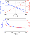 |
Fig. 5. (a) Plasma mass density (solid blue) and velocity (dash-dotted red) distribution along the z axis from the ESTHER simulation at 5 ns. The dashed blue line shows the best fit of the mass density lineout. (b) Temperature dependence of the fastest growing mode wavelength (solid blue) and the growth time (dashed red) for the RT instability, using the parameters from the ESTHER simulation at 5 ns around z = 350 μm for Eq. (11). |
where ρ = 0.03 kg m−3 is the local mass density (around z = 350 μm) and where T = Ti ∼ Te (which is justified since the thermal equilibration time is around 1 ns) is in units of kK. Furthermore, geff can be obtained by balancing the Lorentz force and the ram pressure force when the interface stagnates, namely  , where δsl ∼ 143 μm is the width of the interface fitted exponentially from the mass density distribution in Fig. 5a and v⊥ ∼ 80 km s−1 is the local velocity (also around z = 350 μm). Thus,
 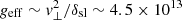 m s−2.
With the above parameters and equation, the temperature dependence of the fastest growing mode wavelength and growth time for the RT instability can be estimated. It is clear from Fig. 5b that over the temperature range of 40 − 330 kK the wavelength of the fastest growing mode is within 10 mm and flattens to a narrow band around 3 mm; this is in the same range as what can be retrieved from our experimental observations, as shown in Fig. 3. For these modes the growth time is around 3 ns, which explains the already fully developed tongue structures in the first experimental image obtained around 28 ns (see Fig. 2a). Here, the temperature range is lower than the temperature used in the scaling (i.e. 500 kK) because it is for the plasma-vacuum interface at an early time (i.e. within the first few nanoseconds after the laser irradiation), instead of the tongue structure after it has been shocked. By that time (after around tens of nanoseconds), the RT instability has indeed already fully developed.
4.2. Three-dimensional numerical modeling
To complement the analytical estimates of the growth of the RT instability in the conditions of the experiment detailed above, we performed numerical simulations. Our intent was not to do a one-to-one simulation of the experiment, which cannot be pursued with present-day computational capabilities and would thus be too demanding. Rather, we investigated the system dynamics of a reduced region of the target (x = 2.6 and y = 3.7 and z = 3.6 mm). We also restricted our investigation of the dynamics by neglecting collisions and using a pure hydrogen plasma.
To properly describe the ions-magnetic field interaction and to address the three-dimensionality of the problem, we chose the hybrid code Arbitrary Kinetic Algorithm (AKA; Sladkov 2020). In the numerical model, we kept the ion description at the particle level, while the electrons were described using the fluid dynamics from the ten-moments model. Those ten moments are density (n, equal to the total ion density by quasi-neutrality), bulk velocity (Ve), and the six-component electron pressure tensor (Pe). The electromagnetic fields are treated in the low-frequency (Darwin) approximation, neglecting the displacement current. The generalised Ohm’s law contains three terms: (i) Vi × B, where Vi is the ion bulk velocity covering the ideal MHD region; (ii) (J × B)/en, the Hall effect, where J is the total current density and is equal to the curl of B, which is important for the description of the ions decoupling from the magnetic field; and (iii) (∇·Pe)/en, the divergence of the electron pressure tensor, which represents the electron fluid contribution (Sladkov et al. 2021). In the model, the magnetic field and density are normalised to B0 = 6.75 ×10⁵ G and n0 = 2 × 1020 cm−3, respectively, and the normalisation of the other quantities follows from these ones. The density defines the ion inertial length, d0 ∼ 16 μm, which determines the length normalisation. The magnetic field defines the temporal normalisation since the time is normalised to the inverse of the ion gyrofrequency,  , which is ∼1 ns. Velocities are normalised to the Alfvén velocity, V0 (calculated using B0 and n0), which is 104 km s−1. In the simulation, the target density was initialised to 5n0 (i.e. 1021 cm−3), and the magnetic field (along the x axis) to 0.2B0 (i.e. 1.35 × 10⁵ G).
Continuous plasma production by the laser-target interaction is imitated by the ablation operator (Sladkov et al. 2020), which consists of both heat and particle creation operators. The heat operator linearly pumps the electron pressure into the near surface region of the target, creating a pressure gradient along the normal to the target surface; this generates an electric field and accelerates ions, thus initiating plasma expansion into the vacuum. The magnitude of the heat operator was adjusted to obtain the desired temperature ( = 1T0, which is 650 kK for the chosen parameters). The particle creation operator allows a constant target density to be sustained, mimicking the reservoir of a solid-density target. We used periodic boundaries for the long side of the plasma plume (see Fig. 6) and free boundary conditions in the two other directions. Figure 6 illustrates the temporal evolution of the plasma plume in the external magnetic field, as modelled by the simulations.
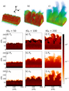 |
Fig. 6. Results of the three-dimensional hybrid simulation by the code AKA. Panels a–c show snapshots of plasma density at three time steps. Panels d–l display colour-coded plasma parameters for the two-dimensional central cut. Electron temperature, defined as one-third of the electron pressure tensor divided by density, is depicted in panels d–f. Panels g–i show the electron pressure, and panels j–l display the plasma density. The temporal and spatial normalisation factors are, respectively, |

The ablation operator is active for tΩ0 < 60, after which we observe the self-consistent cooling of the target in Figs. 6d–f. The expansion velocity initially achieves the maximum V0, 1.5V0 (∼150 km s−1), while the ram pressure exceeds the magnetic one (tΩ0 < 30). After deceleration, the velocity oscillates around 0.5V0 until the end of the simulations. At tΩ0 ∼ 50, we observe small-scale perturbations on the surface. Those perturbations are found in the compressed magnetic field layer (the thickness of which is about 10d0), where the plasma is of low density in Fig. 6j but where the electrons are hot in Fig. 6d. In that layer, the maximum temperature is a few times the initial focal spot temperature. At tΩ0 ∼ 100, the interior plasmas start to break through the hot layer. At tΩ0 ∼ 200, we observe the formation of clearly separated tongues, stretched from the core plasmas, which remain at an almost constant height of z ∼ 75d0 (see Fig. 6). The maximum width the two greatest tongues achieve is y ∼ 50d0 and their maximum height is twice the core plasma height, which is consistent with the experimental findings. The temperature of the tongues at later times is distributed uniformly in the core and is of the order of 0.1T0 (∼65 kK).
To estimate geff, we considered the y component of the Hall electric field (JzBx/n), which is responsible for the upward plasma drift in the crossed electromagnetic fields (Plechaty et al. 2013). Its magnitude at the front after breaking through the compressed layer is around 1. Once the layer is broken, the magnetic field magnitude drops from approximately B0 down to 0.25B0 at the top of the tongue, the characteristic current magnitude is ∼0.1J0, and the surface density is 2.5 × 10⁻²n0. For the chosen normalisation, geff ∼ 1.6 × 10¹³ m s−2, which is the same order of magnitude as the value derived above (see Sect. 4) based on the one-dimensional simulation of the early plasma expansion. The width of the tongues is 0.8 mm, which is also in good agreement with the value derived from our experiments.
While we do not take the plasma collisionality into account here, we should distinguish between two regions while discussing the effect of collisions: the interior of the plume and the shocked layer. In the interior, the diamagnetic plasma effect expels the external magnetic field, and the main source for the magnetic field is the electron pressure tensor fluctuations. Hence, ions are basically demagnetised inside the cavity. Regarding the shocked layer, which is accompanied by a compressed magnetic field, strong magnetisation of the ions is observed. In the shocked region, collisions are also less important due to a lower plasma density and a higher temperature. Hence, collisions are important close to the dense plasma generated by the laser and decrease approaching the shocked layer. In the shocked region, the Hall effect is significant because of the strong current and low density, and it is seen in the simulations to be the main contributor to the growth of the tongues.
5. Summary and conclusion
We conducted laboratory experiments at the PEARL laser facility that describe a laterally extended, hot laser-generated plasma stream expanding into a vacuum perpendicularly to an ambient magnetic field. During the evolution of the stream, we observed its breakup into many individual tongues. The development of these tongues seems to be consistent with what can be expected from the development of the RT instability in such plasma, based on analytical estimates and three-dimensional numerical modelling. We verified the good scalability of the laboratory plasma flows to the equatorial tongue accretion channels in YSOs, a scenario that was numerically investigated in Kulkarni & Romanova (2008). Overall, our investigation thus strengthens the argument supporting the tongue equatorial accretion scenario as a viable way of increasing the accretion rates in YSOs.
With these results, we hope to improve our understanding of the role played by the magnetic field in regulating the accretion of mass onto protostars and of the geometry of the accretion pattern. In fact, although the general picture of the accretion process in YSOs is clear, several aspects are still poorly constrained, including the geometry of the accretion structures. According to the largely accepted magnetospheric accretion paradigm, the stellar magnetic field disrupts the inner portion of the disk and channels the disk material in its flux tubes, guiding it in its fall towards the protostar (e.g., Koenigl 1991; Calvet & Hartmann 1992; Hartmann et al. 1994). At the end of its journey, the material impacts the stellar surface, with velocities of up to 300 − 500 km s−1, producing hot spots on the stellar surface due to shocks that convert the kinetic energy of the accreting material into thermal energy. Depending on the density and velocity of the accretion streams, the hot spots can be characterised by temperatures of a few million degrees and densities higher than 1011 cm−3 (e.g., Sacco et al. 2010).
Usually, the magnetic flux tubes that guide the disk material towards the star are assumed to form loop-like streams. In the case where a dipole component also dominates in the proximity of the star, the streams are expected to impact the stellar surface at high latitudes, thus producing the hot spots close to the polar regions (e.g., Romanova et al. 2003). However, in some cases, this prediction contrasts with the evidence that hot spots may also exist at low latitudes. This is, for instance, the case of the Classical T-Tauri star (CTTS) TW Hydrae, the observations of which clearly suggest that the dominant accretion spots are located at low latitudes (Argiroffi et al. 2017). This evidence can be explained as being due to complex configurations of the stellar magnetic field, as suggested by surface magnetograms of CTTSs (e.g., Gregory et al. 2008; Donati & Landstreet 2009). Our study suggests that equatorial tongue accretion channels (e.g., Kulkarni & Romanova 2008) can also be at work in CTTSs and, therefore, can provide an alternative explanation for the existence of low-latitude hot spots.
Acknowledgments
The authors would like to thank the team of the PEARL facility for their expert support. This work was supported by funding from the European Research Council (ERC) under the European Unions Horizon 2020 research and innovation program (Grant Agreement No. 787539). The research leading to these results is supported by Extreme Light Infrastructure Nuclear Physics (ELI-NP) Phase II, a project co-financed by the Romanian Government and European Union through the European Regional Development Fund, and by the project ELI-RO-2020-23 funded by IFA (Romania). The experiments at the PEARL facility (IAP RAS) were supported by the Russian Science Foundation (RSF) in the frame of project No. 20-12-00395. This work was granted access to the HPC resources of MesoPSL financed by the Region Ile de France and the project EquipMeso (reference ANR-10-EQPX29-01) of the programme Investissements d’Avenir supervised by the Agence Nationale pour la Recherche. R.B. acknowledges support from the project PRIN-INAF 2019 “Spectroscopically Tracing the Disk Dispersal Evolution”. M.M.R. acknowledges the NSF grant AST-20009820. The simulations were partially performed on resources provided by the Joint Supercomputer Center of the Russian Academy of Sciences.
References
- Argiroffi, C., Maggio, A., & Peres, G. 2007, A&A, 465, L5 [NASA ADS] [CrossRef] [EDP Sciences] [Google Scholar]
- Argiroffi, C., Drake, J. J., Bonito, R., et al. 2017, A&A, 607, A14 [NASA ADS] [CrossRef] [EDP Sciences] [Google Scholar]
- Arons, J., & Lea, S. M. 1976, ApJ, 207, 914 [Google Scholar]
- Bardy, S., Aubert, B., Bergara, T., et al. 2020, Opt. Laser Technol., 124, 105983 [NASA ADS] [CrossRef] [Google Scholar]
- Bessolaz, N., Zanni, C., Ferreira, J., Keppens, R., & Bouvier, J. 2008, A&A, 478, 155 [NASA ADS] [CrossRef] [EDP Sciences] [Google Scholar]
- Blinova, A. A., Romanova, M. M., & Lovelace, R. V. E. 2016, MNRAS, 459, 2354 [Google Scholar]
- Bruneteau, J., Fabre, E., Lamain, H., & Vasseur, P. 1970, Phys. Fluids, 13, 1795 [Google Scholar]
- Calvet, N., & Hartmann, L. 1992, ApJ, 386, 239 [CrossRef] [Google Scholar]
- Chandrasekhar, S. 1961, Hydrodynamic and Hydromagnetic Stability, International series of monographs on physics (Clarendon Press) [Google Scholar]
- Chung, H.-K., Chen, M., Morgan, W., Ralchenko, Y., & Lee, R. 2005, High Energy Density Phys., 1, 3 [NASA ADS] [CrossRef] [Google Scholar]
- Colombier, J. P., Combis, P., Bonneau, F., Le Harzic, R., & Audouard, E. 2005, Phys. Rev. B, 71, 165406 [Google Scholar]
- Colombo, S., Orlando, S., Peres, G., et al. 2019, A&A, 624, A50 [NASA ADS] [CrossRef] [EDP Sciences] [Google Scholar]
- Donati, J. F., & Landstreet, J. D. 2009, ARA&A, 47, 333 [Google Scholar]
- Filippov, E. D., Makarov, S. S., Burdonov, K. F., et al. 2021, Sci. Rep., 11, 8180 [NASA ADS] [CrossRef] [Google Scholar]
- García-Rubio, F., Ruocco, A., & Sanz, J. 2016, Phys. Plasmas, 23, 012103 [CrossRef] [Google Scholar]
- Gericke, D., Murillo, M., & Schlanges, M. 2002, Phys. Rev. E, 65, 036418 [NASA ADS] [CrossRef] [Google Scholar]
- Green, T., & Niblett, G. 1960, Nucl. Fusion, 1, 42 [CrossRef] [Google Scholar]
- Gregory, S. G., Matt, S. P., Donati, J. F., & Jardine, M. 2008, MNRAS, 389, 1839 [Google Scholar]
- Günther, H. M., Liefke, C., Schmitt, J. H. M. M., Robrade, J., & Ness, J. U. 2006, A&A, 459, L29 [NASA ADS] [CrossRef] [EDP Sciences] [Google Scholar]
- Hartmann, L., Hewett, R., & Calvet, N. 1994, ApJ, 426, 669 [Google Scholar]
- Ivanov, V. V., Maximov, A. V., Betti, R., et al. 2017, Plasma Phys. Control. Fusion, 59, 085008 [CrossRef] [Google Scholar]
- Johns-Krull, C. M., Valenti, J. A., Hatzes, A. P., & Kanaan, A. 1999, ApJ, 510, L41 [CrossRef] [Google Scholar]
- Khiar, B., Revet, G., Ciardi, A., et al. 2019, Phys. Rev. Lett., 123, 205001 [Google Scholar]
- Koenigl, A. 1991, ApJ, 370, L39 [Google Scholar]
- Kulkarni, A. K., & Romanova, M. M. 2008, MNRAS, 386, 673 [Google Scholar]
- Leal, L. S., Maximov, A. V., Betti, R., Sefkow, A. B., & Ivanov, V. V. 2020, Phys. Plasmas, 27, 022116 [NASA ADS] [CrossRef] [Google Scholar]
- Lozhkarev, V. V., Freidman, G. I., Ginzburg, V. N., et al. 2007, Laser Phys. Lett., 4, 421 [Google Scholar]
- Luchinin, A. G., Malyshev, V. A., Kopelovich, E. A., et al. 2020, Pulsed magnetic field generation system for laser-plasma research [Google Scholar]
- Orlando, S., Reale, F., Peres, G., & Mignone, A. 2011, MNRAS, 415, 3380 [Google Scholar]
- Perevalov, S. E., Burdonov, K. F., Kotov, A. V., et al. 2020, Plasma Phys. Controlled Fusion, 62, 094004 [NASA ADS] [CrossRef] [Google Scholar]
- Plechaty, C., Presura, R., & Esaulov, A. A. 2013, Phys. Rev. Lett., 111, 185002 [Google Scholar]
- Richardson, A. 2019, NRL Plasma Formulary (Washington, DC: Naval Research Laboratory) [Google Scholar]
- Romanova, M. M., Ustyugova, G. V., Koldoba, A. V., & Lovelace, R. V. E. 2002, ApJ, 578, 420 [Google Scholar]
- Romanova, M. M., Ustyugova, G. V., Koldoba, A. V., Wick, J. V., & Lovelace, R. V. E. 2003, ApJ, 595, 1009 [Google Scholar]
- Romanova, M. M., Ustyugova, G. V., Koldoba, A. V., & Lovelace, R. V. E. 2004, ApJ, 610, 920 [Google Scholar]
- Romanova, M. M., Kulkarni, A. K., & Lovelace, R. V. E. 2008, ApJ, 673, L171 [Google Scholar]
- Romanova, M. M., Ustyugova, G. V., Koldoba, A. V., & Lovelace, R. V. E. 2012, MNRAS, 421, 63 [NASA ADS] [Google Scholar]
- Ryutov, D. D. 2018, Phys. Plasmas, 25, 100501 [Google Scholar]
- Ryutov, D., Drake, R. P., Kane, J., et al. 1999, ApJ, 518, 821 [Google Scholar]
- Ryutov, D. D., Drake, R. P., & Remington, B. A. 2000, ApJS, 127, 465 [Google Scholar]
- Sacco, G. G., Orlando, S., Argiroffi, C., et al. 2010, A&A, 522, A55 [NASA ADS] [CrossRef] [EDP Sciences] [Google Scholar]
- Scius-Bertrand, M., Videau, L., Rondepierre, A., et al. 2020, J. Phys. D: Appl. Phys., 54, 055204 [Google Scholar]
- Sladkov, A. 2020, AKA code, https://github.com/dusse/AKA52 [Google Scholar]
- Sladkov, A., Smets, R., & Korzhimanov, A. 2020, J. Phys.: Conf. Ser., 1640, 012011 [NASA ADS] [CrossRef] [Google Scholar]
- Sladkov, A., Smets, R., Aunai, N., & Korzhimanov, A. 2021, Phys. Plasmas, 28, 072108 [NASA ADS] [CrossRef] [Google Scholar]
- Soloviev, A., Burdonov, K., Chen, S. N., et al. 2017, Sci. Rep., 7, 12144 [Google Scholar]
- Spitzer, L., Jr 1963, Am. J. Phys., 31, 890 [NASA ADS] [CrossRef] [Google Scholar]
- Stone, J. M., & Gardiner, T. 2007, ApJ, 671, 1726 [NASA ADS] [CrossRef] [Google Scholar]
- Sucov, E. W., Pack, J. L., Phelps, A. V., & Engelhardt, A. G. 1967, Phys. Fluids, 10, 2035 [Google Scholar]
- Tang, H., Hu, G., Liang, Y., et al. 2018, Plasma Phys. Controlled Fusion, 60, 055005 [NASA ADS] [CrossRef] [Google Scholar]
- Wang, Y. M., & Robertson, J. A. 1984, A&A, 139, 93 [NASA ADS] [Google Scholar]
- Zanni, C., & Ferreira, J. 2009, A&A, 508, 1117 [NASA ADS] [CrossRef] [EDP Sciences] [Google Scholar]
- Zanni, C., & Ferreira, J. 2013, A&A, 550, A99 [NASA ADS] [CrossRef] [EDP Sciences] [Google Scholar]
- Zel’dovich, Y., & Raizer, Y. 2012, Physics of Shock Waves and High-Temperature Hydrodynamic Phenomena, Dover Books on Physics (Dover Publications) [Google Scholar]
- Zhou, Y. 2017a, Phys. Rep., 720, 1 [Google Scholar]
- Zhou, Y. 2017b, Phys. Rep., 723, 1 [Google Scholar]
All Tables
All Figures
|
Fig. 1. Schematic view of the experimental setup. A laser beam with a rectangular shape (defined by a mask) propagates along the z axis and is focused on a target, the surface of which is positioned in the yz plane. An externally generated 1.35 × 10⁵ G magnetic field is applied to the whole space and is oriented along the x axis. |
| In the text | |
|
Fig. 2. Two-dimensional density profiles of the propagating plasma stream in the yz plane (a, c, e, and g) and the xz plane (b, d, f, and h) at 28 ns (a and b), 38 ns (c and d), 68 ns (e and f), 88 ns (g and h) after the laser irradiation of the target. The spatial scale, shown in (c), is the same for all the images. The colour bar is the same for all the images. The red ellipses on the left edge of the box in panels (g) and (h) represent the characteristic sizes in the yz and xz planes respectively, of the laser beam irradiating the target. |
| In the text | |
|
Fig. 3. Growth of the averaged distance between tongues, as inferred from the optical diagnostic of the expanding plasma, such as that shown in Fig. 2. Black points are the averaged distance values, and the black lines are the error bars. Each black dot on the graph corresponds to a unique shot. |
| In the text | |
|
Fig. 4. (a) Correlation between the magnetic field and the plasma β (see text). The grey area corresponds to the range of YSO accretion flow parameters described in Sect. 3.1. The dotted vertical line marks the laser-driven flow β for electron plasma density 5 × 1017 cm−3 and temperature 500 kK (see Table 1), and the horizontal dashed lines correspond to the deduced minimum and maximum magnetic field values of the YSOs in the range of relevance to the laboratory plasma stream. (b) Correlation between the stream velocity and the Euler number. The dotted vertical line marks the laser-driven flow Eu, while the horizontal dashed lines correspond to the deduced minimum and maximum stream velocity values of the YSOs in the range relevant to the laboratory plasma stream. |
| In the text | |
|
Fig. 5. (a) Plasma mass density (solid blue) and velocity (dash-dotted red) distribution along the z axis from the ESTHER simulation at 5 ns. The dashed blue line shows the best fit of the mass density lineout. (b) Temperature dependence of the fastest growing mode wavelength (solid blue) and the growth time (dashed red) for the RT instability, using the parameters from the ESTHER simulation at 5 ns around z = 350 μm for Eq. (11). |
| In the text | |
|
Fig. 6. Results of the three-dimensional hybrid simulation by the code AKA. Panels a–c show snapshots of plasma density at three time steps. Panels d–l display colour-coded plasma parameters for the two-dimensional central cut. Electron temperature, defined as one-third of the electron pressure tensor divided by density, is depicted in panels d–f. Panels g–i show the electron pressure, and panels j–l display the plasma density. The temporal and spatial normalisation factors are, respectively, |
| In the text | |
Current usage metrics show cumulative count of Article Views (full-text article views including HTML views, PDF and ePub downloads, according to the available data) and Abstracts Views on Vision4Press platform.
Data correspond to usage on the plateform after 2015. The current usage metrics is available 48-96 hours after online publication and is updated daily on week days.
Initial download of the metrics may take a while.