| Issue |
A&A
Volume 657, January 2022
|
|
|---|---|---|
| Article Number | A39 | |
| Number of page(s) | 14 | |
| Section | Planets and planetary systems | |
| DOI | https://doi.org/10.1051/0004-6361/202038980 | |
| Published online | 04 January 2022 | |
Numerical and experimental evidence for a new interpretation of residence times in space
1
Institut für Experimentelle und Angewandte Physik, Christian-Albrechts Universität zu Kiel,
Leibnizstraße 11,
24118
Kiel,
Germany
e-mail: This email address is being protected from spambots. You need JavaScript enabled to view it.
2
Centre for Space Research, North-West University,
2520
Potchefstroom,
South Africa
3
Theoretische Physik IV,
Ruhr-Universität Bochum,
Universitätsstr. 150,
44801 Bochum,
Germany
Received:
20
July
2020
Accepted:
17
August
2021
Abstract
Aims. We investigate the energy dependence of Jovian electron residence times, which allows for a deeper understanding of adiabatic energy changes that occur during charged particle transport, as well as of their significance for simulation approaches. Thereby we seek to further validate an improved approach to estimate residence times numerically by investigating the implications on previous analytical approaches and possible effects detectable by spacecraft data.
Methods. Utilising a propagation model based on a stochastic differential equation (SDE) solver written in CUDA, residence times for Jovian electrons were calculated over the whole energy range dominated by the Jovian electron source spectrum. We analysed the interdependences both with the magnetic connection between the observer and the source as well as between the distribution of the exit (simulation) times and the resulting residence times.
Results. We point out a linear relation between the residence time for different kinetic energies and the longitudinal shift of the 13 month periodicity typically observed for Jovian electrons and discuss the applicability of these findings to data. Furthermore, we utilise our finding that the simulated residence times are approximately linearly related to the energy loss for Jovian and Galactic electrons, and we develop an improved analytical estimation in agreement with the numerical residence time and the longitudinal shift observed by measurements.
Key words: diffusion / astroparticle physics / convection / interplanetary medium / methods: numerical / Sun: heliosphere
© ESO 2022
1 Introduction
Since Pyle & Simpson (1977) confirmed the Jovian magnetosphere as a dominant point-like source of low-MeV electrons; these so-called Jovian electrons have been utilised as test particles in order to investigate charged particle transport in the inner heliosphere. The decentral position of the Jovian source within the heliospheric magnetic field (HMF) thereby offers the possibility to distinguish between parallel and perpendicular diffusion. Many computational studies of Jovian electron transport (see, e.g. Chenette et al. 1977; Conlon 1978; Fichtner et al. 2000; Ferreira et al. 2001a; Kissmann et al. 2003; Zhang et al. 2007; Sternal et al. 2011) have yielded valuable insights into the diffusion tensor and have utilised Jovian electrons as test particles by taking advantage of Jupiter’s position in the HMF, under the assumption that electron transport during periods of good magnetic connection between this source and the Earth would be dominated by the diffusion coefficient parallel to the HMF and dominated by the perpendicular diffusion coefficient during times of poor magnetic connection. With the advent of stochastic techniques for solving the Parker (1965) Transport Equation (TPE) that describes the transport of these particles (see, e.g. Zhang 1999; Pei et al. 2010; Strauss & Effenberger 2017), it has become possible to study the residence times of these particles, and subsequently the influence of various transport processes on them (e.g. Florinski & Pogorelov 2009; Strauss et al. 2011a). The present study aims to investigate, in particular, the influence of adiabatic energy changes on the residence times of Jovian electrons.
In order to estimate the residence times of charged particles in the context of Stochastic Differential Equation (SDE) modelling, Vogt et al. (2020) proposed a new approach with results more realistic than the ones by previous attempts. This study will further investigate the energy dependence of residence times regarding how they are related to adiabatic energy changes as modelled by the Parker TPE in particular. Therefore, we re-examine the suggested calculation of residence times with respect to the influence of adiabatic energy changes and investigate the relation between these two quantities. We analyse the distribution of simulation or exit times as provided by the SDE approach with respect to their contribution to the residence times. In the following, we also expand our considerations from the inter-dependence of residence times and adiabatic energy changes within the SDE modelling scheme and discuss the consequences of our results for understanding diffusion approaches within the physics of charged particle transport in general. Finally we compare predictions based on our results with spacecraft observations obtained by SOHO-EPHIN.
As Vogt et al. (2020) focussed on 6 MeV Jovian electrons, this work subsequently aims to expand the focus to energies covering the whole observed range of EJov = [0.3, 100.0] MeV as indicated by the Jovian source spectrum according to Vogt et al. (2018). The goal is to gain further insights as to the role that adiabatic energy changes play relative to diffusion to mathematically model charged particle propagation. In order to do this, we implemented a parallel and perpendicular mean free path independent of the particle’s energy as discussed in Sect. 2.3 by Eq. (3).
In that regard we also discuss prior analytical attempts to estimate the residence times of Galactic Cosmic Rays (GCRs), namely by Parker (1965) and O’Gallagher (1975). In order to confirm our considerations, we discuss the possibility to validate our results via aspects of spacecraft data caused by the corotation of the Jovian source relative to the observer during the particles propagation through interplanetary space. By these means, we aim to establish that the estimation for the residence time as proposed by Vogt et al. (2020) is consistent both with the analytical treatment of the TPE as well as with observations of Jovian electrons for the entire range of these particle’s energies.
2 Scientific background
2.1 Jovian electrons
Jupiter has been known as a source of an electron population dominating the inner heliosphere in the low-MeV range since the early 1970s. After being proposed by McDonald et al. (1972), based on a characteristic 13 month periodicity in electron counting rates obtained at Earth’s orbit, the Pioneer 10 flyby was able to prove the origin of this phenomenon as the Jovian magnetosphere. Teegarden et al. (1974), as well as Pyle & Simpson (1977), showed that the 13 month periodicity was indeed linked to the synodic period of Jupiter, and that the source could be approximated to be point-like.
These two unique qualities, the point-like nature of the source itself and its decentral position, led to ongoing efforts to model Jovian electron propagation, beginning with Conlon (1978). Since the decentral position causes changes in the magnetic connectivity between Jupiter and a possible observer, Jovian electrons are especially suited to serve as test particles to investigate parallel and perpendicular diffusion coefficients. Previous studies on this have been published by e.g. Chenette et al. (1977), Fichtner et al. (2000), Zhang et al. (2007), and references therein. Furthermore, a significant influence of drift effects on low-MeV electron transport has been ruled out both from a modelling (e.g. Potgieter 1996; Burger et al. 2000; Ferreira & Potgieter 2002) as well as theoretical perspective (e.g. Bieber et al. 1994; Engelbrecht & Burger 2010, 2013).
The source spectrum itself remained a topic of research as well, due to the general difficulties in measuring electron spectra, as detailed by e.g. Heber et al. (2005) and Kühl et al. (2013). Based on both Pioneer 10 flyby and Earth orbit data, e.g. Teegarden et al. (1974), Baker & van Allen (1976), Eraker (1982), and Ferreira et al. (2001a), amongst others, published suggestions on both the general shape of the spectrum and its strength. A recent estimation based on the Pioneer 10 and Ulysses flyby data, as subsequently published by Heber et al. (2005), has been given by Vogt et al. (2018) and is utilised for this study.
2.2 SDE based modelling
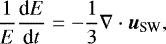
Knowing the shape and strength of the source as accurately as possible is important in order to normalise simulation results. In the case of solving the TPE by Parker (1965) by the means of SDEs, the relation appears as follows: instead of solving the TPE itself as a differential equation, a corresponding set of Langevin equations was solved as described, for instance, by Strauss et al. (2011a):
![Mathematical equation: \begin{equation*} \textrm{d}r =\left[\frac{1}{r^2}\frac{\partial}{\partial r}(r^2\kappa_{rr})+\frac{1}{r\sin\theta}\frac{\partial\kappa_{r\phi}}{\partial\phi}-u_{\textrm{SW}}\right]\textrm{d}s\\ +\sqrt{2\kappa_{rr}-\frac{2\kappa^2_{r\phi}}{\kappa_{\phi\phi}}}\textrm{d}\omega_r + \frac{\sqrt{2\kappa_{r\phi}}}{\kappa_{\phi\phi}}\textrm{d}\omega_{\phi}\\ \textrm{d}\theta=\left[\frac{1}{r^2\sin\theta}\frac{\partial}{\partial\theta}(\sin\theta\kappa_{\theta\theta})\right]\textrm{d}s + \frac{\sqrt{2\kappa_{\theta\theta}}}{r} \textrm{d}\omega_{\theta}\\ \textrm{d}\phi=\left[\frac{1}{r^2\sin^2\theta}\frac{\partial\kappa_{\phi\phi}}{\partial\phi}+\frac{1}{r^2\sin\theta}\frac{\partial}{\partial r}(r\kappa_{r\phi})\right]\textrm{d}s + \frac{\sqrt{2\kappa_{\phi\phi}}}{r\sin\theta}\textrm{d}\omega_{\phi}\\ \textrm{d}E=\left[\frac{1}{3r^2}\frac{\partial}{\partial r}(r^2 u_{\textrm{SW}})\Gamma E\right]\textrm{d}s{,} \end{equation*}](/articles/aa/full_html/2022/01/aa38980-20/aa38980-20-eq5.png) (1)
(1)
with Γ = (E + 2E0)∕(E + E0), κrr∕rϕ∕ϕϕ∕θθ being the entries of the diffusion tensor  in spherical coordinates aligned to the HMF as derived, for example, by Burger et al. (2000) and with d s being the time-backward time increment. The adiabatic energy changes are shown to only depend on the radial position due to the assumption made here of a constant, radial Solar wind speed, which is a reasonable assumption in the region and on the timescales of interest in the first part of this study (see, e.g. Köhnlein 1996). In order to solve Eq. (1), an iterative Euler-Maruyama scheme was used to solve these equations, which produces a set of random walk type solutions. This is due to the way in which the SDE approach treats the stochastic nature of diffusion by implementing a Wiener process
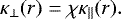
  , with ζ being a stochastic element as avector of Gaussian-distributed random numbers. The solutions can be described as point-like solutions of the time-dependent distribution function f(r, t), covering thewhole phase space as described by the TPE. As illustrated in Fig. 1, the temporal evolution of the solutions form trajectories through the phase space. In the case of a time-backward approach as utilised for this study (see e.g. Kopp et al. 2012; Strauss & Effenberger 2017), and depicted in Fig. 1, the injection point can be understood as the observational point and the phase-space trajectories follow a random walk to three possible sources, which are implemented as boundaryconditions. These, according to Dunzlaff et al. (2015), are firstly the Sun, indicated in yellow (such trajectories are neglected in this study due to the lack of a significant Solar component in high-keV and low-Mev energy range of electrons); the Jovian magnetosphere, indicated in orange (source spectrum according to Vogt et al. 2018); and the heliopause, indicated in blue (the local interstellar spectrum of galactic cosmic-ray electrons). Due to the time-backward approach, the number of particles which are injected at the observational points (and later evaluated) can be held constant, whereas the percentage which reaches the different boundaries varies depending on the propagation conditions.
Usually the point-like solutions of the SDEs in space and time are interpreted as a set of pseudo-particles. Thus, the phase-space trajectories, as illustrated in Fig. 1, could be understood to describe the propagation of particle samples. But this interpretation bears the problem that the solutions of the SDEs are inherently of a mathematical nature and could represent a varying number of physical particles (see Kopp et al. 2012; Strauss & Effenberger 2017; Vogt et al. 2020, amongst others). Therefore when we refer to the temporal evolution of the solutions in the following, we address them plainly as phase-space trajectories.
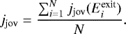
Since the phase space trajectories are mathematical solutions, they are – in contrast to a physical interpretation – equally probable. Inorder to be comparable with spacecraft data, a large number of phase space trajectories therefore have to be sampled and weighed according to their physical significance in order to approximate a spatial solution (see, e.g. Moloto et al. 2019). Thereby the corresponding source spectrum serves as a boundary weight (see, e.g. Strauss et al. 2011a; Kopp et al. 2012) in order to determine the contribution to the differential intensity as a physical quantity (or the physical likelihood of the phase space trajectory, respectively). As illustrated on the right side of Fig. 1, each radial step results in adiabatic energy losses (or gains in the time-backward approach) as obtained by the implementation of the modelling approach according to Eq. (1) until the boundary is reached. Subsequently, the trajectories are weighted by the source spectrum according to their exit energies Eexit and the number of phase-space trajectories N. Physically, this refers to the fact that the strength of the source indicates how likely a particle measured at the observational point with an initial energy Einit has left the source with Eexit. This means, as sketched by Fig. 1, that the phase-space trajectories effectively are weighted by the differential intensities at the source corresponding to their adiabatic energy gain which defines their energy at the source. In case of the Jovian source spectrum jjov(E), this leads to the expression
 (2)
(2)
The distribution function f is the solution of the TPE, and it is related to the differential intensity by j = P2f, where P = pc∕q is the rigidity of the electrons corresponding to the momentum p and the charge q, as well as to the speed of light c (see, e.g. Moraal 2013).
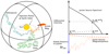 |
Fig. 1 Simulation setup according to Vogt et al. (2020). On the right side, a visualisation is shown of how the Jovian source spectrum determines the resulting differential intensity. The sketch thereby is to be read from bottom to top. The pseudo-particle was injected with an initial energy
|


2.3 The numerical setup
In an extension of the work presented in Vogt et al. (2020), the same SDE code as discussed by Dunzlaff et al. (2015) was utilised in order to perform the simulations. Since it is written in CUDA in order to optimise the performance time, several simplifications haven been made due to the limited internal memory on Graphic Processing Units (GPUs). The solar wind velocity was chosen to be directed radially outward and constant throughout the simulation setup. Following the deeper discussion on the parameter setting by Vogt et al. (2020), the value for this quantity was set to uSW= 400 km s−1, in agreement with solar minimum conditions. The corresponding HMF is assumed to be a Parker field. The HMF geometry enters into the transformation of the diffusion tensor, done here according to the approach of Burger et al. (2000). Thereby it is important to note that the HMF is only considered in this implicit way as parameters determining the geometry and values of the diffusion tensor and not implemented into the simulation setup itself, as done by a comparable finite difference scheme or magnetohydrodynamics (MHD) simulation setups. Furthermore, the geometry of the HMF is assumed as static throughout the simulation both as a whole and as well as regarding the individual field lines, effectively neglecting the Solar rotation. This approach is standard in Jovian transport studies and generally in cosmic ray modulation studies (see, e.g. Kota & Jokipii 1983; Ferreira & Potgieter 2002; Ferreira et al. 2003; Burger et al. 2008; Potgieter & Vos 2017). The effects of these simplifications on Jovian electron transport simulations are discussed by Vogt et al. (2020) and in more detail in Sect. 5.
The mean free paths determining the diffusion tensor are included and are based on the simplified, energy-independent approach applied successfully by e.g. Strauss et al. (2011a,b, among others): λ∥ was normalised at r0 = 1 AU, such that
 (3)
(3)
An energy dependence, however, does enter into the diffusion coefficient by way of its standard definition, viz. κ = vλ∕3 (see, e.g. Shalchi 2009), with v being the particle speed. Again following previous studies (e.g. Ferreira et al. 2001a,b), the perpendicular diffusion coefficient is assumed to be proportional to the parallel diffusion coefficient by a constant factor χ such that
 (4)
(4)
For the purposes of the present study, these simplified transport parameters serve to qualitatively emulate the behaviour in the inner heliosphere of more theoretically motivated expressions for the same employed in ab initio particle transport studies (see, e.g. Engelbrecht & Burger 2013; Engelbrecht 2019). For instance, the energy-independence of λ∥ over the range of (low) energies considered in this study reflects the behaviour of electron parallel mean free paths derived from quasilinear theory (see, e.g. Teufel & Schlickeiser 2003; Engelbrecht & Burger 2010; Dempers & Engelbrecht 2020), as well as what is expected from observations (e.g. Bieber et al. 1994). The energy-independent perpendicular mean free path was chosen to reflect the energy dependence expected from observational (e.g. Palmer 1982) and modulation studies (e.g. Burger et al. 2000)at the energies relevant to this study, and it does not differ much from the relatively weak energy dependences of perpendicular mean free paths derived from theory (see, e.g. Shalchi 2009; Burger et al. 2008; Engelbrecht & Burger 2015; Engelbrecht 2019).
Table 1 shows the choice of parameters used within this framework motivated and tested by Vogt et al. (2020). In order to do so, those authors performed a set of parameter studies varying the ‘computational’ parameters. The set of valueslisted in Table 1 was found to be a trustworthy compromise between the need to keep the simulation time low and to assure that the results are converging. Also the radius of the model setup RHP was specifically chosen because a smaller setup can influence the simulation results, as demonstrated by that study. The parallel mean free path λ∥ was determined by simulating the Jovian electron spectrum at Earth’s orbit during times of good magnetic connection at which the particle transport can be assumed to be dominated by parallel diffusion. Figure 2 shows the results of this study over an extended energy range, covering the whole range of interest of the Jovian source spectrum, as opposed to the single energy considered by Vogt et al. (2020). For the case of good magnetic connection to the source, the parallel mean free path λ∥ seems to be only slightly energy-dependent within the constraints of our modelling approach; although, in contrast to the limited energy range investigated by Vogt et al. (2020), λ∥ = 0.125 AU appears to be more in agreement with the simulation results covering the extended energy range. Therefore, the value listed in Table 1 appears to produce results that are most in agreement with spacecraft data at Earth’s orbit during comparable conditions. Likewise, χ was determined by applying the result for λ∥ and comparing the results of simulation runs with different values of χ to Jovian electron spectra obtained during times of poor magnetic connection as shown in Fig. 2b, where perpendicular diffusion is expected to be the predominant mechanism governing the transport of these electrons. As can be seen for both cases of λ∥ = 0.125 AU (second and third panel) and λ∥ = 0.15 AU (fourth and fifth panel), the energy dependence of χ is more prominent. It is worth noting that the decrease in χ is located in the keV-range. As discussed by Vogt et al. (2018), the Jovian source spectrum below the MeV range can only be determined by utilising Pioneer 10 flyby data by Teegarden et al. (1974), which has to be re-normalised, and SOHO data by Kühl et al. (2013) at Earth’s orbit, which shows a variation in its steepness below 1 MeV. These two uncertain influences on the source spectrum could translate into uncertainty about the behaviour of χ at these energies. In order to maximise the energy range with a physically reasonable choice, χ = 0.0125 was used for the simulation within this study, as listed alongside the other parameters in Table 1. The lack of energy dependence assumed in the simulation setup for the perpendicular mean free path λ⊥ is not expected to cause significant effects. As shown by Vogt et al. (2020), the range of exit energies which are significant in order to obtain the corresponding differential intensities is much smaller than the ones relevant for the energy dependence of χ in Fig. 2b.
Computational and physical parameters used for the code (when not stated otherwise).
2.4 The influence of boundary conditions
The effect of applying Eq. (2) is shown in Fig. 3. The panels on the left display the binned distribution of phase-space trajectories according to their exit energies for good (top panel) and poor magnetic connection to the source (middle panel) as well as the difference between them, assuming a Parker field geometry with a constant radial Solar wind speed. On the right side, the corresponding distributions are shown if Eq. (2) was applied and the phase-space trajectories were therefore weighted according to their physical significance. In both cases, the distributions were normalised to one. In order to interpret the results, particularly the relation between the distributions of the trajectories and the differential intensities, Fig. 3a displays an important feature: As marked by two dashed red lines, a sink in the intensity can be spotted throughout the whole energy range. It is important to note that it is directly located above the highest intensities shown by the phase-space trajectories, which are associated with very low energy gains. The comparison with Fig. 3c shows that the intensity sink in Fig. 3a appears where the phase-space distributions, in the case of poor magnetic connection to the source, become significant. This shift of the maximum of the distributions according to the magnetic connection to the source is also visible in Figs. 3b,d for the weighted contribution to the resulting differential intensities.
As noted above, both figures display the differences between the distributions, Fig. 3e showing the number of trajectories in each bin and Fig. 3f showing the sum of the weight of these trajectories according to the source spectrum. For both figures, the colour coding is defined symmetrically around zero. This highlights the important fact that despitesome negative bins in the difference distributions, which are mostly located within the area of the intensity sink, there is either an equal amount of entries or more bin entries (and therefore phase-space trajectories attributed to Jovian electrons) for the case of good magnetic connection to the Jovian source. While this in itself is an expectedresult (see Sect. 2.2), it is remarkable that the distinct maximum of this difference distribution is located below the intensity sink in Fig. 3a, which is indicated by two dashed red lines. Therefore the maximum below the intensity sink in Fig. 3a, which is identical to the population of phase-space trajectories responsible for almost the entire contribution to the resulting differential intensity according to Fig. 3b, has to be attributed to parallel diffusion-dominated transport. Since propagation parallel to the nominalParker spiral is the most effective mechanism for charged particle transport, it can be expected to be related to both shorter simulation times (i.e. amounts of random walk steps to perform the corresponding phase-space trajectory) as well as lower energy gains. That explains why this population of trajectories is absent in Fig. 3c, showing the phase-space trajectory distribution in the case of poor magnetic connection to the source.
We therefore interpret the simulation results as displayed in Fig. 3 as follows: Since the upper left triangle of the panels showing the phase-space trajectory distributions does not seem to vary with respect to the degree of magnetic connection, this population can be interpreted as a kind of diffusive background. By this, we aim to describe the fact that these trajectories appear to represent a population which exists, in a sense, independently of the physical propagation conditions pertaining to magnetic connectivity. This interpretation is further supported by the fact that, according to the corresponding panels on the right side of Fig. 3, this population has almost no physical significance with respect to the resulting differential intensities. Therefore it can be shown (see Vogt et al. 2020) that energy gains of more than half an order of magnitude most likely correspond to phase-space trajectories of low physical probability. With respect to Figs. 3e,f, we can conclude that the (physical) variation in intensities corresponding to changing magnetic connections between the observer and the source is caused by the (mathematical) variation of the maximum of the distribution of the phase-space trajectories below the intensity sink.
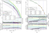 |
Fig. 2 Simulated Jovian electron spectra, similar to the figures by Vogt et al. (2020), but covering the whole energy range of the Jovian source where the energy range previously investigated by Vogt et al. (2020) is indicated by the two dashed blue lines. Top of the left panel: Earth orbit spectral data in the case of good connection to the source alongside with a data fit (dashed black line). The simulation results for different values of λ∥ = [0.05, 0.4] AU are colour coded. Middle panel: Fig. 2a shows the corresponding relative deviation to the source spectrum for both data and simulation results, with the area of a ± 0.5 deviationindicated in grey. Bottom panel: resulting energy dependence of the parallel mean free path. The right panel displays the corresponding results for different values of χ = [0, 0005, 0.045] in the case of a bad connection. Again, the top panels show the Earth orbit spectral data alongside a data fit indicated in a dashed black line. The relative deviations and resulting energy dependencies are shown for λ∥ = 0.125 AU (second and third panel) and λ∥ = 0.15 AU (fourth and fifth panel). |
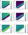 |
Fig. 3 Binned distributions of exit energies |

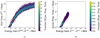 |
Fig. 4 Relation between the energy gain |


3 Modelling of residence times
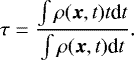
Within the mathematical framework of the Parker (1965) TPE, the residence time corresponding to the evolution of the probability density of the particles ρ is defined as the expectation value of the time according to
 (5)
(5)
As Vogt et al. (2020) point out, this approach cannot be transformed into SDE modelling by simply averaging over the pseudo-particles’ exit times. Instead, ρ is proposed to be the distribution of particle density as
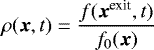 (6)
(6)
and normalised by the total phase-space density
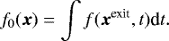 (7)
(7)
Thereby, f0(x) cancels out in Eq. (5). Applied to the discrete case of phase space trajectories as the output of an SDE code, Eq. (5) reads as
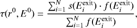 (8)
(8)
with s being the exit (integration) time corresponding to the different phase space trajectories. For a more detailed discussion of the derivation, see Sect. 3 of Vogt et al. (2020), especially Eqs. (7)–(10). Compared to the calculation of differential intensities by applying Eq. (2), this approach is self consistent, as each phase space trajectory is attributed the same significance due to it’s exit energy in both cases. We note for the further discussion in this paper that the exit energies are the results of the adiabatic energy changes experienced throughout the random walk which constitute the phase-space trajectories. Therefore the adiabatic energy changes define – in combination with the source spectrum as shown in Fig. 1 – the weight by which the exit times of the individual phase-space trajectories are taken into account. For 6 MeV Jovian electrons, Vogt et al. (2020) further show that the residence times obtained via Eq. (8) are between ~ 5− 11 days, depending on magnetic connectivity, and they are therefore shorter by almost two orders of magnitude when compared to previous estimations (see e.g. Strauss et al. 2011b; Vogt et al. 2020, and references therein).
3.1 Adiabatic energy changes and the role of the source spectrum
According to Eq. (8), the contribution of each phase-space trajectory depends on its exit time  , more precisely on the differential intensity
  corresponding to it within the source spectrum. We aim to investigate this relation further. Figure 4 shows the relation between the energy gain and the exit times of the phase space trajectories unweighted by Eq. (8) (Fig. 4a) and weighted by their contribution to the residence time (Fig. 4b) for the case of good magnetic connectivity between the Jovian source and the observer. As discussed above with reference to Fig. 3, the energy differences between the initial energies
  and the exit energies
  are caused by adiabatic energy changes as given by Parker (1965) within the TPE. For the SDEs’ modelling approach utilised here, the influence of this effect is included as follows: whereas each subsequent iteration of the random walk increases the corresponding simulation time si by the value of the time increment, the energy gain accompanying each step of the phase space trajectory is a function of energy and position. Therefore phase space trajectories of the same (time) length can be related to different rates of adiabatic energy changes Eexit − Einit as illustrated in the upper right part of Fig. 4a. As given by
 (9)
(9)
according to Parker (1965) and Webb & Gleeson (1979), the relation of adiabatic energy changes to simulation times is almost linear in the logarithmic display of Fig. 4b. Since Fig. 4a consists of the simulation results displayed with respect to their initial energies  in Fig. 3b, the intensity sink discussed in Sect. 2.2 also appears in Fig. 4a. The depiction (especially with respect to Fig. 4b) allows one to deduce that, according to the location of the intensity sink (red), phase-space trajectories corresponding to energy gains of more than half of an order of magnitude and a simulation time of more than eight days do not significantly contribute to the modelling results. This notion further supports the interpretation of Fig. 3 in Sect. 2.2 that this intensity sink segregates the physically significant population of phase-space trajectories from the (diffusive background) population, which is shown in Fig. 4a as a high energy gain and high exit time tail. The comparison with Fig. 4b validates this as the high energy gain and high exit time tail is shown to be weighted down to effectively zero by the boundary condition, that is the Jovian source spectrum.
These considerations suggest that the adiabatic energy changes implemented according to Eq. (9) always have to be considered in order to obtain physically reliable results as long as diffusive processes influence the particle’s propagation. As shown in Figs. 3 and 4 and discussed in detail in Sect. 2.2, the physical likeliness of (mathematically) equally possible phase-space trajectories is determined by the boundary conditions via the corresponding exit energy  . Therefore, not considering adiabatic energy changes effectively allows one to assume that the energy spectrum of the particle population of interest is flat, and therefore each energy is equally probable. This relation is also shown on the right side of Fig. 1. The following section further investigates the significant influence of the boundary conditions (and, by implication, adiabatic energy changes) on Jovian residence times over the whole Jovian energy range. Subsequently, these considerations and results will be applied to the analytical estimation of the GCR residence times as suggested by Parker (1965); O’Gallagher (1975); Strauss et al. (2011b), for example.
3.2 Adiabatic energy dependence of Jovian residence times
In also taking Fig. 5 into account in order to include the dependence of τ on the adiabatic energy changes, the intensity sink (as indicated in red) is confirmed over the whole energy range of interest. The right panels show the histograms for the exit times at the Jovian boundary considering each to be of equal probability, while the left panels show their contribution to the residence time according to Eq. (8). From top to bottom, first the case of good magnetic connectivity between the observer and the source is shown, followed by the case of poor magnetic connectivity and the difference of the two sets of histograms. Similar to Fig. 3e, which shows the difference of the phase-space trajectory distributions with respect to their corresponding exit energies, the difference of the phase-space trajectory distributions with respect to their corresponding exit times (Fig. 5e) also displays a significant maximum below the intensity sink (indicated in red). The comparison with Fig. 5f confirms that these trajectories indeed determine the residence time almost entirely. As discussed in detail above, this further supports that the population of pseudo-particles with trajectories dominated by the perpendicular diffusion process exit almost independently of the degree of magnetic connection between the source and the observer. However, the population corresponding to small exit times and low adiabatic energy gains seems to determine the resulting residence times, as it determines the resulting differential intensities. Since both small exit times and low adiabatic energy gains indicate very effective particle transport, it is reasonable to identify this population as being dominated by particles whose transport is governed by the parallel diffusion process as suggested by Vogt et al. (2020).
In the case of poor magnetic connection, however, Fig. 5c lacks the parallel diffusion-dominated population, but otherwise shows a similar shape. Again, the comparison with the corresponding contribution to the total differential intensity, as shown in Fig. 5d, suggests that the trajectories dominated by the perpendicular diffusion processes could be considered as being a ‘diffusive background’, since they neither change according to the degree of magnetic connection nor do they influence the physical results significantly. This is due to the fact that the pseudo-particles’ trajectories are the results of a Wiener process as the mathematical representation of Brownian motion. Although the concept of parallel diffusion mimics the actual physical particle motion in the case of good connectivity and therefore shows the significance illustrated by Figs. 5a,b, the results as a whole nevertheless have to be transformed according to Eq. (2) in order to assign a physically significant number of real particles to the pseudo-particles trajectories. This, as discussed in detail by Vogt et al. (2020), is of course equally applicable to the relation between the phase space trajectory exit times and the residence time as a result of applying Eq. (8).
The bottom panels of Fig. 5 confirm these assumptions: As demonstrated by Figs. 5e,f, the ‘diffusive background’ disappears almost entirely if only the differences between the histograms for good and poor connectivity are shown. Therefore the suggested interpretation would be that the possibility to reach the Jovian boundary via a perpendicular diffusion-dominated trajectory does not depend on the magnetic connectivity between the boundary and the start or observational point. The fact that the diffusive background appears to be invariant with respect to the magnetic connection between the observer and the source, however, shows that this population of phase-space trajectories is dominated by perpendicular diffusion since otherwise it would not have reached the Jovian source as a boundary. Only with increasingly good connectivity will the probability that trajectories dominated by parallel diffusion reach the boundary increase.
This effect is almost independent of the particle’s energy. Although Fig. 5a shows slightly shorter maxima of sexit for higher initial energies Einit, this effect is almost entirely limited to the population of trajectories which do not significantly contribute to the results. The most prominent energy-dependent effect appears to be the increasing density of the distributions in Fig. 5b, leading to more distinct maxima as is also slightly visible in Fig. 5a for the same exit times and initial energies, respectively. The fact that the intensity sink is present over the whole energy range further supports the interpretation of a ‘diffusive background’ and trajectories reflecting the physical behaviour of charged particles within the heliospheric magnetic field – as indicated by the fact that, in the case of good magnetic connection, only the latter population seems to contribute to the resulting differential intensity and residence times.
4 Comparison of numerical and analytical approaches
The large discrepancy between between the maxima of the distribution of the exit times sexit and the calculated residence times as displayed by the comparison in the left and right panels of Fig. 5 seems to be caused by the mathematical nature of the diffusion approach. As already outlined by Vogt et al. (2020) and discussed in Sect. 2.2 and especially Sect. 3.2 focussing on the role of adiabatic energy changes, the solutions of the SDE modelling approach (i.e. pseudoparticle trajectories) have to be transformed into physically meaningful quantities (i.e. differential intensities) by means of the source spectrum as a boundary condition. A probable consequence becomes apparent in comparison to the analytical approximations of Parker (1965) and O’Gallagher (1975). Comparing these analytical estimations to the results of our approach to simulate the residence times shows a pattern of deviations similar to the deviations of the exit time distributions.
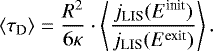
As the solution of the TPE is a four-dimensional probability density function of time, space, and rigidity (or energy, respectively), the residence time can be derived from it as the expectation value of the time as discussed at the beginning of Sect. 3 by means of Eq. (5). In order to solve the TPE analytically, however, it has to be simplified. Therefore, assumptions were made by Parker (1965) (and subsequently for all other analytical estimations so far as well) that κ and uSW are constant scalar values in time and space. Furthermore, it is assumed that the particles diffusion inwards are isotropic and that the particles propagate from the outer border of the heliosphere inwards towards its centre. Solving Eq. (5) under these assumptions yields a diffusion and a convection limit τD = R2∕(6κ) (see Parker 1965) and τC = R∕uSW (see O’Gallagher 1975), respectively. For a more detailed description of the derivation, see also Strauss et al. (2011a), and references therein. Evidently, both estimations are independent of the particle energy. The diffusion limit τD, however, incorporates an indirect dependence via the overall average value of the diffusion coefficient κ. The assumption of a globally constant value of κ, which does not depend on the radial distance nor differentiates between parallel and perpendicular diffusion processes, of course is not realistic for the case of Jovian electrons, which have transport properties that strongly depend on whether parallel or perpendicular diffusion dominates. Therefore Galactic electrons have to be taken into account in order to compare these estimations with simulation results.
For the purpose of these qualitative considerations, we used the galactic electron LIS proposed by Potgieter et al. (2015) in order to apply Eq. (8) to the phase space trajectories exiting at the outer boundary equivalent to the way the Jovian residence times are calculated. Although the same transport processes also govern the propagation of GCR electrons, their isotropic influx allows one to roughly combine parallel and perpendicular diffusion into one effective value of κ according to Parker (1965), for example. Nevertheless the results of Strauss et al. (2011b, 2013), who benchmarked their numerical estimation in the case of GCR electrons against the analytical diffusion limit τD by Parker (1965, 1966) and a combined estimation of 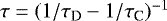 , show in the Jovian electron case that values of λ∥ = λ⊥≈ 1 AU are required in order to obtain realistic values for the Jovian residence times, a result which is in contrast to values successfully employed in modulation studies by, for example, Ferreira et al. (2001a,b), Kissmann et al. (2004), Sternal et al. (2011), Strauss et al. (2011a), and Nndanganeni & Potgieter (2016), amongst others, as well as in contrast to what is expected from theory (e.g. Engelbrecht & Burger 2013; Dempers & Engelbrecht 2020; Shalchi 2020) and numerical test-particle simulations of diffusion coefficients (e.g. Minnie et al. 2007; Heusen & Shalchi 2016; Dundovic et al. 2020). It is important to note that the increase in the mean free paths with radial distance has to be balanced with the fact that also the much less effective perpendicular diffusion has to be considered. Therefore, the assumption that λ∥ = λ⊥≈ 1 AU, which is almost an order of magnitude larger than the parallel mean free path at Earth’s orbit (see, e.g. Bieber et al. 1994) and almost three orders of magnitude larger than the perpendicular mean free path (see, e.g. Palmer 1982; Giacalone 1998), appears to be unrealistic.
This discrepancy is most likely caused by the fact that neither of the analytical estimates incorporate the adiabatic energy changes and, therefore, to a degree they neglect the boundary conditions. As argued above in Sect. 3.1, the TPE is solved for an isotropic diffusion approach and a flat energy spectrum as input. This simplification appears to be problematic because it neglects the physical constraints of charged particle transport theory. Most significantly, it should be noted that the diffusive processes incorporated into the TPE describe stochastic processes associated with (pitch-angle) scattering at irregularities within the HMF, as acknowledged by Parker (1965). The effect of the source spectrum as the boundary condition included via the adiabatic energy changes is discussed in Sect. 2.2, explained in great detail by Vogt et al. (2020), and illustrated in Fig. 1. Summarised, and put in mathematical terms, the analytical estimates by Parker (1965), O’Gallagher (1975), and Strauss et al. (2011b) are the temporal expectation value of the probability density function and, as the boundary conditions are neglected, not of the corresponding differential intensity. In order to avoid the consequences of over-simplifying within the analytical estimates by neglecting the boundary conditions and neglecting realistic diffusion conditions, it therefore seems to be necessary to incorporate an analytical estimate of the effect of boundary conditions.
Indeed, Fig. 6 shows that the main effect of weighting the trajectories according to their contribution to the differential intensity determines the results for the Galactic population as well. As one would expect, the analytical estimation of τd according to Parker (1965) (dashed white and black line) in Fig. 6a is in agreement with the unweighted distribution of exit times. The numerical estimation according to Vogt et al. (2020), however, strongly deviates in this case, as shown by the red dashed line, which is similar to the case of the Jovian electron population. These findings confirm our interpretation of the significance of including the boundary conditions via the adiabatic energy changes in order to transform the mathematical solution of the TPE into a physical and observationally meaningful one. Due to the adiabatic energy changes of particles, they are not detected with the energy they had at their source. In order to calculate the residence time of a particle detected with Einit = 6 MeV at the observational point, one therefore would have to assume an energy of Eexit = Einit + ΔE at the source with ΔE being the average adiabatic energy change of the particle population. Since these two energies correspond to different intensities if the spectrum is not assumed to be flat (as is assumed here on the basis of observations, see the discussion in Sect. 3.1), the adiabatic energy changes can be transformed into intensity changes within this mathematical framework. Neglecting the influence of adiabatic energy changes would implicitly assume an energy-independent source spectrum.
The approach to estimate the characteristic energy change as being proportional to the initial energy is supported by Parker (1965), who assumed the energy loss after a time t as being given by
 (10)
(10)
and that t is not energy-dependent. Solving a simplified TPE accordingly, this approach leads to an average fractional energy loss of
 (11)
(11)
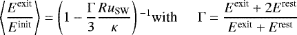
as derived by Parker (1966). As pointed out by Strauss et al. (2011b), for example, this expression is only valid for a constant stream of inflowing particles with a globally constant mean free path and diffusion tensor, respectively. Figure 7 shows the analytical estimate of the diffusion limit τ alongside its corrected value according to both estimates for the adiabatic energy changes, Eqs. (10) and (11). As outlined above in the second paragraph of this section, we therefore assumed the analytical estimate of the effect of the boundary conditions to be a function of the ratio of the source spectrum intensity jLIS(E) at the initial energy Einit and at the exit energy Eexit, given by:
 (12)
(12)
A limitation of this approach is that only the diffusive limit τD is considered. The approach by Strauss et al. (2011b), which also considers the outward convection of the particles, is not defined for the small values of λ, and therefore of κ, that we need to apply for Jovian electrons as shown and discussed in Sect. 2.3 and Vogt et al. (2020). Nevertheless the slightly lower values of τD (see Strauss et al. (2011b) fora detailed discussion) appear to be in agreement with the exit times sexit as displayed in Fig. 6a. As illustrated by Fig. 7, the explicit analytical solution for the fractional adiabatic energy loss given by Eq. (11) is also not physically, usefully defined due to the unrealistic assumption made in its derivation that RHP∕κ ≪ 1, given that the Voyager mission confirmed that RHP ≈ 120 AU (see e.g. Gurnett et al. 2013; Krimigis et al. 2013; Stone et al. 2019) and that our results for λ∥∕⊥ suggest significantly smaller values for κ.
Therefore, as indicated by the wider range of definitions in Fig. 7, we have to choose to apply Eq. (10) in order to estimate the effect of the boundary conditions on the analytical estimate for the residence time, otherwise our value for λ would be outside the range covered by the assumptions. As the energy E(t) in Eq. (10) is given depending on the time t and the energy E0 with which the particle enters the heliosphere, Eq. (10) has to be rewritten according to the time-backward approach, and we therefore have to compare our analytical estimate with the following:
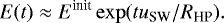 (13)
(13)
Since we are interested in the total average energy gain for GCR electrons, we substituted t with the diffusion limit  and obtained
 (14)
(14)
As indicated by Eq. (9), the adiabatic energy changes are more effective when the radial distance at which the particle finds itself is lower. Therefor, we assume the value of κ to correspond to the value of the parallel mean free path λ∥ = 0.125 AU at Earth’s orbit (marked in red in Fig. 7). Furthermore, the analytical estimates cannot distinguish between perpendicular and parallel diffusion. Therefore, κ not only has to incorporate the effective diffusion parallel to the magnetic field, but also the diffusion perpendicular to the field lines, which is less effective by almost two orders of magnitude as shown by the value of χ in Table 1. Due to the much longer path length of the Parker spiral in comparison with the radial distance, the more ineffective perpendicular transport cannot be ignored. Our assumptions are supported by Fig. 6a as it shows that the similarly calculated diffusion limit  is in agreement with the simulation results. Despite being located at the lower edge of the definition range and the uncertainties implicit for the need to assume an effective global value of κ, Fig. 7 supports the qualitative notion that the effect of the boundary conditions can be estimated as being a factor of 1∕3 to 1∕4, as indicated bythe black and white dashed lines in Fig. 6b.
We can demonstrate that this analytical estimation shifts to the same range of values as suggested by our numerical estimation given by Eq. (8) and indicated by the dashed red line. While a more detailed treatment of how to define and derive a characteristic energy change is beyond the scope of this study, the approach provided herein should be sufficient to qualitatively strengthen our point as to how diffusion and adiabatic energy changes are physically interlinked with each other within the theoretical treatment of charged particle transport. As described by Vogt et al. (2020), the approach to model diffusion via a Wiener process does not track the particle motion itself, leading to mathematical remnants such as the ’diffusive background’ as discussed in Sects. 2.2 and 3.2, which then have to be transformed into physically useful solutions by convolution with the source spectrum. The comparison between analytical and numerical estimations, however, suggests that these considerations apply to diffusion as a mathematical model to treat particle motion in general, rather than just to its numerical implementation by means of SDEs.
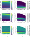 |
Fig. 5 Binned distributions of exit times over the whole energy range dominated by Jovian electrons, displayed similarly in Fig. 3. Whereas the right panels show the exit time distributions weighted by their contribution according to Eq. (8), the left side displays the unweighted results of the simulation. The first row (a,b) shows the distributions for the case of good magnetic connection, and the second for the case of poor connection. e,f: differences between the distributions for good and poor magnetic connection, highlighting the influence of magnetic connectivity on the simulation results. |
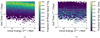 |
Fig. 6 Similar to Fig. 5, but for trajectories exiting at the outer boundary are shown instead of the Jovian magnetosphere. Left panel: distribution of unweighted exit times
|

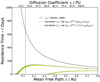 |
Fig. 7 Analytical estimate of the GCR residence time according to Parker (1965) with respect to the assumed mean free path λ (bottom x-axis) and the resulting diffusion coefficient κ (top x-axis).The two dashed lines show the corrected analytical estimates according to the estimations for the adiabatic energy loss by Eqs. (10) and (11), respectively. The resulting residence times are shown, colour coded from blue to yellow, for the whole energy range of the Jovian spectrum (by 30 logarithmically spaced representive energies) as a measure of the uncertainty. |
5 Corotational effects as possible measure
One way to examine these considerations is to utilise the corotational effects described by Vogt et al. (2020). As described in Sect. 2.3, the HMF is considered only by its geometry and not directly implemented itself. Because the Solar rotation is also neglected by the simulation setup, the magnetic connection between the Jovian source and the observer does not change throughout the simulation – or put more explicitly, for the duration of each simulation run, the observer is located on the same Parker magnetic field line. In order to investigate the effects caused by these simplifications, Vogt et al. (2020) implemented the effect of the Solar rotation (and therefore the co-rotation of the HMF) by considering the longitudinal motion of the Jovian source relative to the static HMF geometry. Comparing simulations over the whole longitudinal range with both a static Jovian source and a co-rotating one reveals a significant deviation of about 50° from the nominally best-connected longitude, an effect even larger in the case of a poor magnetic connection between the observer and the Jovian source. Utilising simulation results from Vogt et al. (2020), Fig. 8 shows the physical mechanism behind this. Two different effects determine the magnetic connection between Jupiter and a possible observer:
- 1.
The synodic period, in case of Earth, the characteristic ≈13 months first discussed by McDonald et al. (1972).
- 2.
The corotation of the HMF due to the Sun’s rotational period of ΩS ≈ 27 days.
The synodic corotation of ≈13 months bears more or less no detectable effect since the expected angular shift between Earth and Jupiter in the case of good magnetic connectivity is about Δϕ ≾ 4°. The angular speed of the HMF caused by the Solar rotation with ΩS ≈ 27 days, however, suggests a much more significant angular deviation of Δϕ ≿ 50°, which was confirmed via the simulation by Vogt et al. (2020). The corresponding relative motion between the HMF and the Jovian source thereby was implemented as a co-rotation of Jupiter by an additional term in the longitudinal SDE as given by Eq. (1). A similar approach was taken by Ferreira (2002). The deviation of the maximum intensity from the nominally best-connected longitude caused by this adjustment of the simulation setup is indicated by the red shaded shift in Fig. 8. As illustrated in the left panel of Fig. 8, the reason for this shift is the following: Due to the Sun’s angular rotation, the nominal Parker-like HMF frozen into the radially outward streaming Solar wind also rotates with the same angular velocity. During the propagation of Jovian electrons (indicated for good and poor connections by the orange trajectories in Fig. 8), a Parker-spiral connecting the Jovian source with the Earth orbit (dashed black circle) would change its longitudinal position, as indicated by the red arrow. Since the Jovian electron could follow the path of the nominal Parker-spiral by the more effective processes categorised as parallel diffusion (indicated by the larger step sizes inFig. 8), the residence times in the case of good magnetic connection are small and only cause small corotation effects. For the case of poor magnetic connection, however, perpendicular diffusion dominates the propagation processes of Jovian electrons that happen to reach the observer at Earth’s orbit and, therefore, it leads to much longer residence times. As indicated by the blue arrow and the blue shaded area in Fig. 8, respectively, the corresponding angular shift of the mininum of the 13 month periodicity of Jovian electron intensity is expected to be much larger. However, due to the longer residence times, the fluctuations in both Solar wind speed and the HMF can be expected to significantly interfere with this effect. But even in the case of good magnetic connection, the angular shift due to the corotation is expected to be large enough to be possibly resolved by spacecraft data and therefore could serve as an (indirect) measure for the residence time via
 (15)
(15)
with ΩS being the Sun’s angular speed. Although conceptually simple, this approach brings about several difficulties concerning the data analysis it requires. Despite being generally difficult to detect (see e.g. Heber et al. 2005, among others), electron counting rates are often highly influenced by Solar Energetic Particles (SEP) events and Corotating Interaction Regions (CIRs). Furthermore the HMF, as defined by Parker (1958) and used by the modelling setup (see Sect. 2.3 as well as Dunzlaff et al. 2015; Vogt et al. 2020), assumes a globally constant solar wind velocity, which is a strong simplification of the longer timescales involved, even during periods of low solar activity.
Figure 9 therefore shows SOHO-EPHIN electron data covering four synodic periods between 2006–2011, plotted with regard to their longitudinal separation from the nominal angle of best connectivity. The HMF for this matter was assumed to be frozen into a solar wind with a radial speed of uSW = 400 km s−1. In order to constrain the database to the boundaries given by means of the simulation setup, daily differential electron intensities were only included if all hourly averages of the solar speed by SOHO-CELIAS were within the range of [300, 400] km s−1. The remaining daily averages of solar wind speeds are plotted in the lower panel of Fig. 9. The corresponding electron intensities of the E300 (blue) and E1300 (orange) channels of the EPHIN instrument still show a large range of variation but an envelope in agreement with the simulation results. This can be understood by way of how solar wind speed variations influence the propagation between the Jovian source and the observer. By choosing only days with solar wind speeds with hourly averages not bigger than uSW = 400 km s−1, we assure that these variations change the longitude of best connectivity due to the decreases in the solar wind speed, resulting in a shift to the right seen in Fig. 9. The effect of these shifts of connectivity is a change in the corresponding electron intensity.
If the observers were well connected to the Jovian source by a HMF corresponding to uSW = 400 km s−1, a decrease in the solar wind speed would lead to a loss of connectivity and the Jovian electron intensity would likewise decrease. Thus only the upper envelope of the data is comparable to the simulations with an undisturbed HMF. Another reason to limit the focus on the envelope as a test of principle is the fact that the Solar wind takes several days to propagate across the 4 AU between Earth and Jupiter. Thus to be in complete agreement with the simulation, we would have needed data corresponding to days of stable Solar wind conditions. Since Fig. 9 already displays five years of data during the most stable conditions measured by SOHO-EPHIN, this simply is a problem of statistics. But as shown in the upper panel of Fig. 9, both of the electron channels of EPHIN meet the theoretical and computational expectations within the restrictions described. While the simulation results are in agreement, both qualitatively and quantitatively, with observations from the E300 channel, the intensities provided by E1300 are higher than expected. There are two possible reasons for this divergence. In order to calculate a representative energy for each channel, the detector responses (see Kühl et al. 2013) have to be convoluted with the electron spectrum. Apart from these technical difficulties, the Galactic component could also contribute to the measured energies more significantly than expected, despite the results of Nndanganeni & Potgieter (2018) who suggest that there is no significant Galactic electron contribution up to measured energies of ≈ 25 MeV. In addition to these possible statistical causes, another reason for the deviation could be the fact that, due to smaller fluxes, the unstable HMF conditions as described above could, in general, have a larger impact on the data.
Nevertheless, the fact that the envelopes of both electron channels plotted in Fig. 9 are in agreement with both the simulation results and the theoretical expectation can be considered as a confirmation of concept. Despite the uncertainties tied to the fluctuation in the propagation conditions, this result serves as encouragement to investigate this approach further when future spacecraft missions may provide data with improved statistics.
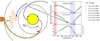 |
Fig. 8 Differential intensities of Jovian electrons for different initial energies Einit. Top panel: longitudinal variation due to varying connection for a co-rotating Jovian source. Middle panel shows the case of a static Jupiter. Bottom panel: ratio of the results of the two approaches. The right panel is taken from Vogt et al. (2020). |
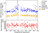 |
Fig. 9 Effect of corotation as shown in Fig. 8 as detected by SOHO-EPHIN. While the upward pointing and downward pointing triangles mark the positions of the maxima and minima of the simulated Jovian fluxes, as shown in the upper panel of Fig. 8, the two electron channels are shown in blue and orange as daily averages sampled over four synodic periods during the 2006–2011 Solar minimum. The simulation results corresponding to initial energies equivalent to those of theelectron channels are shown to match to the envelope of the data. In the lower panel, the corresponding SOHO-CELIAS data points are given for the daily averages of the Solar wind speed. Both panels show their data with respect to the longitudinal separation to the nominal point of best magnetic connection. |
6 Discussion and conclusions
This paper has investigated the energy dependence of residence times, focussing on the effect that adiabatic energy changes have on the mathematical implementation of diffusion. We have discussed how adiabatic energy changes and simulation times are related within the framework of SDE modelling. These considerations in Sect. 3.2 were taken into account in order to investigate how different initial energies Einit influence the estimated residence times according to Fig. 5. The significant features of the results (both weighted and unweighted for good and poor magnetic connection) were used to further explore how the mathematical results are related to the physically observable quantities.
This question initially led to the suggestion to calculate residence times as proposed by Vogt et al. (2020) and outlined in Sect. 3, but it appears to be of broader significance. As we showed by comparing the numerical and analytical approaches concerning the residence times of GCRs, the prior analytical approaches to estimate residence times are equivalent to taking the simulation or exit times sexit as a measure for τ. Therefore this study provides evidence to include representative adiabatic energy changes in the analytical approach. As discussed in Sects. 3.2 and 4, it has long been established that the convolution with the source (or equivalent boundary conditions in a non-time-backward SDE approach) is necessary in order to transform the results of a diffusion equation describing Brownian motion into a physically relevant solution of a more complex stochastic process. By means of Eq. (12), we suggest a simple but sufficient approximation which appears to reproduce the simulation results and could further serve as a more reliable first estimate for residence times when simulation results are not available.
Utilising the fact that the residence times result in a longitudinal shift of the best magnetic connection to the Jovian source due to relative orbital motions, as discussed in Sect. 5, we are able to show via Fig. 9 that our estimations are in general agreement with the observable longitudinal dependence of electron intensities. Since the estimation of residence times is connected to adiabatic energy changes (and therefore spectral modulation) as well as the transport parameters within the TPE, this offers a further possibility to constrain charged particle transport simulations. An example of this is the investigation of CIRs and their effect on particle propagation. The questions as to whether and how the considerations and results of this study can be generalised and applied to focussed transport equations describing SEP events, among others, is beyond the scope of this work, but it appears to be a promising task for subsequent research.
Acknowledgements
This work is based on the research supported in part by the National Research Foundation of South Africa (Grant Number 111731). Opinions expressed and conclusions arrived at are those of the author and are not necessarily to be attributed to the NRF. K.H. gratefully acknowledges the support from the German Research Foundation (Deutsche Forschungsgemeinschaft, DFG) priority program SPP 1992 “Exploring the Diversity of Extrasolar Planets” through the project HE 8392/1-1, and further likes to thank ISSI and the supported International Team 464 (ETERNAL).
References
- Baker, D. N., & van Allen, J. A. 1976, J. Geophys. Res., 81, 617 [NASA ADS] [CrossRef] [Google Scholar]
- Bieber, J. W., Matthaeus, W. H., Smith, C. W., et al. 1994, ApJ, 420, 294 [Google Scholar]
- Burger, R. A., Potgieter, M. S., & Heber, B. 2000, J. Geophys. Res., 105, 27447 [NASA ADS] [CrossRef] [Google Scholar]
- Burger, R. A., Krüger, T. P. J., Hitge, M., & Engelbrecht, N. E. 2008, ApJ, 674, 511 [NASA ADS] [CrossRef] [Google Scholar]
- Chenette, D. L., Conlon, T. F., Pyle, K. R., & Simpson, J. A. 1977, ApJ, 215, L95 [NASA ADS] [CrossRef] [Google Scholar]
- Conlon, T. F. 1978, J. Geophys. Res., 83, 541 [NASA ADS] [CrossRef] [Google Scholar]
- Dempers, N., & Engelbrecht, N. E. 2020, Adv, Space Res., 65, 2072 [NASA ADS] [CrossRef] [Google Scholar]
- Dundovic, A., Pezzi, O., Blasi, P., Evoli, C., & Matthaeus, W. H. 2020, Phys. Rev. D, 102, 103016 [NASA ADS] [CrossRef] [Google Scholar]
- Dunzlaff, P., Strauss, R. D., & Potgieter, M. S. 2015, Comput. Phys. Commun., 192, 156 [NASA ADS] [CrossRef] [Google Scholar]
- Engelbrecht, N. E. 2019, ApJ, 872, 124 [NASA ADS] [CrossRef] [Google Scholar]
- Engelbrecht, N. E., & Burger, R. A. 2010, Adv. Space Res., 45, 1015 [NASA ADS] [CrossRef] [Google Scholar]
- Engelbrecht, N. E., & Burger, R. A. 2013, ApJ, 779, 158 [NASA ADS] [CrossRef] [Google Scholar]
- Engelbrecht, N. E., & Burger, R. A. 2015, ApJ, 814, 152 [NASA ADS] [CrossRef] [Google Scholar]
- Eraker, J. H. 1982, ApJ, 257, 862 [NASA ADS] [CrossRef] [Google Scholar]
- Ferreira, S. E. S. 2002, PhD thesis, North-West University, South Africa [Google Scholar]
- Ferreira, S. E. S., & Potgieter, M. S. 2002, J. Geophys. Res. Space Phys., 107, 1221 [Google Scholar]
- Ferreira, S. E. S., Potgieter, M. S., Burger, R. A., Heber, B., & Fichtner, H. 2001a, J. Geophys. Res., 106, 24979 [NASA ADS] [CrossRef] [Google Scholar]
- Ferreira, S. E. S., Potgieter, M. S., Burger, R. A., et al. 2001b, J. Geophys. Res., 106, 29313 [CrossRef] [Google Scholar]
- Ferreira, S. E. S., Potgieter, M. S., Moeketsi, D. M., Heber, B., & Fichtner, H. 2003, ApJ, 594, 552 [NASA ADS] [CrossRef] [Google Scholar]
- Fichtner, H., Potgieter, M., Ferreira, S., & Burger, A. 2000, Geophys. Res. Lett., 27, 1611 [CrossRef] [Google Scholar]
- Florinski, V., & Pogorelov, N. 2009, ApJ, 701, 642 [CrossRef] [Google Scholar]
- Giacalone, J. 1998, Space Sci. Rev., 83, 351 [NASA ADS] [CrossRef] [Google Scholar]
- Gurnett, D. A., Kurth, W. S., Burlaga, L. F., & Ness, N. F. 2013, Science, 341, 1489 [NASA ADS] [CrossRef] [Google Scholar]
- Heber, B., Kopp, A., Fichtner, H., & Ferreira, S. E. S. 2005, Adv. Space Res., 35, 605 [NASA ADS] [CrossRef] [Google Scholar]
- Heusen, M., & Shalchi, A. 2016, Ap&SS, 361, 308 [NASA ADS] [CrossRef] [Google Scholar]
- Kissmann, R., Fichtner, H., Heber, B., Ferreira, S., & Potgieter, M. 2003, Adv. Space Res., 32, 681 [NASA ADS] [CrossRef] [Google Scholar]
- Kissmann, R., Fichtner, H., & Ferreira, S. E. S. 2004, A&A, 419, 357 [NASA ADS] [CrossRef] [EDP Sciences] [Google Scholar]
- Köhnlein, W. 1996, Sol. Phys., 169, 209 [CrossRef] [Google Scholar]
- Kopp, A., Büsching, I., Strauss, R. D., & Potgieter, M. S. 2012, Comput. Phys. Commun., 183, 530 [NASA ADS] [CrossRef] [Google Scholar]
- Kota, J., & Jokipii, J. R. 1983, ApJ, 265, 573 [NASA ADS] [CrossRef] [Google Scholar]
- Krimigis, S. M., Decker, R. B., Roelof, E. C., et al. 2013, Science, 341, 6142 [Google Scholar]
- Kühl, P., Dresing, N., Dunzlaff, P., et al. 2013, Proceedings of 33th International Cosmic Ray Conference (ICRC 2013), 3480 [Google Scholar]
- McDonald, F. B., Cline, T. L., & Simnett, G. M. 1972, J. Geophys. Res., 77, 2213 [NASA ADS] [CrossRef] [Google Scholar]
- Minnie, J., Bieber, J. W., Matthaeus, W. H., & Burger, R. A. 2007, ApJ, 663, 1049 [NASA ADS] [CrossRef] [Google Scholar]
- Moloto, K. D., Engelbrecht, N. E., Strauss, R. D., Moeketsi, D. M., & van den Berg, J. P. 2019, Adv. Space Res., 63, 626 [NASA ADS] [CrossRef] [Google Scholar]
- Moraal, H. 2013, Space Sci. Rev., 176, 299 [CrossRef] [Google Scholar]
- Nndanganeni, R. R., & Potgieter, M. S. 2016, Adv. Space Res., 58, 453 [NASA ADS] [CrossRef] [Google Scholar]
- Nndanganeni, R. R., & Potgieter, M. S. 2018, Astrophys. Space Sci., 363, 156 [NASA ADS] [CrossRef] [Google Scholar]
- O’Gallagher, J. J. 1975, ApJ, 197, 495 [CrossRef] [Google Scholar]
- Palmer, I. D. 1982, Rev. Geophys. Space Phys., 20, 335 [Google Scholar]
- Parker, E. N. 1958, ApJ, 128, 664 [Google Scholar]
- Parker, E. N. 1965, Planet. Space Sci., 13, 9 [Google Scholar]
- Parker, E. N. 1966, Planet. Space Sci., 14, 371 [NASA ADS] [CrossRef] [Google Scholar]
- Pei, C., Bieber, J. W., Burger, R. A., & Clem, J. 2010, J. Geophys. Res. Space Phys., 115, A3 [Google Scholar]
- Potgieter, M. S. 1996, J. Geophys. Res., 101, 24411 [NASA ADS] [CrossRef] [Google Scholar]
- Potgieter, M. S., & Vos, E. E. 2017, A&A, 601, A23 [NASA ADS] [CrossRef] [EDP Sciences] [Google Scholar]
- Potgieter, M. S., Vos, E. E., Munini, R., Boezio, M., & Di Felice, V. 2015, ApJ, 810, 141 [NASA ADS] [CrossRef] [Google Scholar]
- Pyle, K. R., & Simpson, J. A. 1977, ApJ, 215, L89 [NASA ADS] [CrossRef] [Google Scholar]
- Shalchi, A., 2009, Astrophysics and Space Science Library (Berlin: Springer), 362 [Google Scholar]
- Shalchi, A. 2020, Space Sci. Rev., 216, 23 [NASA ADS] [CrossRef] [Google Scholar]
- Sternal, O., Engelbrecht, N. E., Burger, R. A., et al. 2011, ApJ, 741, 23 [NASA ADS] [CrossRef] [Google Scholar]
- Stone, E. C., Cummings, A. C., Heikkila, B. C., & Lal, N. 2019, Nat. Astron., 3, 1013 [NASA ADS] [CrossRef] [Google Scholar]
- Strauss, R. D. T., & Effenberger, F. 2017, Space Sci. Rev., 212, 151 [CrossRef] [Google Scholar]
- Strauss, R. D., Potgieter, M. S., Büsching, I., & Kopp, A. 2011a, ApJ, 735, 83 [NASA ADS] [CrossRef] [Google Scholar]
- Strauss, R. D., Potgieter, M. S., Kopp, A., & Büsching, I. 2011b, J. Geophys. Res. Space Phys., 116, A12105 [Google Scholar]
- Strauss, R. D., Potgieter, M. S., & Ferreira, S. E. S. 2013, Adv. Space Res., 51, 339 [NASA ADS] [CrossRef] [Google Scholar]
- Teegarden, B. J., McDonald, F. B., Trainor, J. H., Webber, W. R., & Roelof, E. C. 1974, J. Geophys. Res., 79, 3615 [NASA ADS] [CrossRef] [Google Scholar]
- Teufel, A., & Schlickeiser, R. 2003, A&A, 397, 15 [NASA ADS] [CrossRef] [EDP Sciences] [Google Scholar]
- Vogt, A., Heber, B., Kopp, A., Potgieter, M. S., & Strauss, R. D. 2018, A&A, 613, A28 [NASA ADS] [CrossRef] [EDP Sciences] [Google Scholar]
- Vogt, A., Engelbrecht, N. E., Strauss, R. D., et al. 2020, A&A, 642, A170 [NASA ADS] [CrossRef] [EDP Sciences] [Google Scholar]
- Webb, G. M., & Gleeson, L. J. 1979, Astrophys. Space Sci., 60, 335 [NASA ADS] [CrossRef] [Google Scholar]
- Zhang, M. 1999, ApJ, 513, 409 [NASA ADS] [CrossRef] [Google Scholar]
- Zhang, M., Qin, G., Rassoul, H., et al. 2007, Planet. Space Sci., 55, 12 [NASA ADS] [CrossRef] [Google Scholar]
All Tables
Computational and physical parameters used for the code (when not stated otherwise).
All Figures
|
Fig. 1 Simulation setup according to Vogt et al. (2020). On the right side, a visualisation is shown of how the Jovian source spectrum determines the resulting differential intensity. The sketch thereby is to be read from bottom to top. The pseudo-particle was injected with an initial energy
|
| In the text | |
|
Fig. 2 Simulated Jovian electron spectra, similar to the figures by Vogt et al. (2020), but covering the whole energy range of the Jovian source where the energy range previously investigated by Vogt et al. (2020) is indicated by the two dashed blue lines. Top of the left panel: Earth orbit spectral data in the case of good connection to the source alongside with a data fit (dashed black line). The simulation results for different values of λ∥ = [0.05, 0.4] AU are colour coded. Middle panel: Fig. 2a shows the corresponding relative deviation to the source spectrum for both data and simulation results, with the area of a ± 0.5 deviationindicated in grey. Bottom panel: resulting energy dependence of the parallel mean free path. The right panel displays the corresponding results for different values of χ = [0, 0005, 0.045] in the case of a bad connection. Again, the top panels show the Earth orbit spectral data alongside a data fit indicated in a dashed black line. The relative deviations and resulting energy dependencies are shown for λ∥ = 0.125 AU (second and third panel) and λ∥ = 0.15 AU (fourth and fifth panel). |
| In the text | |
|
Fig. 3 Binned distributions of exit energies |
| In the text | |
|
Fig. 4 Relation between the energy gain |
| In the text | |
|
Fig. 5 Binned distributions of exit times over the whole energy range dominated by Jovian electrons, displayed similarly in Fig. 3. Whereas the right panels show the exit time distributions weighted by their contribution according to Eq. (8), the left side displays the unweighted results of the simulation. The first row (a,b) shows the distributions for the case of good magnetic connection, and the second for the case of poor connection. e,f: differences between the distributions for good and poor magnetic connection, highlighting the influence of magnetic connectivity on the simulation results. |
| In the text | |
|
Fig. 6 Similar to Fig. 5, but for trajectories exiting at the outer boundary are shown instead of the Jovian magnetosphere. Left panel: distribution of unweighted exit times
|
| In the text | |
|
Fig. 7 Analytical estimate of the GCR residence time according to Parker (1965) with respect to the assumed mean free path λ (bottom x-axis) and the resulting diffusion coefficient κ (top x-axis).The two dashed lines show the corrected analytical estimates according to the estimations for the adiabatic energy loss by Eqs. (10) and (11), respectively. The resulting residence times are shown, colour coded from blue to yellow, for the whole energy range of the Jovian spectrum (by 30 logarithmically spaced representive energies) as a measure of the uncertainty. |
| In the text | |
|
Fig. 8 Differential intensities of Jovian electrons for different initial energies Einit. Top panel: longitudinal variation due to varying connection for a co-rotating Jovian source. Middle panel shows the case of a static Jupiter. Bottom panel: ratio of the results of the two approaches. The right panel is taken from Vogt et al. (2020). |
| In the text | |
|
Fig. 9 Effect of corotation as shown in Fig. 8 as detected by SOHO-EPHIN. While the upward pointing and downward pointing triangles mark the positions of the maxima and minima of the simulated Jovian fluxes, as shown in the upper panel of Fig. 8, the two electron channels are shown in blue and orange as daily averages sampled over four synodic periods during the 2006–2011 Solar minimum. The simulation results corresponding to initial energies equivalent to those of theelectron channels are shown to match to the envelope of the data. In the lower panel, the corresponding SOHO-CELIAS data points are given for the daily averages of the Solar wind speed. Both panels show their data with respect to the longitudinal separation to the nominal point of best magnetic connection. |
| In the text | |
Current usage metrics show cumulative count of Article Views (full-text article views including HTML views, PDF and ePub downloads, according to the available data) and Abstracts Views on Vision4Press platform.
Data correspond to usage on the plateform after 2015. The current usage metrics is available 48-96 hours after online publication and is updated daily on week days.
Initial download of the metrics may take a while.