| Issue |
A&A
Volume 657, January 2022
|
|
|---|---|---|
| Article Number | A13 | |
| Number of page(s) | 8 | |
| Section | Extragalactic astronomy | |
| DOI | https://doi.org/10.1051/0004-6361/202038645 | |
| Published online | 21 December 2021 | |
Graph-based clustering of gamma-ray bursts
Astronomical Observatory, Jagiellonian University, Orla 171, 30-244 Kraków, Poland
e-mail: This email address is being protected from spambots. You need JavaScript enabled to view it.
Received:
12
June
2020
Accepted:
20
September
2021
Abstract
Aims. An attempt to classify gamma-ray bursts (GRBs) with a low level of supervision using the state-of-the-start approaches stemming from graph theory was undertaken.
Methods. Graph-based classification methods, relying on different variants of the k-nearest neighbour graph, were applied to various GRB samples in the duration–hardness ratio parameter space to infer the optimal partitioning.
Results. In most cases it is found that both two and three groups are feasible, with the outcome being more ambiguous with an increasing sample size.
Conclusions. There is no clear indication of the presence of a third GRB class; however, such a possibility cannot be ruled out with the employed methodology. There are no hints at more than three classes though.
Key words: gamma-ray burst: general / methods: data analysis / methods: statistical
© ESO 2022
1. Introduction
Gamma-ray bursts (GRBs, Klebesadel et al. 1973) are confidently divided into two classes: short (attributed to compact-object mergers) and long (massive-star collapsars). The dichotomy is apparent in the bimodal distribution of durations T90 (i.e., the time during which 90% of the GRB’s fluence is detected), and it occurs at T90 ≃ 2 s (Kouveliotou et al. 1993). However, this is not a sharp separation due to significant overlap (Bromberg et al. 2013; Tarnopolski 2015a; see also Ahumada et al. 2021 for the shortest confirmed GRB from a collapsar). Since the third, intermediate-duration class was reported (Horváth 1998), the distribution has been routinely modelled with a mixture of normal distributions in several subsequent works (e.g., Horváth 2002; Horváth et al. 2008, 2010; Zhang & Choi 2008; Huja et al. 2009; Zhang et al. 2016), which have often concluded that a third Gaussian component is required to fit the data appropriately and have attributed physical meaning to it.
However, this third component is not necessarily evidence of a physically motivated group. Indeed, it is likely a signature of inherent skewness of the long GRB group (Koen & Bere 2012; Tarnopolski 2015b, 2020). It follows that when modelling with skewed distributions, instead of symmetric ones (e.g., Gaussian or Student), only two components are required to model the data appropriately (Tarnopolski 2016a,b; Kwong & Nadarajah 2018), implying the third one is spurious, and it appears because of modelling an intrinsically skewed distribution with symmetric ones.
Investigating the two-dimensional realm of hardness ratios and durations has led to analogous conclusions: Gaussian mixtures have often pointed at three groups (Horváth et al. 2006, 2010, 2018; Řípa et al. 2009; Veres et al. 2010), but several works have indicated that only two are required (Řípa et al. 2012; Yang et al. 2016; Tarnopolski 2019a; von Kienlin et al. 2020). Moreover, considering skewed distributions, two-component mixtures have also been indicated (Tarnopolski 2019a,b). In higher-dimensional spaces, things become less unambiguous (Mukherjee et al. 1998; Chattopadhyay et al. 2007; Chattopadhyay & Maitra 2017, 2018; Modak et al. 2018; Acuner & Ryde 2018; Horváth et al. 2019; Tóth et al. 2019; Tarnopolski 2019c). For the most recent, detailed overview on the topic of parametric clustering of GRBs, readers can refer to Tarnopolski (2019c).
A non-parametric approach to determining the number of classes is a desirable route that has been undertaken on a few occasions. Mukherjee et al. (1998) performed average linkage hierarchical agglomerative clustering, which however yielded ambiguous results, pointing at either two or three groups. Balastegui et al. (2001) claimed the existence of a third class based on neural network classification; however, Hakkila et al. (2000, 2003) attributed the presence of this class to instrumental effects and questioned its physical reality. This conclusion was also supported by Rajaniemi & Mähönen (2002), who employed an independent analysis method (self-organising map; Kohonen 1982). In particular, the outputs of such unsupervised classifications are affected by various factors, for example, the utilised technique, the specificity of the samples and attributes used, among others (Hakkila et al. 2004), and also by systematic biases (Roiger et al. 2000). Chattopadhyay et al. (2007), on the other hand, used different clustering methods (K-means and Dirichlet process; the latter with an underlying assumption of a multi-normal distribution), and again found statistical evidence for three GRB classes. Based on the K-means method as well, Veres et al. (2010) claimed evidence for the third class. The same approach turned out to be inconclusive for the RHESSI data (Řípa et al. 2012). However, a classification based only on the prompt light curves in different energy bands has unambiguously separated GRBs into just two classes (Jespersen et al. 2020).
Graph theory has been rarely used for clustering astronomical objects based on their multi-dimensional properties (e.g., Farrah et al. 2009; Maritz et al. 2017), except for spatial clustering on the celestial sphere (Campana et al. 2008; Tramacere & Vecchio 2013), or the detection of filamentary structures (Bonnaire et al. 2020). With the often contradicting results attained for GRBs so far, it is a path worth exploring.
This paper is structured as follows. Section 2 characterises the GRB samples. A brief introduction to the basic concepts of graph theory is provided in Sect. 3. In Sect. 4 the employed graph-based clustering methods are described. The results are presented in Sect. 5. They are discussed in Sect. 6, followed by concluding remarks gathered in Sect. 7. The MATLAB 2018a and MATHEMATICA v12.0 computer algebra systems are utilised throughout.
2. Data
The Fermi data set from the third catalogue (Narayana Bhat et al. 2016) consists of 1376 GRBs with measured T90 and H32, where the hardness ratio  is the ratio of fluences F in the respective energy bands during the T90 interval. This sample was investigated previously using mixture models (Tarnopolski 2019b). Herein, four outliers with log H32 > 1.4 are excluded, resulting in 1372 GRBs. The Burst And Transient Source Experiment1 (BATSE) onboard the Compton Gamma-Ray Observatory observed 1954 GRBs with T90 and H32, with the hardness ratio computed within slightly different energy bands:
  . This sample was also analysed by Tarnopolski (2019b). Herein, 1953 GRBs are utilised as one point has both log T90 and log H32 below −1, and it is excluded as an obvious outlier.
The following four data sets are also considered: 1028 GRBs from the Swift Burst Alert Telescope catalogue (Lien et al. 2016), 1143 GRBs observed by Konus-Wind (Svinkin et al. 2016), 426 GRBs detected by the Reuven Ramaty High Energy Solar Spectroscopic Imager (RHESSI) (Řípa et al. 2009), and 257 GRBs from Suzaku Wide-Band All-Sky Monitor (Ohmori et al. 2016). For each instrument, fluences in different energy bands are available, hence the definitions of H32 are as follows:  for Swift;
  for Konus;
  for RHESSI; and
  for Suzaku. These were examined with mixture models as well (Tarnopolski 2019a); compared to this previous work, herein two duplicates in the Suzaku sample were removed, one duplicate in the case of RHESSI, and three outliers (with log H32 < −0.3) and two duplicates from Swift.
Focus is laid on the two-dimensional parameter space spanned by T90 and the appropriate H32. The reasons are that (i) it has an advantage of being easily displayed graphically, consequently being easy to comprehend at a glance, and (ii) it has been widely explored in the literature allowing for straightforward comparisons. Adding other quantities, for example, fluence (Tarnopolski 2019c, and references therein) to form higher-dimensional spaces is left for a future study.
3. Graph theory
A graph (Wilson 1998) G = (V, E) is a collection of vertices V connected by edges E. Two vertices need not be connected directly, for example, a and c in Fig. 1a. An edge can be considered as a binary operator such that δij = 1 if i, j are adjacent vertices, and δij = 0 otherwise. If every vertex is joined by an edge with every other vertex, the graph is called a complete one. A series (of any length) of edges connecting two vertices forms a path, for example, a → b → c. If any two vertices in G can be joined by a path, then G is called a connected graph. A disconnected graph consists of two or more components (Fig. 1b). In a simple graph, two vertices are joined by one edge at most. A simple graph has no loops, that is, no edges connecting a vertex to itself. If there are multiple edges joining two vertices one deals with a multigraph. Edges terminate in vertices. Intersecting edges do not create a new vertex. The degree deg(v) of a vertex v is the number of edges incident to this vertex. A graph that can be drawn in a plane so that no edges intersect is called a planar graph. In the case of graphs, the relative orientation of vertices does not play a role. Hence, by rearranging the vertices of G in a way that the same edges connect the same vertices, one obtains a graph G′ that is isomorphic with G.
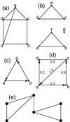 |
Fig. 1. Exemplary graphs. (a) An undirected, connected planar graph – the edge ae can be drawn to the left of vertex d, so that it will not intersect with the edge cd. Edges need not be straight lines. (b) A disconnected graph. Degree-zero vertices, such as g here, are allowed. (c) A directed graph. A path from, e.g., b to c is allowed, but to go back one needs to travel from c → a → b. (d) A mixed weighted graph. (e) The dashed edge is a bridge. After removing this edge, the graph becomes disconnected, so it yields λ(G) = 1. |
Let u and v be adjacent vertices, so e = uv is an edge. It is undirected if one can travel directly from u to v and vice versa. It is directed if only one direction is allowed (Fig. 1c). An undirected graph is one with all of its edges being undirected. Similarly, a directed graph has all of its edges directed. A mixed graph has both directed and undirected edges. A weighted graph has some weights associated to its edges regardless of whether they are directed or undirected (Fig. 1d).
If a connected graph can be disconnected by removing some particular n edges, but not any n − 1 edges, its edge connectivity is λ(G) = n. In particular, if a graph contains a single edge whose removal disconnects the graph, this edge is called a bridge (Fig. 1e). Likewise, a graph’s vertex connectivity κ(G) is the minimal number of vertices whose removal results in a disconnected graph.
For an undirected graph, the handshaking theorem holds:
where |E| is the total number of edges. A graph can be summarised by its adjacency matrix A, whose elements are Aij = 1 if vertices i and j are connected by an edge, and Aij = 0 otherwise. For instance, for the graph in Fig. 1a,
where A12 = 1 means that vertices a and b are joined by an edge, but since A13 = 0 there is no edge between a and c, and so on. For a simple graph, the diagonal is always composed of zeros since there are no loops. It follows that
A degree vector d has elements di ≡ deg(i) = ∑jAij, and the diagonal degree matrix D is defined by Dii = di.
4. Methods
In graph-based clustering methods (Fortunato 2010), the aim is to construct a graph from multivariate data, and then partition that graph into disconnected components (communities) according to some predefined rules and objectives. The components are then associated with different clusters. A vast collection of algorithms has been gathered2. Some detect a predetermined number of communities, whereas others aim to provide the means necessary to decide both the number of clusters and the best partition. A few of the latest approaches are described in the following sections, and then applied to GRB data sets from Sect. 2.
4.1. Continuous k-nearest neighbour
The central concept of several algorithms is the k-nearest neighbour graph (kNN). For every point in the sample, one seeks its k nearest neighbours (commonly employing a Euclidean distance measure) and connects it to them. Such an approach allows one to capture local densities, but it is often sensitive to the value of k. A way of circumventing this issue is the continuous kNN graph (CkNN; Berry & Sauer 2019). Let the (metric) distance between points i and j be denoted by d(i, j), and the distance from i to its k-th nearest neighbour be denoted by dk(i). Then, i and j are joined by an edge if  , where δ is a parameter controlling the sparsity of the graph.
Markov stability is used to assess the relevant partition (Liu & Barahona 2020). Let us consider a Markov process3 on a graph, with a one-step transition matrix M = D−1A. Its stationary distribution is π = dT/(2|E|), and its autocovariance matrix is B(t) = D/(2|E|)P(t)−πTπ, where the transition matrix P(t) = exp[−t(I−M)], with I being the identity matrix.
Thence, the Markov stability r(t, gs) of a partition of the nodes g into c non-overlapping subsets gs is defined as
A good partition is one that attains high values of the Markov stability as a function of t,
achieved for some partition g*. The so-called Markov time t is a parameter that controls the resolution of partitions. For small t, many communities are expected to emerge as local structures in the graph dominate. For larger t, the global features become prominent. Asymptotically, the Markov stability settles on a bipartition. A robust partition persists for long Markov times (i.e. the obtained number of communities is constant), and the dissimilarity of partitions for different t and t′ is low (i.e. the group membership of the nodes does not change rapidly). To measure the latter, the variation of information (VI; Meila 2007) was employed, and the matrix VI(t, t′) contains large blocks with small values.
The VI is based on the concepts of entropy and information. Let us consider a partition 𝒞 of n points into K mutually disjoint clusters 𝒞i. Let ni > 0 be the number of points in cluster 𝒞i. Similarly, let 𝒞′ be another partition into K′ clusters (not necessarily equal to K), and  be the size of cluster
  . The probability that a randomly picked point is in cluster 𝒞i, given the partition 𝒞, is P(i) = ni/n. Similarly, one defines P′(i′). Thence, the entropy associated to the partition 𝒞 is
and similarly for 𝒞′. The entropy is zero only if there is just one cluster in a partition. Let us set  to denote the joint probability that a randomly picked point belongs to clusters 𝒞i and
  in the respective partitions. The mutual information between the two partitions is then defined to be
and ℐ(𝒞,𝒞′) = ℐ(𝒞′,𝒞). Finally, the VI is defined as
where ℋ(.|.) is the conditional entropy. Furthermore, VI is a metric and is bounded to the closed interval [0,log n].
To summarise the whole clustering algorithm, one must first construct a CkNN graph, then partition it. Next, one must choose the partition that has (i) a long plateau in the number of communities against Markov time t and (ii) a low VI of the partitions within it. This implies that the partition is robust. A MATLAB implementation is provided by the authors4.
4.2. CutPC
The CutPC algorithm (Li et al. 2020) starts by constructing a variant of the kNN graph, that is, the natural neighbour (NaN) graph (NNG; Huang et al. 2016). Two vertices u and v are considered to be NaNs if u is a neighbour of v and vice versa. For example, if one were to consider the three points 1, 3, and 4 on a real line, the nearest neighbour of 1 is 3, but the nearest neighbour of 3 is 4, hence 1 and 3 are not NaNs; however, 3 and 4 are NaNs. The definition is natural since it comes from objective reality: one should consider a friend as a person who also thinks of him or her as a friend. In general, two points are associated with each other (i.e., joined by an edge in the NNG) if they are both similar to each other (homophily). The construction of NNG requires tuning no parameters, contrary to the kNN graph, in which the number k of nearest neighbours needs to be set.
Points in sparser regions have fewer NaNs than points in denser regions, which naturally leads one to consider points in very sparse regions as outliers, or noise-induced. These can be identified with the reverse density. First, let us compute the mean NaN distance of point i:
where d(i, j) is the Euclidean distance between i and j, and the sum runs over the j that are NaNs of i. The reverse density is
where the triangular brackets denote the mean over all points in a data set, and α is a tuning parameter (the only free parameter in this algorithm). A point i is considered an outlier if τ(i) > θ, that is, if its mean distance to NaNs exceeds α standard deviations from the mean. After discarding outliers and the edges connected to them from the NNG, the remaining points were divided into connected clusters. Inherently, the clusters are expected to be located around points with high density, and in principle the method should work on overlapping clusters, too, after tweaking the value of α. The algorithm is relatively fast, with complexity of 𝒪(n log n). A MATLAB implementation is provided by the authors5.
4.3. Graph connectivity
A connectivity-based approach to clustering (Li et al. 2019) that takes cluster overlaps into account starts by constructing a kNN graph, Gk. As a rule of thumb, k ≥ 6(m − 1), where m is the dimensionality of the data. The central point of the methodology is to identify a set S of singular points, whose removal will split the graph into clusters. Let us define a set of distance d vertices:

where dGk(u, v) is the path length between vertices u and v. Let us define a new graph,  , where a ≤ 2d, and the edges

Graph  can be connected or disconnected, hence it is composed of one or more components, 𝒞; their number is denoted by
  . The singular index SI of vertex v can then be approximated by the number of these components:
where the sum is over all i such that  . A vertex v is a singular point if SI(v|k, d, a) > 1, meaning there exists more than one cluster in distance d from v. Let us denote the graph that results from removing all singular points by G−S = (V \ S, E). The components of G−S constitute the final clusters. A smaller value of d leads to fewer singular points. A rule of thumb for its choice is 5 ≤ d ≤ diam(Gk), where the diameter diam(Gk) of the graph Gk is the maximum separation of its vertices. The membership of each singular point s may be assigned based on the membership of vertices in the neighbourhood of s. In particular, for each s the path length to the solid clusters was computed, and its membership was assigned to the nearest cluster. In case of a tie, membership was assigned randomly. A MATHEMATICA implementation is available6.
The choice of (d, a) was determined by a grid search for all possibilities. First, the range of d was restricted to d ≤ ⌈diam(Gk)/2⌉ since for larger d the set Vv(d) extends over most of the data, and the resulting partitions contain just one cluster. Therefore, the scan was performed over 5 ≤ d ≤ ⌈diam(Gk)/2⌉, a ≤ 2d. For each d, the VI between a and a − 1 was computed and plotted against the associated a. For all data sets that were examined, most of the range of a resulted in only two clusters and exhibited a long plateau in the values of VI. Among them, the minimal value was chosen, and the associated a was recorded. For every d an a was therefore retrieved. The VI was once again investigated, this time against d, whose value was chosen as the one with minimal VI. The obtained (d, a) were then chosen as parameters for the final clustering.
4.4. fastdp
The method of fast density peaks (fastdp; Sieranoja & Fränti 2019) also utilises the kNN graph. Its key concept is to identify cluster centres as regions with high local density ρ and to be surrounded by more sparsely distributed points. The density at point i is defined as the inverse of the mean distance from i to other vertices of the kNN graph. The cluster centres should also be sufficiently separated from each other. The distance from point i to the nearest point with a higher density is denoted by δ; the latter is named a big brother (BB) of i. The number of clusters K is a user-provided input parameter. Its choice can be made based on the decision plot of (ρ, δ): high values of γ ≡ ρδ are likely to signalise clusters (Rodriguez & Laio 2014). What constitutes a high value is a matter of context, though. The clusters are formed around K points (density peaks) with the highest γ values. The membership of the remaining points is assigned based on their BBs. The algorithm has a very fast and efficient C implementation provided by the authors7.
5. Results
5.1. Continuous k-nearest neighbour
The CkNN algorithm was applied with k = 8 and δ = 2.4, as recommended by Liu & Barahona (2020), for Markov times t ≤ 103, after which a saturation at two clusters was encountered. Two representative results are shown in Fig. 2. In case of BATSE, the number of communities exhibits a prolonged plateau for K = 3, during which the VI drops to zero. This stage is followed by a prominent block corresponding to K = 2. On the other hand, when Suzaku GRBs are considered, there is not much evidence for K > 2, and hence only two clusters are detected. This suggests three communities for BATSE GRBs, and two for the Suzaku ones.
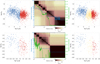 |
Fig. 2. BATSE (upper row) and Suzaku (bottom row) GRBs clustered with the CkNN algorithm. Left and right columns: partitioning into two and three groups, respectively; different colours (symbols – circles, squares, and diamonds) symbolise communities. The middle column shows the evolution of the number of communities and VI with Markov time t. The matrix plot in the background displays the VI(t, t′) matrix. Large blocks with small values on the diagonal relate to the number of communities (depicted with the blue line) that is dependent on the Markov time t. The sizes of the matrix blocks indicate the persistence of the corresponding number of communities. The VI is depicted with the green line. Overall, a significant partition is characterised by a large block of small values of the VI(t, t′) matrix, and a low level of the VI. |
The pictures painted by the remaining four data sets (Fermi, Konus, Swift, and RHESSI) reveal a gradual transition of the domination of two over three groups, with the cases of Fermi and Konus resembling the results for BATSE, while Swift and RHESSI are more similar to Suzaku. This seems to be an effect of the sample size (Tarnopolski 2019a), that is, in less numerous data sets there are simply not enough points to highlight more than two groups. Overall, the results point at either two or three clusters, hence do not conform with the works that find more GRB classes, for example five or seven (Acuner & Ryde 2018; Ruffini et al. 2018).
5.2. CutPC
The CutPC algorithm contains only one free parameter, the tuning coefficient α. While the authors (Li et al. 2020) note that α = 1 should be suitable for most data sets, they observed that sometimes a better clustering is obtained when α is different. Therefore, for the considered GRB samples, the range α ∈ [0, 2] was swept with a step Δα = 0.01. One seeks a stable partitioning, that is, a wide plateau of the number of communities in dependence on α. Two very stable communities are observed for Suzaku, two or three communities for RHESSI (both partitions are very stable; the division into three groups is consistent with Gaussian mixture modelling done by Řípa et al. 2009), and formally four communities for Konus (but see further comments). Fermi and BATSE were inconclusive, that is, partitioning into more than one group does not yield stable clusters. This might be due to severe overlaps of the groups. The Swift data suffer from very non-uniform density of points: the long GRBs are confidently identified, but the short ones are either not classified as a cluster at all, or are randomly divided into several small classes.
Furthermore, for example, in the case of Konus GRBs, clustering into four classes seems erroneous, as two big groups, easily attributed to short and long GRBs, are obtained, in addition to two small ones that contain only a few points each. Overall, many more points are classified by the algorithm as outliers than members of these groups. In Fig. 3 the dependence on α and the two partitions of Konus data are displayed. Figure 4 in turn demonstrates the final graph for α = 1. It is clear from this plot that there are two clusters, which are however connected by a bridge that leads to only one group, which is separated when α is slightly decreased to α = 0.97, leading to the two-group partitioning from Fig. 3c.
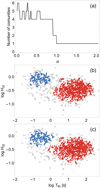 |
Fig. 3. Performance of the CutPC algorithm. (a) Dependence of the number of communities on α for the Konus data; and (b) clustering with α = 0.70 and (c) α = 0.97. Open black points are outliers, and the communities are denoted with different colours (symbols – circles, squares, diamonds, and crosses). |
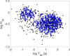 |
Fig. 4. Graph bridge that results with the CutPC algorithm applied to Konus data when α = 1 was employed, formally leading to only one cluster. |
All in all, a two-group classification is easily visible, but there is no evidence to either support or reject the presence of more groups. The algorithm performs poorly on data with large variations in density, which is the case of GRB data. However, its future development aims to circumvent this problem (Li et al. 2020).
5.3. Graph connectivity
The connectivity-based method was employed with k = 6 for all data sets. For Suzaku, RHESSI, Swift, and Konus, a stable partitioning was obtained for two clusters. They are consistent with both mixture modelling and other graph-based methods. In the case of Fermi and BATSE, however, the results are uninformative, that is, no plateau in VI was reached before the number of communities dropped to one. A two-group partition of Swift GRBs is shown in Fig. 5.
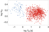 |
Fig. 5. Clusters in Swift GRBs identified by the connectivity method. Communities are marked with different colours (symbols – circles and squares). Open symbols denote singular points, assigned to clusters based on proximity. |
5.4. fastdp
The fastdp algorithm was run for various values of k. For 2 ≤ k < 10, the partitions were very unstable, and they settled for k ≥ 10. Eventually, k = 30 was utilised for all data sets.
For BATSE, the γ values indicate two classes (Fig. 6). However, there are several values clearly above the bulk around zero, but they are significantly lower than the two highest ones. A much less clear picture is obtained for Fermi, for which the γ plot hints at about 15 classes, which seems highly unreliable and hence inconclusive. For Konus, it appears that clustering into three groups is appropriate; however, the division seems non-standard, yet similar to what was obtained with the Gaussian mixture model in the case of Fermi GRBs (Tarnopolski 2019b). Swift’s clustering into two groups is clearly erratic since the separation between short and long GRBs occurs at T90 ≲ 100 s. Partitioning into three classes is more sensible; however, it is unclear why the long GRBs ought to be divided also at T90 ≲ 100 s. It appears the algorithm just divides the cluster at the point of the highest local density into groups lying to the left and right of it. Finally, RHESSI and Suzaku are confidently divided into two standard groups, with only vague hints of a third one – in such a case, the long class is cut into approximately equal halves.
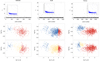 |
Fig. 6. Clusters identified in RHESSI (left column), Swift (middle column), and Konus GRBs (right column) with fastdp. Upper row: decision plots; the insets are the (ρ, δ) planes, with a few contours γ ≡ ρδ = const. displayed. Middle and bottom rows: resulting partitions into two and three clusters, respectively, with different colours (symbols – circles, squares, and diamonds) denoting the communities. |
6. Discussion
The objective of any clustering scheme is to divide a data set into groups within which points are most similar to each other as per some metric. There are various principles and heuristics for achieving this goal. In graph-based methods utilised herein, clusters were retrieved based on variants of the kNN graphs constructed from the samples at hand. These methods exploit not just the local densities, as the Gaussian mixture models do, but they explore the network relations (neighbours, big brothers, etc.) between pairs and subgroups of points, and how the structure of the graphs built from the samples (kNN graphs and its variants) depends on free parameters of the algorithms, seeking a robust, stable partition into communities (see Sect. 4). Graph-based algorithms can be hierarchical in nature, or can rely on distances between points or local densities (in the network sense) that signify centres of clusters. Usually they work well on groups sufficiently separated, but when overlaps become substantial – as in case of GRBs – the results become less unambiguous. The overlaps in the data seem to be the most serious source of biases. One needs to bear in mind there are also instrumental biases; for example, Swift is more sensitive in soft bands than BATSE was, therefore it yields a much lower fraction of short GRBs than other data sets. Hence the parallel investigation of six GRB samples was conducted herein to paint a more complete picture. For discussions on the instrumental effects and biases, readers can refer to Shahmoradi (2013), Shahmoradi & Nemiroff (2015), Řípa & Mészáros (2016), Tarnopolski (2019b) and the references therein.
Some of the employed graph-based methods applied to GRBs worked relatively well for some data sets, while they gave rather unreliable results for others. Also, different algorithms gave different results for the same samples. It is thence worth emphasising that the mathematically formulated goals to be achieved by a particular algorithm can be apparently counter intuitive, especially when the desired outcome is not unequivocal. However, there are two significant outcomes to point out. The first one being that smaller samples (e.g., Suzaku) rather confidently exhibit two GRB classes, while bigger ones (e.g., BATSE) do not rule out the possibility of three being present. This observation that bigger samples are more liberal when it comes to accepting the possibility of a third class was also observed when using mixture models (Tarnopolski 2019a). The second major result is that there are no hints of more than three groups (despite some works implying even five or seven).
Finally, a more robust classification could be achieved by combining the heuristics of different approaches, for example, weighted kNN graphs are likely to lead to better results. The weights, in turn, could be inferred from other GRB properties, not necessarily stemming from the metric relations of the considered parameter spaces. One should also note that all of the described algorithms can in principle operate on an arbitrary number of parameters, hence they do not need to be restricted to two-dimensional duration-hardness ratio spaces. This is a direction worth exploring in a subsequent work.
7. Summary
The obtained GRB clusterings generally agree that there are two groups that can be associated with the conventional short–long dichotomy. In many cases, though, rejecting the possibility of a third group cannot be immediately discarded. In such cases, the resulting partitions split the long group in two parts that are roughly consistent with the intermediate and long GRB types. In summary, (i) it is therefore still unclear whether there are two or three distinct classes, but (ii) the graph-based methods led to no indications of, for example, five or seven groups, and (iii) after further development, such methods are promising tools for looking at GRBs from a different perspective, and they can prove to be useful in classifying other astronomical objects, such as stars or galaxies as well.
A Markov process is a stochastic model in which the probability of each event (the transition between states) depends only on the state of the previous event.
Acknowledgments
The author acknowledges support by the Polish National Science Centre through the OPUS grant No. 2017/25/B/ST9/01208.
References
- Acuner, Z., & Ryde, F. 2018, MNRAS, 475, 1708 [NASA ADS] [CrossRef] [Google Scholar]
- Ahumada, T., Singer, L. P., Anand, S., et al. 2021, Nat. Astron., 5, 917 [NASA ADS] [CrossRef] [Google Scholar]
- Balastegui, A., Ruiz-Lapuente, P., & Canal, R. 2001, MNRAS, 328, 283 [NASA ADS] [CrossRef] [Google Scholar]
- Berry, T., & Sauer, T. 2019, Found. Data Sci., 1, 1 [Google Scholar]
- Bonnaire, T., Aghanim, N., Decelle, A., & Douspis, M. 2020, A&A, 637, A18 [NASA ADS] [CrossRef] [EDP Sciences] [Google Scholar]
- Bromberg, O., Nakar, E., Piran, T., & Sari, R. 2013, ApJ, 764, 179 [NASA ADS] [CrossRef] [Google Scholar]
- Campana, R., Massaro, E., Gasparrini, D., Cutini, S., & Tramacere, A. 2008, MNRAS, 383, 1166 [Google Scholar]
- Chattopadhyay, S., & Maitra, R. 2017, MNRAS, 469, 3374 [NASA ADS] [CrossRef] [Google Scholar]
- Chattopadhyay, S., & Maitra, R. 2018, MNRAS, 481, 3196 [NASA ADS] [Google Scholar]
- Chattopadhyay, T., Misra, R., Chattopadhyay, A. K., & Naskar, M. 2007, ApJ, 667, 1017 [NASA ADS] [CrossRef] [Google Scholar]
- Farrah, D., Connolly, B., Connolly, N., et al. 2009, ApJ, 700, 395 [NASA ADS] [CrossRef] [Google Scholar]
- Fortunato, S. 2010, Phys. Rep., 486, 75 [NASA ADS] [CrossRef] [Google Scholar]
- Hakkila, J., Haglin, D. J., Pendleton, G. N., et al. 2000, ApJ, 538, 165 [NASA ADS] [CrossRef] [Google Scholar]
- Hakkila, J., Giblin, T. W., Roiger, R. J., et al. 2003, ApJ, 582, 320 [NASA ADS] [CrossRef] [Google Scholar]
- Hakkila, J., Giblin, T. W., Roiger, R. J., et al. 2004, Baltic Astron., 13, 211 [NASA ADS] [Google Scholar]
- Horváth, I. 1998, ApJ, 508, 757 [CrossRef] [Google Scholar]
- Horváth, I. 2002, A&A, 392, 791 [NASA ADS] [CrossRef] [EDP Sciences] [Google Scholar]
- Horváth, I., Balázs, L. G., Bagoly, Z., Ryde, F., & Mészáros, A. 2006, A&A, 447, 23 [NASA ADS] [CrossRef] [EDP Sciences] [Google Scholar]
- Horváth, I., Balázs, L. G., Bagoly, Z., & Veres, P. 2008, A&A, 489, L1 [NASA ADS] [CrossRef] [EDP Sciences] [Google Scholar]
- Horváth, I., Bagoly, Z., Balázs, L. G., et al. 2010, ApJ, 713, 552 [CrossRef] [Google Scholar]
- Horváth, I., Tóth, B. G., Hakkila, J., et al. 2018, Ap&SS, 363, 53 [CrossRef] [Google Scholar]
- Horváth, I., Hakkila, J., Bagoly, Z., et al. 2019, Ap&SS, 364, 105 [CrossRef] [Google Scholar]
- Huang, J., Zhu, Q., Yang, L., & Feng, J. 2016, Knowledge-Based Syst., 92, 71 [Google Scholar]
- Huja, D., Mészáros, A., & Řípa, J. 2009, A&A, 504, 67 [NASA ADS] [CrossRef] [EDP Sciences] [Google Scholar]
- Jespersen, C. K., Severin, J. B., Steinhardt, C. L., et al. 2020, ApJ, 896, L20 [NASA ADS] [CrossRef] [Google Scholar]
- Klebesadel, R. W., Strong, I. B., & Olson, R. A. 1973, ApJ, 182, L85 [NASA ADS] [CrossRef] [Google Scholar]
- Koen, C., & Bere, A. 2012, MNRAS, 420, 405 [NASA ADS] [CrossRef] [Google Scholar]
- Kohonen, T. 1982, Biol. Cybern., 43, 59 [Google Scholar]
- Kouveliotou, C., Meegan, C. A., Fishman, G. J., et al. 1993, ApJ, 413, L101 [NASA ADS] [CrossRef] [Google Scholar]
- Kwong, H. S., & Nadarajah, S. 2018, MNRAS, 473, 625 [NASA ADS] [CrossRef] [Google Scholar]
- Li, Y.-F., Lu, L.-H., & Hung, Y.-C. 2019, in Intelligent Computing, eds. K. Arai, S. Kapoor, & R. Bhatia (Cham: Springer International Publishing), 442 [Google Scholar]
- Li, L.-T., Xiong, Z.-Y., Dai, Q.-Z., et al. 2020, Inf. Syst., 91, 101504 [CrossRef] [Google Scholar]
- Lien, A., Sakamoto, T., Barthelmy, S. D., et al. 2016, ApJ, 829, 7 [Google Scholar]
- Liu, Z., & Barahona, M. 2020, Appl. Netw. Sci., 5, 1 [NASA ADS] [CrossRef] [Google Scholar]
- Maritz, J., Maritz, E., & Meintjes, P. 2017, The Proceedings of SAIP2016, the 61st Annual Conference of the South African Institute of Physics, Dr. Steve Peterson and Dr. Sahal Yacoob (UCT/2016), 243 [Google Scholar]
- Meila, M. 2007, J. Multivariate Anal., 98, 873 [CrossRef] [Google Scholar]
- Modak, S., Chattopadhyay, A. K., & Chattopadhyay, T. 2018, Commun. Stat. - Simul. Comput., 47, 1088 [Google Scholar]
- Mukherjee, S., Feigelson, E. D., Jogesh Babu, G., et al. 1998, ApJ, 508, 314 [NASA ADS] [CrossRef] [Google Scholar]
- Narayana Bhat, P., Meegan, C. A., von Kienlin, A., et al. 2016, ApJS, 223, 28 [NASA ADS] [CrossRef] [Google Scholar]
- Ohmori, N., Yamaoka, K., Ohno, M., et al. 2016, PASJ, 68, S30 [NASA ADS] [CrossRef] [Google Scholar]
- Rajaniemi, H. J., & Mähönen, P. 2002, ApJ, 566, 202 [NASA ADS] [CrossRef] [Google Scholar]
- Rodriguez, A., & Laio, A. 2014, Science, 344, 1492 [NASA ADS] [CrossRef] [Google Scholar]
- Roiger, R. J., Hakkila, J., Haglin, D. J., Pendleton, G. N., & Mallozzi, R. S. 2000, in Gamma-ray Bursts, 5th Huntsville Symposium, eds. R. M. Kippen, R. S. Mallozzi, & G. J. Fishman, Am. Inst. Phys. Conf. Ser., 526, 38 [NASA ADS] [CrossRef] [Google Scholar]
- Ruffini, R., Wang, Y., Aimuratov, Y., et al. 2018, ApJ, 852, 53 [Google Scholar]
- Shahmoradi, A. 2013, ApJ, 766, 111 [NASA ADS] [CrossRef] [Google Scholar]
- Shahmoradi, A., & Nemiroff, R. J. 2015, MNRAS, 451, 126 [NASA ADS] [CrossRef] [Google Scholar]
- Sieranoja, S., & Fränti, P. 2019, Pattern Recog. Lett., 128, 551 [Google Scholar]
- Svinkin, D. S., Frederiks, D. D., Aptekar, R. L., et al. 2016, ApJS, 224, 10 [CrossRef] [Google Scholar]
- Tarnopolski, M. 2015a, Ap&SS, 359, 20 [NASA ADS] [CrossRef] [Google Scholar]
- Tarnopolski, M. 2015b, A&A, 581, A29 [NASA ADS] [CrossRef] [EDP Sciences] [Google Scholar]
- Tarnopolski, M. 2016a, MNRAS, 458, 2024 [NASA ADS] [CrossRef] [Google Scholar]
- Tarnopolski, M. 2016b, Ap&SS, 361, 125 [CrossRef] [Google Scholar]
- Tarnopolski, M. 2019a, J. Ital. Astron. Soc., 1, 45 [NASA ADS] [Google Scholar]
- Tarnopolski, M. 2019b, ApJ, 870, 105 [CrossRef] [Google Scholar]
- Tarnopolski, M. 2019c, ApJ, 887, 97 [NASA ADS] [CrossRef] [Google Scholar]
- Tarnopolski, M. 2020, ApJ, 897, 77 [NASA ADS] [CrossRef] [Google Scholar]
- Tóth, B. G., Rácz, I. I., & Horváth, I. 2019, MNRAS, 486, 4823 [CrossRef] [Google Scholar]
- Tramacere, A., & Vecchio, C. 2013, A&A, 549, A138 [NASA ADS] [CrossRef] [EDP Sciences] [Google Scholar]
- Řípa, J., & Mészáros, A. 2016, Ap&SS, 361, 370 [CrossRef] [Google Scholar]
- Řípa, J., Mészáros, A., Wigger, C., et al. 2009, A&A, 498, 399 [NASA ADS] [CrossRef] [EDP Sciences] [Google Scholar]
- Řípa, J., Mészáros, A., Veres, P., & Park, I. H. 2012, ApJ, 756, 44 [CrossRef] [Google Scholar]
- Veres, P., Bagoly, Z., Horváth, I., Mészáros, A., & Balázs, L. G. 2010, ApJ, 725, 1955 [NASA ADS] [CrossRef] [Google Scholar]
- von Kienlin, A., Meegan, C. A., Paciesas, W. S., et al. 2020, ApJ, 893, 46 [Google Scholar]
- Wilson, R. J. 1998, Introduction to Graph Theory (London: Addison Wesley Longman Limited) [Google Scholar]
- Yang, E. B., Zhang, Z. B., & Jiang, X. X. 2016, Ap&SS, 361, 257 [NASA ADS] [CrossRef] [Google Scholar]
- Zhang, Z.-B., & Choi, C.-S. 2008, A&A, 484, 293 [NASA ADS] [CrossRef] [EDP Sciences] [Google Scholar]
- Zhang, Z.-B., Yang, E.-B., Choi, C.-S., & Chang, H.-Y. 2016, MNRAS, 462, 3243 [NASA ADS] [CrossRef] [Google Scholar]
All Figures
|
Fig. 1. Exemplary graphs. (a) An undirected, connected planar graph – the edge ae can be drawn to the left of vertex d, so that it will not intersect with the edge cd. Edges need not be straight lines. (b) A disconnected graph. Degree-zero vertices, such as g here, are allowed. (c) A directed graph. A path from, e.g., b to c is allowed, but to go back one needs to travel from c → a → b. (d) A mixed weighted graph. (e) The dashed edge is a bridge. After removing this edge, the graph becomes disconnected, so it yields λ(G) = 1. |
| In the text | |
|
Fig. 2. BATSE (upper row) and Suzaku (bottom row) GRBs clustered with the CkNN algorithm. Left and right columns: partitioning into two and three groups, respectively; different colours (symbols – circles, squares, and diamonds) symbolise communities. The middle column shows the evolution of the number of communities and VI with Markov time t. The matrix plot in the background displays the VI(t, t′) matrix. Large blocks with small values on the diagonal relate to the number of communities (depicted with the blue line) that is dependent on the Markov time t. The sizes of the matrix blocks indicate the persistence of the corresponding number of communities. The VI is depicted with the green line. Overall, a significant partition is characterised by a large block of small values of the VI(t, t′) matrix, and a low level of the VI. |
| In the text | |
|
Fig. 3. Performance of the CutPC algorithm. (a) Dependence of the number of communities on α for the Konus data; and (b) clustering with α = 0.70 and (c) α = 0.97. Open black points are outliers, and the communities are denoted with different colours (symbols – circles, squares, diamonds, and crosses). |
| In the text | |
|
Fig. 4. Graph bridge that results with the CutPC algorithm applied to Konus data when α = 1 was employed, formally leading to only one cluster. |
| In the text | |
|
Fig. 5. Clusters in Swift GRBs identified by the connectivity method. Communities are marked with different colours (symbols – circles and squares). Open symbols denote singular points, assigned to clusters based on proximity. |
| In the text | |
|
Fig. 6. Clusters identified in RHESSI (left column), Swift (middle column), and Konus GRBs (right column) with fastdp. Upper row: decision plots; the insets are the (ρ, δ) planes, with a few contours γ ≡ ρδ = const. displayed. Middle and bottom rows: resulting partitions into two and three clusters, respectively, with different colours (symbols – circles, squares, and diamonds) denoting the communities. |
| In the text | |
Current usage metrics show cumulative count of Article Views (full-text article views including HTML views, PDF and ePub downloads, according to the available data) and Abstracts Views on Vision4Press platform.
Data correspond to usage on the plateform after 2015. The current usage metrics is available 48-96 hours after online publication and is updated daily on week days.
Initial download of the metrics may take a while.