| Issue |
A&A
Volume 656, December 2021
|
|
|---|---|---|
| Article Number | A138 | |
| Number of page(s) | 16 | |
| Section | Interstellar and circumstellar matter | |
| DOI | https://doi.org/10.1051/0004-6361/202141686 | |
| Published online | 15 December 2021 | |
PENELLOPE
II. CVSO 104: A pre-main sequence close binary with an optical companion in Ori OB1★
1
INAF – Osservatorio Astrofisico di Catania,
via S. Sofia 78,
95123
Catania,
Italy
e-mail: This email address is being protected from spambots. You need JavaScript enabled to view it.
2
European Southern Observatory,
Karl-Schwarzschild-Strasse 2,
85748
Garching bei München,
Germany
3
INAF – Osservatorio Astronomico di Capodimonte,
via Moiariello, 16,
80131
Napoli,
Italy
4
Konkoly Observatory, Research Centre for Astronomy and Earth Sciences, Eötvös Loránd Research Network (ELKH),
Konkoly-Thege Miklós út 15-17,
1121
Budapest,
Hungary
5
ELTE Eötvös Loránd University, Institute of Physics,
Pázmány Péter sétány 1/A,
1117
Budapest,
Hungary
6
Purple Mountain Observatory, Chinese Academy of Sciences,
10 Yuanhua Road,
Nanjing
210023,
PR China
7
INAF – Osservatorio Astronomico di Roma,
via di Frascati 33,
00078
Monte Porzio Catone,
Italy
8
Kavli Institute for Astronomy and Astrophysics, Peking University,
Yiheyuan 5,
Haidian Qu,
100871
Beijing,
PR China
9
Max Planck Institute for Astronomy,
Königstuhl 17,
69117
Heidelberg,
Germany
10
SETI Institute,
189 Bernardo Ave, Suite 200,
Mountain View,
CA
94043,
USA
11
Stony Brook University,
Stony Brook,
NY
11794,
USA
12
Crimean Astrophysical Observatory,
298409
Nauchny,
Crimea
13
Univ. Grenoble Alpes, CNRS, IPAG,
38000
Grenoble,
France
14
Observatoire de Paris, PSL University, Sorbonne Université, CNRS, LERMA,
75014
Paris,
France
Received:
30
June
2021
Accepted:
11
September
2021
Abstract
We present the results of our study of the close pre-main sequence spectroscopic binary CVSO 104 in Ori OB1, based on data obtained within the PENELLOPE legacy program. We derive, for the first time, the orbital elements of the system and the stellar parameters of the two components. The system is composed of two early M-type stars and has an orbital period of about five days and a mass ratio of 0.92, but contrary to expectations, it does not appear to have a tertiary companion. Both components have been (quasi-)synchronized, but the orbit is still very eccentric. The spectral energy distribution clearly displays a significant infrared excess that is compatible with a circumbinary disk. The analysis of He I and Balmer line profiles, after the removal of the composite photospheric spectrum, reveals that both components are accreting at a similar level. We also observe excess emission in Hα and Hβ, which appears redshifted or blueshifted by more than 100 km s−1 with respect to the mass center of the system, depending on the orbital phase. This additional emission could be connected with accretion structures, such as funnels of matter from the circumbinary disk. We also analyze the optical companion located at about 2.″4 from the spectroscopic binary. This companion, which we named CVSO 104 B, turns out to be a background Sun-like star that is not physically associated with the PMS system and does not belong to Ori OB1.
Key words: stars: pre-main sequence / binaries: spectroscopic / stars: low-mass / accretion, accretion disks / protoplanetary disks / stars: individual: CVSO104
Based on data obtained within ESO programme 106.20Z8.
© ESO 2021
1 Introduction
The formation of stars and planets is strongly influenced by the conditions in their environment (circumstellar disks, jets, and winds) during their early life. The majority of stars are formed in binary and multiple systems, which, for sufficiently small separations, allows for information on their components to be obtained, such as dynamical masses. It is therefore very important to detect and study young pre-main sequence (PMS) close binaries for deriving their orbital and stellar properties and to understand how the binarity affects the planet formation. Moreover, well-characterized early-PMS binary systems are critical in constraining theoretical evolutionary tracks, which are used to derive fundamental stellar properties, but are often affected by offsets of up to 50% in the predicted masses, as compared to the dynamical mass estimates (e.g., Covino et al. 2004; Hillenbrand & White 2004; Stassun et al. 2014). Such PMS binaries are also very important for studying the mass accretion process in a different field geometry from that of single stars. Both the observations and numerical simulations show that quasi-periodic bursts of accretion are expected in close binaries, with a different pattern for circular and eccentric systems (e.g., Muñoz & Lai 2016; Gillen et al. 2017). For eccentric systems, the accretion bursts, originating from the impact of nearly free-falling matter on the high atmospheric layers of each of the two components, are more frequently observed near the periastron passages (e.g., Kóspál et al. 2018; Tofflemire et al. 2019). The simulations also show gas streams from the circumbinary disk flowing to each component through the L2 and L3 Lagrangian points (e.g., de Val-Borro et al. 2011; Muñoz & Lai 2016).
We present here the spectroscopic orbit of CVSO 104 (Haro 5-64), which is a classical T Tauri star located in the ~ 5 Myr old Orion OB1b association. It was discovered as a star with Hα emission in the region of the Horsehead Nebula (IC 434) by Haro & Moreno (1953) with objective-prism observations. It was detected in the Kiso survey of emission-line objects by Wiramihardja et al. (1989), who confirmed it as a strong Hα emitter. Briceño et al. (2005) observed this star as part of the CIDA Variability Survey of Orion OB1 (CVSO) and reported it as a variable source with Hα and Li I λ6708 equivalent widths of −62.90Å and 0.30 Å, respectively. The spectra analyzed in the present paper have been obtained as part of the PENELLOPE program running at the Very Large Telescope (VLT), a ground-based follow-up large program (see Manara et al. 2021, hereafter Paper I) of the ULLYSES HST program1 (Roman-Duval et al. 2020).
The Gaia EDR3 release lists a parallax ϖ = 2.73 ± 0.03 mas for the object, putting it at a distance of 366 ± 4 pc, that is, within the Orion star forming region. Its magnitude, G = 14.45, is too faint for Gaia to provide radial velocity measurements. Based on a limited set of APOGEE-2 spectra, Kounkel et al. (2019) identified it as a double-lined binary, with a mass ratio of 0.988 ± 0.063. It is thus a perfect target for binarity follow-up studies. As short-period binaries may be induced by the gravitational torque from an additional companion (e.g., Eggleton & Kiseleva-Eggleton 2001; Naoz & Fabrycky 2014), it is also interesting to know if the system is, in fact, triple.
Gaia lists a slightly fainter (ΔG = 0.14) and redder visual companion at a separation of 2.39′′. With a parallax of ϖ = 1.49 ± 0.03 mas, corresponding to a distance of about 670 pc, this optical companion is, however, unrelated to the much closer Ori OB1 (Tokovinin et al. 2020), as also confirmed by the analysis of its spectra presented in Sect. 3.3. From now on, we will refer to this background star as CVSO 104 B, while we will refer to our target as CVSO 104 A.
The paper is organized as follows. Section 2 reports the observations used in this work. The results of the analysis of the data are then described in Sect. 3 and discussed in Sect. 4. We finally summarize our conclusions in Sect. 5.
2 Observations
2.1 Spectroscopy
High-resolution spectroscopy (R ≃ 70 000) was performed with the Ultraviolet and Visual Echelle Spectrograph (UVES, Dekker et al. 2000) within the PENELLOPE Large Program (ESO Prog. ID. 106.20Z8; see Paper I). Three UVES spectra were acquired within two days of the HST observation of CVSO 104 A+B and a fourth one was purposely requested by us a few days later, after the clear detection of the two components in the spectra of this spectroscopic binary. All these spectra were taken with the same position angle of 109 ° for the slit, aligning it with the optical pair. Medium-resolution (R ~ 10 000–20 000) broad-wavelength coverage spectroscopy was obtained using the X-shooter instrument (Vernet et al. 2011). The strategy of spectroscopic observations and details on data reduction are explained in Paper I. Particular attention was paid to the order trace and extraction to separate the spectra of the two stars of the visual pair.
CVSO 104 A+B was also observed during five visits (two in February 2017 and three in October 2017) in the framework of the APOGEE survey (Ahumada et al. 2020), which obtains R ~ 22 500 spectra in the H-band. Since the radial velocities measured on APOGEE spectra and reported in the SDSS Data Release 16 (Jönsson et al. 2020) were derived by assuming the object as a single star, they are not usable. We therefore downloaded the APOGEE spectra2 and derived the velocities of both components, in the same way as we did for the UVES and X-shooter spectra (see Sect. 3.2).
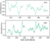 |
Fig. 1 TESS light curves of CVSO 104 A+B in 2018 (top) and 2020 (bottom). |
2.2 Photometry
Space-born accurate photometry was obtained with NASA’s Transiting Exoplanet Survey Satellite (TESS; Ricker et al. 2015). CVSO 104 A+B was observed in sector 6 with 1426s exposure times between 2018-12-15 and 2019-01-06, as well as in sector 32 with 475s exposure times between 2020-11-20 and 2020-12-16; this latter data set is contemporaneous to our spectroscopic observations. Given the pixel size of TESS, the optical companion will contribute to the light curve. We downloaded the data from the MAST archive and created light curves using the LIGHTKURVE3 package by using a mask that contained all the neighboring pixels having S∕N > 6 (see Fig. 1). The 2018 data had a mean flux of 1244 ± 51 e− s−1, while the 2020 data set had a similar mean flux of 1221 ± 58 e− s−1.
To get the color information that is lacking in TESS data and to separate the contribution of the two visual components of the optical pair, several ground-based facilities were involved in the observation of this object during the HST and VST observations. In the present work, we make use of data taken with four different instruments.
We observed CVSO 104 at the M. G. Fracastoro station (Serra La Nave, Mt. Etna, 1750 m a.s.l.) of the Osservatorio Astrofisico di Catania (OACT, Italy) from 25 November to 16 December 2020. We used the facility imaging camera at the 0.91 m telescope with a set of broad-band Bessel filters (B, V, R, I, Z) as well as two narrow-band Hα filters centered on the line core (Hα9) and on the redward continuum (Hα18). The index Hα18 –Hα9 is basically ameasure of intensity of the Hα emission in units of the continuum that can be converted into equivalent width (EW) of Hα (Frasca et al. 2018). Details on photometric observations and data reduction can be found in Paper I. We note that the two visual components are clearly resolved only in the nights with good seeing (see Fig. 2), with the exception of the Z filters in which the image is slightly out of focus. We have therefore extracted the photometry of the stars in the field of CVSO 104 from the calibrated images, using apertures of 5′′ of radius, which include both components of the visual pair. To measure the magnitude difference of the two visual components in the images taken with the best seeing, we used an approach similar to that of Covino et al. (2004).
CVSO 104 was also observed from 6 November to 26 December, 2020 with the 0.8 m RC80 telescope of Konkoly Observatory (Hungary) using Bessel BV and Sloan r′i′ filters. Details about the instrument, data reduction, and photometry are provided in Ábrahám et al. (in prep.). In most of the images, the binary and the visual companion could be properly separated. We performed PSF photometry separately for CVSO 104 A and B in each image. As we show in Sect. 3.1, CVSO 104 B is non-variable, therefore, we calculated its average flux in each filter. Then we added these values to the fluxes of CVSO 104 A, to obtain a full light curve of the visual pair CVSO 104 A+B during the run to be used together with other data sets. To this aim the r′, i′ magnitudes were converted to RC, IC using the prescription given by Lupton (2005)4.
We used BV ri photometry collected by AAVSOnet5, which is a set of robotic telescopes operated by volunteers for the American Association of Variable Star Observers (AAVSO). Stars in the AAVSO Photometric All-Sky Survey (APASS, Henden et al. 2018) were used to calibrate the AAVSO photometric data for our targets. The r, i magnitudes were converted toRC, IC as was donefor the Konkoly photometry. We incorporated data taken by the amateur observers of the AAVSO6, in response to AAVSO Alert Notice 725. Finally, some additional BV RI photometry was obtained at the Crimean Astrophysical Observatory (CrAO) on the AZT-11 1.25 m telescope.
The photometry obtained with the latter instruments includes both components in the aperture. The multiband light curve of CVSO 104 A+B during 30 nights including the ULLYSES and PENELLOPE campaigns is displayed in Fig. A.1.
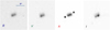 |
Fig. 2 Portion of images acquired at OACT on 16 December 2020 in BV RI bands centered on the visual pair CVSO 104 A+B. North is up and east is to the left and the two components are indicated in the R-band image. We note how the relative brightness of the two stars changes in the different bands, with A becoming brighter than B in the I band. |
3 Results
3.1 Photometry
The TESS light curves (Fig. 1) show rather stochastic variations, albeit quasi-periodic. The period analysis provides different results depending on the epoch of observations and the different techniques. Periodograms reveal that the most likely period for the 2018 data set is 4.73 days, while for the 2020 data, this is 4.91 days, similar to the photometric variability period of 4.68 days in the R-band reported by Karim et al. (2016), as well as to the orbital period we derived (see below). Using the CLEAN deconvolution algorithm (Roberts et al. 1987), we found the maximum power in 2018 at 2.31 days, that is, about the half period of the periodogram and the second highest peak at about 4.53 days. In 2020, the highest peak corresponds to 4.73 days. However, for both data sets, folding the data with any of the above periods does not reveal a convincing phase diagram.
The ground-based multiband light curve (Fig. A.1) shows a stochastic behaviour with at least two bursts fully observed in BV RI bands. The intensity of the bursts is clearly stronger in the bluer bands. However, no intensification of the Hα emission is observed in the OACT photometry contemporaneous to the stronger burst and the variations of Hα EW do not seem to be correlated or anticorrelated with the brightness variations.
While the contribution of CVSO 104 B is included in the photometric data presented in Fig. A.1, our analyses suggest that this source is non-variable or that its variability is negligible in comparison to CVSO 104 A. As a first check, we compared the Gaia EDR3 G-band magnitude uncertainty of component B with the corresponding Gaia magnitude uncertainties of other stars of the same brightness (we used Fig. 5.15 from the Gaia Early Data Release 3 Documentation V1.17 for this comparison). We concluded that the relative flux error of component B, 0.02%, agrees with the representative numbers from similarly bright non-variable stars for which a similar number of observations were taken. We also plotted the light curves of CVSO 104 B, using the spatially resolved photometry obtained at OACT and Konkoly observatories (Sect. 2.2). The plot shown in Fig. A.2 also confirms that the source was constant within the measurement uncertainties, if we neglect very small systematic differences between Konkoly and OACT. In order to check this claim on more quantitative grounds, we calculated the χ2 and the probability P(χ2) that the magnitude variations have a random occurrence (e.g., Press et al. 1992). We found, for the Konkoly dataset, values of P(χ2) of 0.21, 0.22, 0.35, and 0.25 for B, V, RC, and IC bands, respectively, which indicates that these variations are non-significant.
Heliocentric radial velocities of the two components of CVSO 104 A.
3.2 Radial velocity
The radial velocity was measured by cross-correlating the spectra with late-type templates. For the X-shooter spectrum, we selected only the regions with the best S/N in the VIS arm – the one with the highest resolution – and adopted as template a BT-Settl synthetic spectrum (Allard et al. 2012), with [Fe/H] = 0, Teff = 4000 K, and log g = 4.0. For the UVES spectra, we adopted the same template and an HARPS spectrum of GJ 514 (M1V, RV = 14.606 km s−1, Jönsson et al. 2020), obtaining the same results within the errors. This analysis was carried out with the IRAF8 task FXCOR excluding emission lines and very broad features that can blur the peaks of the cross-correlation function (CCF). For a better measure of the centroids and full width at half maximum (FWHM) of the CCF peaks of the two components, we applied a two-Gaussian fit. The RV error, σRV, was computed by FXCOR according to the fitted peak height and the antisymmetric noise as described by Tonry & Davis (1979). We used thesame BT-Settl template to measure RVs in the APOGEE spectra by cross-correlation. The individual values of RV measured inour and APOGEE spectra are listed in Table 1.
We searched for the best orbital period by applying a periodogram analysis (Scargle 1982) and the CLEAN deconvolution algorithm (Roberts et al. 1987) to the RVs of the primary and secondary components. The data folded with the best period (maximum amplitude in the power spectrum) display a smooth variation with an asymmetrical shape, typical for an eccentric RV orbital motion. Then, we fitted the observed RV curve with the CURVEFIT routine (Bevington & Robinson 2003) to determine the orbital parameters and their standard errors. This also allowed us to improve the determination of the orbital period, finding Porb= 5.025 days (see Fig. 3). The orbital parameters are reported in Table 2. We note that the high eccentricity, e ≃ 0.39, is in line with the simulations of Zrake et al. (2021), who show that equal-mass binaries accreting from a circumbinary disk evolve toward an orbital eccentricity of e ~ 0.45, unless they start with a nearly circular orbit (e ≲ 0.08).
In addition, we searched for signatures of an eventual third companion, yet unresolved, in UVES spectra of CVSO 104 A, independently on Gaia. For this purpose, we applied the Broadening Function (BF) method (Rucinski 2012), which is a linear deconvolution operation. Prior to the analysis, all emission lines were carefully removed from the spectra. However, no signatures of a third stellar body were found in the BF profiles. Furthermore, no residual peak at the velocity of the optical companion, CVSO 104 B (RV ≃ 42.9 ± 0.5 km s−1), was found either in the BFs or in the CCFs. This confirms that the extraction of the spectra allowed us to separate A and B components without significant contamination.
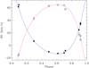 |
Fig. 3 Heliocentric radial velocity curve (circles = UVES, squares = APOGEE, diamonds = X-shooter data) of CVSO 104 A. Filled and open symbols have been used for the primary (more massive) and secondary component, respectively.The blue and red lines represent the orbital solution (Table 2) for the primary and secondary component, respectively. |
Orbital and stellar parameters of CVSO 104 A.
3.3 Stellar parameters
In the PENELLOPE survey, we used the code ROTFIT to determine the atmospheric parameters, v sin i, and veiling for single objects (Frasca et al. 2015, 2017; Paper I). We used this code for determining the parameters of CVSO 104 B and found Teff = 5750 ± 100 K, log g = 4.40 ± 0.12 dex, [Fe/H] = 0.08 ± 0.07 dex, RV = 42.9 ± 0.5 km s−1, and v sin i < 2 km s−1, namely, CVSO 104 B turns out to be a slowly-rotating Sun-like star. Furthermore, there is no lithium λ6708Å absorption line and no chromospheric emission is visible in the Hα line core (see Fig. A.3). Therefore, we do not expect significant brightness variations, compared to CVSO 104 A, from this background star, in agreement with the results from the ground-based photometry (Sect. 3.1).
In the case of double-lined spectroscopic binaries (SB2), we cannot use ROTFIT, therefore, we used COMPO2, a code developed in the IDL9 environment by Frasca et al. (2006), which has been adapted to the UVES spectra. COMPO2 adopts a grid of templates to reproduce the observed spectrum, which is split into segments of 100 Å each that are independently analyzed. As a grid of templates, we used ELODIE spectra of 34 low-active slowly rotating stars with a spectral type in the range K2–M5. The resolution of UVES was degraded to that of the ELODIE templates (R = 42 000) by convolution with a Gaussian kernel with the proper width. COMPO2 does not derive the projected rotation velocities of the two components, which are instead estimated as v sin ia = 7.5 km s−1 and v sin ib = 6.0 km s−1 from the FWHM of the peaks of the CCF and kept as fixed parameters in the code. The RV separation of the two components is well-known from the CCF analysis and was used to build the composite “synthetic” spectrum. The flux ratio between the components, which has been expressed in terms of the flux contribution of the primary component in units of the continuum, wa, is instead let free to vary until a minimum χ2 is attained for each combination of spectra (1156 different combinations with the adopted grid). We note that the combination of two spectra with a relevant velocity separation reduces the intensity of the photospheric absorption lines of each component in a similar way as the veiling does. However, no combination of late-type spectra was able to fairly fit the observed spectrum, unless we included a veiling. After several trials, we found, as the best veiling, r = 0.4 for the UVES segments in the analyzed red region. An example of the application of COMPO2 is shown in Fig. 4 for three spectral segments, around 6200 Å, 6400 Å and 6700 Å, of the UVES spectrum acquired on JD = 2 459 180.
To evaluate the atmospheric parameters (APs) and the flux contribution we kept only the best 25 combinations (based on the χ2), namely, about the top 2%, of the primary and secondary spectra per each spectral segment and calculated the averages by weighting with the corresponding χ2. These parameters are listed in Table 2. The spectral types (SpT) of the components are taken as the mode of the spectral-type distributions (see Fig. 5).
Equivalent widths of the Li I 6708 Å line, WLi, for the components of CVSO 104 A have been measured on the residual spectrum (blue line in Fig. 4). This procedure offers the advantage to remove any possible contamination from nearby iron lines. The WLi values were corrected for the veiling by multiplying them by (1 + r), adopting the value of veiling measured with COMPO2 at red wavelengths, r = 0.4, and for the flux contribution to the composite spectrum by dividing them by wa or wb for the primary and secondary component, respectively. The error on the equivalent width was estimated as the product of the integration range and the mean error per spectral point, which results from the standard deviation of the flux values of the residual spectrum measured at the two sides of the line and is quoted in Table 2 next to the WLi values. From these values, we derived a Lithium abundance, A(Li), of 3.2 ± 0.2 and 3.6 ± 0.3, for the primary and secondary component, respectively, by using the curves of growth of Zapatero Osorio et al. (2002). The abundance difference between primary and secondary component is within the uncertainties and is likely related to the uncertainties introduced by the correction for veiling and flux contribution. These data are also reported in Table 2.
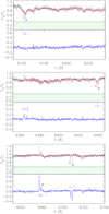 |
Fig. 4 UVES spectrum of CVSO 104 A (black dots) observed on JD = 2 459 180 in three spectral regions around 6200 Å (top), 6400 Å (middle), and 6700 Å (bottom). In each box, the synthetic spectrum, which is the weighted sum of two standard star spectra mimicking the primary and secondary component, is overplotted with a full red line. Prominent lines from the primary and secondary component are marked with a and b, respectively. The hatched green regions denote the level of the veiling. The residual spectra obtained by the subtraction of the photospheric template are displayed in the lower panel of each box with a blue line. |
 |
Fig. 5 Distribution of spectral types for the components of CVSO 104 A. |
3.4 Accretion and wind diagnostics
The residual spectra are also very helpful in measuring the equivalent widths and fluxes of emission lines of the two components when they are well separated in wavelength. We were successful in separating the contribution of the two components for He I λ5876 Å and λ6678 Å lines in all the UVES spectra, with the exception of the spectrum taken at reduced Julian date RJD = 59179, when the system was near a conjunction. We fitted two Gaussians to each spectrum to measure the centroid (RV), the FWHM, and equivalent width, Wline, of the line of each component (blue and red dashed lines in Figs. 6 and 7 for the primary and secondary component, respectively). We recover the line flux at Earth, fline, from the equivalent width Wline and the extinction corrected flux of the adjacent continuum, namely 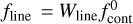 (see, e.g., Alcalá et al. 2017; Frasca et al. 2018), where the continuum flux is measured in the X-shooter spectrum10 and is corrected for the extinction by the factor 100.4Aλ, scaling Aλ from the AV = 0.35 mag (see Sect. 3.5). The line luminosity is then derived adopting the distance, d, as Lline = 4πd2fline.
The radial velocities, equivalent widths, and line luminosities are reported in Table 3, where we used the subscripts a and b for the quantities related to the primary and secondary component, respectively. A further broad emission feature, blueshifted with respect to the primary component, is visible in the He I λ5876 line at RJD = 59178. In this case, we fitted the observed line profile with three Gaussians and report the parameters of this feature (brown dashed line in Fig. 7) as RV3, W3, and  in Table 3.
The Hβ emission profiles of the two components (Fig. 8) are much wider than the He I lines and, as a consequence, they are strongly blended. However, we could still deblend them with multi-component fits of Lorentzian profiles. A third emission component is always visible out of the conjunction as a blueshifted or redshifted feature, depending on the orbital phase. It displays the maximum intensity in the first epoch (RJD = 59178), where we also observed the excess He I emission. All the three Hβ emission peaks display a much smaller intensity at RJD = 59243, although the system configuration is the same as the first epoch of UVES observations, suggesting an intrinsic accretion variation in addition to any potential geometric effect. The RV, equivalent width and line luminosity of the Hβ emission components are also quoted in Table 3.
We cannot distinguish the emission contribution of the two stars in the Hα line (Fig. A.4), but we always see the blueshifted and redshifted excess component at a velocity that is similar to that of Hβ. A two-Gaussian fit has allowed us to separate the contribution of the latter feature from the integrated emission coming from the two stars, which we also report in Table 3. We think that this broad excess emission feature can be related to the complex structure of accretion funnels.
The strong intensity variation from the first to the last spectrum is also observed in Hα and suggests a variable accretion rate. We have calculated the accretion luminosity, Lacc, with the log Lacc– log Lline linear relations proposed by Alcalá et al. (2017). The mass accretion rate, Ṁacc, was then derived from Lacc according to:
 (1)
(1)
where R⋆ and Rin are the stellar radius and inner-disk radius (assumed to be Rin = 5R⋆), respectively (see Gullbring et al. 1998; Hartmann et al. 1998). At each epoch, we have calculated the mean values of Lacc and Ṁacc (reported in Table 4), which have been obtained averaging the individual values derived from the two He I and Hβ lines. The errors include the relative errors of the line luminosities and the standard deviation of Lacc values from the three diagnostics.
The [O I] λ6300 Å line is always observed as a single and rather symmetric feature (see Fig. 9). Its radial velocity spans from +19 to +26 km s−1, therefore, itis always close to the barycentric velocity. Its equivalent width in the UVES spectra does not change very much, being about 0.80, 0.86, 1.09, and 1.20 Å, from the first to the last epoch of UVES observations. Interestingly, it is slightly stronger when the permitted lines are weaker. The [O I] λ6363 Å line displays a similar behavior. This does not necessarily mean a real intensity variation, but it could be instead the result of a decrease of the excess continuum flux due to the accretion, namely, the veiling.
The observed profile of the [O I] λ6300 Å line displays broad wings that cannot be reproduced with a single Gaussian. We therefore interpreted them as the superposition of a narrow and a broad component, which have been fitted with Gaussians. The broad component is normally associated with magneto-hydrodynamic winds from the inner (< 1 au) disk, while the narrow one is related to photoevaporated winds originating in a much more extended region (up to 100 au, e.g., Ercolano & Pascucci 2017). The parameters of the narrow (N) and broad (B) emission component are reported in Table 5. The narrow emission component has an average width of FWHM, ≃ 44 km s−1, while it is about 288 km s−1 for the broad one. Following the prescriptions applied in different studies of forbidden emission lines (Simon et al. 2016; McGinnis et al. 2018; Fang et al. 2018; Banzatti et al. 2019; Gangi et al. 2020), we can estimate the emission size of these components under the assumption that the line widths are dominated by Keplerian broadening. Assuming an inclination of i = 43 ° and a total mass of 1 M⊙ (Sect. 3.5), the narrow component should be emitted by a region of ≈0.84 au (180 R⊙), which is compatible with a circumbinary disk, as has also been found from the SED analysis. The size of the source of the broad component should be ≈ 0.02 au (4.3 R⊙).
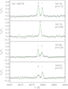 |
Fig. 6 Residual UVES spectra in the He Iλ6678 Å region (black dots). In each panel, the two-Gaussian fit to the emission peaks (green full line) and the individual Gaussians corresponding to the primary (blue dashed line) and secondary (red dashed line) component are overlaid. The blue and red vertical ticks mark the expected position of the lines of primary and secondary component, respectively, according to the photospheric RV. The reduced Julian day and the orbital phase (ϕ) are marked in the upper right corner of each box. |
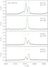 |
Fig. 7 Residual UVES He Iλ5876 Å profiles (black dots). In each panel, the two-Gaussian fit to the emission peaks (green full line) and the individual Gaussians corresponding to the primary (blue dashed line) and secondary (red dashed line) component are overlaid. The blue and red vertical ticks mark the expected position of the lines of primary and secondary component, respectively, according to the photospheric RV. The dashed brown line in the upper panel represents the Gaussian fitted to the excess blueshifted emission observed only in this spectrum. The reduced Julian day and the orbital phase (ϕ) are marked in the upper right corner of each box. |
3.5 Spectral energy distribution
To study the shape of the spectral energy distribution (SED) of CVSO 104 A, excluding the contribution of the optical companion, we used both the OACT photometry and synthetic photometry made on the flux-calibrated X-shooter spectra of the two stars (see Fig. 10). We extended the SED to mid-infrared (MIR) and far-infrared (FIR) wavelengths by adding flux values from the literature. These data are quoted in Table A.1. As the contribution of the visual companion B is strongly decreasing at longer wavelengths (see Fig. 10), we assign the MIR (WISE) and FIR (Herschel) fluxes to the component A.
To reproduce the photospheres of the two components of the binary, we combined two BT-Settl spectra (Allard et al. 2012) adopting the temperatures and flux contributions at red wavelengths, wa and wb, found with COMPO2 and reported in Table 2. With this photospheric template, we fitted the optical-NIR portion (from B to H band) of the SED (Fig. 11), fixing the Gaia EDR3 parallax and letting the extinction, AV, and the radius of the primary component, Ra, free to vary untila minimum χ2 is attained. We found AV = 0.35 mag and Ra = 1.07R⊙. The 3D extinction map of the Galaxy published by Green et al. (2019) provides E(g − r) = 0.12 mag at the position and distance of CVSO 104 A11, which translates into E(B − V) = 0.106–0.120 mag, depending on the conversion used, which would then correspond to AV = 0.33–0.37 mag. This value is in close agreement with the value of AV derived by us and suggests that most (or all) of this reddening is interstellar in nature, rather than circumstellar. The radius of the secondary component, Rb = 0.99 R⊙, is derived from Ra and the flux contributions wa and wb. We have then evaluated the stellar luminosities as L = 4πR2σTeff4. The error of luminosity includes also the error on flux contribution. These stellar parameters are also quoted in Table 2. The position of the two components of CVSO 104 A in the Hertzsprung-Russell (HR) diagram is shown in Fig. 12 along with the pre-main-sequence evolutionary tracks and isochrones by Baraffe et al. (2015). Both components lie close to the isochrone at 5 Myr and masses of 0.57 ± 0.15 M⊙ and 0.43 ± 0.15 M⊙ can be inferred for the primary and secondary component, respectively. Comparing these values with the dynamical masses reported in Table 2, we deduce a system inclination of  degrees. We note that the mass ratio derived from the position in the HR diagram, Mb ∕Ma = 0.75 ± 0.33, is smaller than but is still compatible with the dynamical one, if we take the large errors of the individual masses (± 0.15 M⊙) into account. The latter are mainly the result of the large Teff uncertainty. Therefore, the radial velocity curve strongly suggests components with closer masses and effective temperatures.
The masses and radii derived for the components Aa and Ab of CVSO 104 enable us to trace the configuration of the system, which is depicted in Fig. 13. The SED also shows that up to the H band the emission is photospheric, while longward of that it follows the typical emission pattern displayed by Class II sources in Taurus (e.g., D’Alessio et al. 1999; Furlan et al. 2006), which is outlined by the light-grey shaded area in Fig 11. Such an IR excess couldbe explained by thermal emission from a dusty disk. We can, for example, reproduce it with two blackbodies with T1 = 1000 K (red dotted line in Fig. 11) and T2 = 150 K (green dashed line). The areas of these sources, assumed as uniformly emitting, are about 1.0 × 1025 cm2 and 2.1 × 1028 cm2, respectively. If they are related to an inner and outer disk with inclination i = 43° and internal radius Rin = 1 R⊙, their radii should be ~21 and 960 R⊙. If compared with the semi-major axis  , this implies that a circumbinary disk must exist.
Multi-component analysis of permitted emission lines of CVSO 104 A in the UVES spectra.
Accretion luminosity and mass accretion rates of the components of CVSO 104 A.
Multicomponent analysis of the [O I] λ6300 Å emission line.
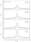 |
Fig. 9 Residual UVES spectra in the [O I] λ6300 region (black dots). The blue and red vertical ticks mark the expected position of the lines of primary and secondary component, respectively, according to the photospheric RV. The Gaussian fits to the broad and narrow component of the line profile are overplotted with purple and magenta lines, respectively, while their sum is plotted with a green line. The reduced Julian day and the orbital phase (ϕ) are marked in the upper right corner of each box. |
4 Discussion
Our study confirms that CVSO 104 A is a double-lined spectroscopic binary with a dynamical mass ratio around 0.92, which is slightly lower but marginally consistent within the uncertainties with the estimate by Kounkel et al. (2019). With an orbital period of five days, but no physical companion detected directly, by Gaia nor by Broadening Function method, the system is a rare case of a close binary without a detected tertiary component. Indeed, Laos et al. (2020) found that 90% of spectroscopic binaries with orbital periods between 3 and 6 days had a tertiary companion.
Observations with TESS reveal variability, with an irregular, or at most a semi-regular, pattern. The fact that TESS has large pixels, so that the component B is also contributing to the flux, makes difficult assessing the real amplitude of the variations and whether they really originate from the spectroscopic binary. However, according to our classification as a slowly rotating, low-activity G2 V star and the photometry displayed in Fig. A.2, the brightness variations of the component B are negligible in comparison with CVSO 104 A. The observed variations look more like small-amplitude bursts (perhaps linked to accretion) than dips, especially in the second TESS light curve, simultaneous with PENELLOPE. The TESS light curves are reminiscent of the sources in NGC 2264 with “aperiodic accretion variability” or “stochastic variability” presented by Stauffer et al. (2016) or to the “stochastic” or “burster” type of variability detected with K2 in Upper Sco (Cody & Hillenbrand 2018). With the aim of distinguishing between a “dipper” or “bursting” light curve on more quantitative grounds, we have evaluated the asymmetry of the TESS light curve, using the metric, M, expressed by Cody et al. (2014) in their Eq. (7). After removing the linear trend, we found M ≃ 0.13. According to Cody et al. (2014), values of M < −0.25 are typical of “bursting” light curves, M > +0.25 correspond to “dippers”, while −0.25 < M < +0.25 indicates symmetric light curves. As a further test, we calculated the third moment (skewness) as − 0.45, which also indicates a rather symmetric light curve. We repeated this analysis with the ASAS-SN g′ data, which have a precision and cadence lower than TESS, but a longer time baseline and we found M ≃ 0.17 and skewness −0.30, which also suggest a symmetric light curve. Therefore, we cannot classify CVSO 104 A either as a burster or a dipper. The stochastic variability is probably related to fluctuating accretion. However, our multiband photometry (Fig. A.1) shows at least two clearly detected bursts simultaneous with the enhancements of the TESS light curve. The intensification is stronger in the bluer bands, as usually observed during accretion bursts (see, e.g., Tofflemire et al. 2017).
In Paper I, we quote a mass for the star of 0.37 M⊙ and a mass accretion rate of 3.24 × 10⁻⁹ M⊙ yr−1, but these values assumed that the object was single. The mass accretion rate reported in Paper I is higher than the Ṁacc values of each component, but it is close to their sum at RJD=59178, Ṁacc ≃ 2.95 × 10⁻⁹M⊙ yr−1.
Using evolutionary tracks and isochrones of Baraffe et al. (2015), we found that both components are near the isochrone at 5 Myr and derived the masses to be 0.57 ± 0.15 M⊙ and 0.43 ± 0.15 M⊙, with a binary inclination of i ≃ 43° ± 6° (see Fig. 12). However, apart from the large mass errors, which mainly stem from the large uncertainties of Teff values, the masses depend on the adopted set of evolutionary tracks. To evaluate the impact of different models on the determination of masses and age, we have also used the SPOTS Models of Somers et al. (2020), which include the effects of magnetic activity and starspots on the structure of active stars. The HR diagrams with the Somers et al. (2020) tracks for a spot covering fraction of 0%, 34%, and 51% are shown in Fig. A.5. We note that the position of the two components with respect to the tracks with a spot filling factor Fspot = 0 is the same as for the tracks of Baraffe et al. (2015). A spot coverage of 34% would increase the masses by a factor of ~ 1.3, which is inside the mass errors, while a larger spot filling factor, Fspot = 51%, would make the masses larger by a factor ~ 1.5 and the inclination of the system would be i ≃ 37°. However, unless the spots are evenly distributed over the surface of the two stars, there is no indication of such a high coverage from the light curve which should have shown a large-amplitude rotational modulation superimposed to the observed bursts. Moreover, in the latter case, the age of the system would turn out to be 15–20 Myr, which is hardly compatible with the high mass accretion rate and with the age of ~ 5 Myr of the Ori OB1 association.
If we use the radii and orbital period listed in Table 2, we find equatorial rotation velocities of veq = 10.7 and 10.0 km s−1 for the primary and secondary components, respectively, which become v sin i =7.3 and 6.8 km s−1, that is, they are in agreement with the measured vsin i, within the errors. We therefore conclude that the components are synchronized or close to synchronization, but the system is not yet circularized. This is in agreement with the timescales for circularization and synchronization, τcirc ~ 800 Myr and τsync ~ 2 Myr, which we have calculated according to Zahn (1989). With an age of ~ 5 Myr, this system should have had time enough to synchronize the rotation of the two components with the orbital period. However, as pointed out by Hut (1981), in an eccentric orbit the tidal interaction is stronger at periastron, when the orbital velocity is higher, with the consequence that the equilibrium is reached at a value of rotation period, Ppseudo, which is smaller than Porb, leading to a pseudo-synchronization. The value of Ppseudo depends on the eccentricity of the system and results to be about 2.5 days for both components of CVSO 104 A, which is not consistent with the vsin i values measured by us. The timescale for the pseudo-synchronization can be evaluated as τpseudo ~ 12 Myr, following the guidelines of Hut (1981). This suggests that the pseudo-synchronization equilibrium has not yet been attained for the components of CVSO 104 A.
With a semi-major axis of about 13 R⊙ and an inclination of about 43°, the system should certainly not show any eclipses. In all cases, the Roche lobe radius of both stars is about 5 R⊙, that is, much larger than the radius of the individual stars, which is about 1 R⊙ (see also Fig. 13). Thus, there is also a place for circumstellar accretion disks, in addition to a circumbinary disk. The existence of the latter is confirmed by our SED analysis.
The accretion luminosities and mass accretion rates of the two components, calculated from the fluxes of the lines where the profiles of the two components could be deblended (He Iλ6678, He Iλ5876, and Hβ), are similar. The secondary component seems to accrete slightly more than the primary, but at the first epoch (RJD=59178) we see the reverse. However, these variations are within the errors and cannot be considered to be highly significant.
The numerical simulations of circumbinary accretion onto eccentric and circular binaries made by Muñoz & Lai (2016) show that for circular binaries one expects accretion bursts with a period ~ 5Porb, while for eccentric orbits it is mostly modulated at ~1Porb. This seems to be the case with CVSO 104 A, according to what is observed in the TESS light curve (Fig. 1). Moreover, based on the above simulations, the two components should have similar accretion rates in circular orbits, while very different accretion rates, with a ratio up to 10–20, should be observed in the components of binaries with eccentric orbits. The asymmetry breaking between the stars, however, alternates over timescales on the order of 200 Porb and it can be attributed to a slowly precessing, eccentric circumbinary disk. Our spectroscopic observations always display very similar Ṁacc for the two components, with some hint of variation, but they span a too small time range and further observations are needed to search for variations on 100 day timescales.
Figure 1of Muñoz & Lai (2016) clearly shows the spiral pattern of matter from the circumbinary disk to the stars and circumstellar disks. Similar structures are found in the simulations of Gillen et al. (2017) and de Val-Borro et al. (2011) for the two gas streams passing the co-linear Lagrangian points on the way down to the stars. Also, de Val-Borro et al. (2011) used their model to estimate the RV of Balmer line emission from the region within the circumbinary disk, finding maximum velocities of about ± 100 km s−1 around the quadratures, which are in agreement with the excess emission observed on V4046 Sgr by Stempels & Gahm (2004). According to Stempels & Gahm (2004), these excess emissions are consistent with two concentrations of gas co-rotating with the stars and moving with a projected velocity of 80 km s−1 around the center of mass. This suggests that they are located well inside the edge of the circumbinary disk and also inside the co-linear Lagrangian points of V4046 Sgr. It is possible that a similar accretion structure that brings matter towards the primary component is responsible for the extra emission component observed in Hα and Hβ. We note that its RV is approximately symmetric with respect to the barycentric velocity γ = 24.5 km s−1. If we are looking at the same structure at opposite phases (near quadratures) and if we assume it as quasi-stationary in the reference frame rotating with the system, it should be located at ≈ 15 R⊙ from the barycenter, that is, near the Lagrangian point L3 (see Fig. 13). The absence of a similar structure on the side of the secondary star is not an unexpected result, since the simulations of de Val-Borro et al. (2011) and Muñoz & Lai (2016) show that the density distribution in the inner gap can be highly asymmetrical. For instance, the model of Terquem et al. (2015) applied to CoRoT 223992193, a PMS binary with Porb ≃ 3.87 day and M-type components, shows that the stream of matter from the circumbinary disk to the primary is much denser than the one directed toward the secondary component. A similar result is also reported by Gómez de Castro et al. (2020) for simulations of AK Sco, a short-period SB2 composed of mid-F stars with a circumbinary disk. These authors observed an enhancement of the accretion rate during the periastron passages from UV tracers and the higher resolution COS spectra revealed that the flow was channeled preferentially into one of the two components.
Contrary to what observed by Gómez de Castro et al. (2020) for AK Sco, Ardila et al. (2015) do not detect any clear correlation between accretion luminosity and phase for the two binaries DQ Tau and UZ Tau either from UV continuum or C IV line flux, suggesting that gas is stored in the system throughout the orbit and may accrete stochastically. These systems are both composed of early-M type stars in eccentric orbits with longer orbital periods (Porb = 15.8 and 19.1 day, respectively) and circumbinary disks. However, optical emission lines and continuum veiling intensification near the periastron passage have been reported for DQ Tau (e.g., Mathieu et al. 1997; Basri et al. 1997). Kóspál et al. (2018) analyzed contemporaneous ground-based, Spitzer, and K2 photometry of DQ Tau. The K2 light curve displays a clear rotational modulation which is crossed by short-duration flare-like events but also by stronger brightening events with a complex behaviour and a longerduration, which are observed only at phases close to the periastron passage. The latter are interpreted as accretion bursts. Tofflemire et al. (2017) observed accretion bursts near periastron passages in the same binary system with multiband photometry which are stronger in the bluer bands. We observed a similar color behaviour for the bursts observed in CVSO 104 A, but they are not seen near periastron passages. Another system for which accretion burst have been observed near periastron passages is TWA 3A (Tofflemire et al. 2019). This is apparent from their U-band light curve, but it is also indicated by the intensity and FWHM of Hα, Hβ, and He I λ5876 lines, whichincrease near the periastron passages. They also show that the He I λ5876 line indicates that the primary is accreting more than the secondary and suggest that this can be explained by the Muñoz & Lai (2016) simulations. We note, however, that Porb and eccentricity are larger for TWA 3A than for CVSO 104 A, with periastron and apastron separations of 14.7 and 64.0 R⊙, respectively.Therefore the effect of periastron passage may be stronger for the former system. We need time-series high-resolution spectroscopy, possibly in different epochs, to investigate the behavior of accretion variability in CVSO 104 A.
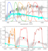 |
Fig. 10 X-shooter flux-calibrated spectrum of CVSO 104 A (pink line), CVSO 104 B (cyan line), and the sum of the two (grey line) in the visual (top panel) and NIR region (bottom panel). The contemporaneous photometry obtained from OACT in the BV RC ICz′ bands and the 2MASS JHKs photometry are displayed with colored dots. The filter bandpasses and the synthetic photometry (open squares) obtained integrating the combined spectrum (A+B) over these bandpasses are overlaid with the same color as the photometric points. |
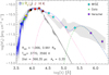 |
Fig. 11 Spectral energy distribution of CVSO 104 A based on OACT and synthetic photometry made on the X-shooter spectrum. Gaia magnitudes, mid- and far-infrared fluxes are shown with different symbols, as indicated in the legend. The combination of BT-Settl spectra (Allard et al. 2012) that reproduce the photospheres of the components of the close binary is shown by a gray line. The two black bodies with T = 1000 K and T = 150 K that fit the MIR and FIR disk emission are shown by the dotted red and dashed green lines, respectively. The continuous blue line displays the sum of the smoothed photospheric template and the two black bodies. The light-grey shaded area in the background is the median SED of Class II Taurus sources according to D’Alessio et al. (1999) and Furlan et al. (2006), reddened by AV = 0.35 mag, and scaled to the H band photometric point. |
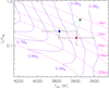 |
Fig. 12 Position of the primary (blue dot) and secondary (red dot) component of CVSO 104 A in the HR diagram. Isochrones and evolutionary tracks by Baraffe et al. (2015) are overlaid as dashed and solid lines; the labels represent their age and mass. The green asterisk connected with green dotted lines to the dots marks the position of CVSO 104 A, with the parameters derived from the combined spectrum in Paper I. |
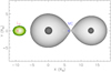 |
Fig. 13 Schematic representation of the geometry of the CVSO 104 A system in the orbital plane. The dark shaded surfaces represent the primary (at left) and secondary component, while the light-grey one is the critical Roche surface. The size and separation of the stars and Roche lobes as well as the position of the barycenter (MC) and the Lagrangian point L3 are to scale. The source of the excess Hα and Hβ emission is represented by the shaded green area. |
5 Conclusions
We presented a spectroscopic and photometric study of the PMS object CVSO 104 A, which is located in the Ori OB1 association and has an optical companion with a similar brightness at about 2 . The latter star, which we have named CVSO 104 B, is a background Sun-like star not physically associated with the PMS object and does not belong to Ori OB1. Thanks to high- and intermediate-resolution spectra taken in the framework of the PENELLOPE large program and archival APOGEE spectra, we confirmed CVSO 104 A as a double-lined spectroscopic binary and derived, for the first time, its orbital parameters. We found a dynamical mass ratio of 0.92, an orbital period of about five days, and an eccentric orbit (e ≃ 0.39, see Table 2). It is a rare case of a close binary without a detected tertiary component.
The analysis of the UVES spectra also allowed us to estimate the parameters of the two components of the binary system, which turn out to be slowly rotating (v sin i ≃ 6–7 km s−1), early M-type stars. In the HR diagram, both stars are located near the same isochrone at 5 Myr (according to two different models), which is in good agreement with the age estimated for Ori OB1. The rotation rates indicate that the two stars have already attained spin-orbit synchronization but the orbit is not yet circular. This agrees with the timescales for synchronization and circularization that we have estimated as τsync ~ 2 Myr and τcirc ~ 800 Myr, respectively.
The SED shows a significant infrared excess that can be explained only with a circumbinary accretion disk with an extension of at least 4.5 au (960 R⊙), although the presence of circumstellar disks around the two stars cannot be ruled out. The kinematic properties (RV and FWHM) of the narrow component of the [O I] λ6300Å line are also compatible with emission from a region of a circumbinary disk of ≈1 au.
The analysis of permitted lines, such as Hβ, He I λ5876 Å, and He I λ6678 Å, after the removal of the underlying photospheric spectrum, clearly reveals emission from both components of the close binary CVSO 104 A with a similar intensity. This result is in contrast with what is suggested by some theoretical studies, which predict, for most of the time, very different accretion rates for the components of an eccentric binary system, even if they have a similar mass (e.g., Muñoz & Lai 2016). However, since the ratio of accretion rates of the components is expected to reverse periodically, a binary system should be observed nearly-continuously for a long time (≳ 100 days) to draw firm conclusions. In addition to the emission profiles corresponding to the velocity of the components and likely produced by emitting material near the accretion shocks, the Hα and Hβ profiles display a broad excess emission component, which appears blueshifted or redshifted by more than 100 km s−1 at different phases. We think that this emission could be produced by an accretion funnel from the circumbinary disk towards the primary component, similar to what was found by Stempels & Gahm (2004) for V4046 Sgr and in agreement with the predictions from the numerical simulations (e.g., de Val-Borro et al. 2011; Terquem et al. 2015; Gillen et al. 2017).
The contemporaneous space- (TESS) and ground-based photometry displays a stochastic variability pattern with a possible periodicity around 4.7 days (not far from the orbital period) and some short-duration (≈1 day) peaks. The latter are reminiscent of accretion bursts, based on their shape and color dependence. However, unlike other binary systems with eccentric orbits (such as the paradigmatic case of DQ Tau), these accretion bursts do not seem to occur near the periastron passages.
Future studies with multi-epochs and high-resolution spectroscopy of this and other PMS binaries are needed for a deeper investigation of the impact of multiplicity on the mass accretion phenomenon. The synergy between ODYSSEUSand PENELLOPE large programs can be of great assistance in this respect, with the data being publicly available12.
Acknowledgements
We thank the anonymous referee for her/his useful comments and suggestions. We acknowledge the support from the Italian Ministero dell’Istruzione, Università e Ricerca (MIUR). This work has been partially supported by the project PRIN-INAF-MAIN-STREAM 2017 “Protoplanetary disks seen through the eyes of new-generation instruments” and from the project PRIN-INAF 2019 “Spectroscopically Tracing the Disk Dispersal Evolution”. This work benefited from discussions with the ODYSSEUS team (HST AR-16129), https://sites.bu.edu/odysseus/. This project has received funding from the European Union’s Horizon 2020 research and innovation programme under the Marie Skłodowska-Curie grant agreement No. 823823 (DUSTBUSTERS). This project has received funding from the European Research Council (ERC) under the European Union’s Horizon 2020 research and innovation programme under grant agreement No 716155 (SACCRED). This work was partly supported by the Deutsche Forschungs-Gemeinschaft (DFG, German Research Foundation) – Ref no. FOR 2634/1 TE 1024/1-1. F.M.W. is grateful to the AAVSO for the award of AAVSOnet telescope time, and to the Ken Menzies for implementing the observations. We thank Elizabeth Waagen and the citizen scientists of the AAVSO for their contributions to this program. K.G. acknowledges the partial support from the Ministry of Science and Higher Education of the Russian Federation (grant 075-15-2020-780). This research made use of SIMBAD and VIZIER databases, operated at the CDS, Strasbourg, France, and of LIGHTKURVE, a Python package for Kepler and TESS data analysis (Lightkurve Collaboration 2018).
Appendix A Additional tables and figures
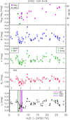 |
Fig. A.1 Multiband ground-based light curve of CVSO 104 A+B around the time of VLT and HST observations. Different symbols, as reported in the legend, are used for the different data sets. The Hα color index, which measures the intensity of the line, is shown in the upper panel. Synthetic Hα colors based on X-shooter and UVES spectra are overplotted with asterisks in the same box. The contemporaneous TESS light curve is overplotted with grey dots to the RC light curve. The arrows in the same box mark the periastron passages. The epoch of VLT and HST observations are marked in the lower box. |
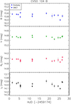 |
Fig. A.2 Multiband ground-based photometry of CVSO 104 B obtained at OACT and Konkoly observatories in the nights with a good seeing. |
Photometry of CVSO 104 A and B.
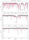 |
Fig. A.3 UVES spectrum of CVSO 104 B (black dots) in three spectral regions around the Mg I b triplet (top), Hα (middle), and 6700 Å (bottom). In each box the spectrum of the standard star that is best fitting that of CVSO 104 B is overplotted with a full red line. |
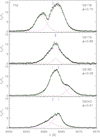 |
Fig. A.4 Residual UVES Hα profiles (black dots). The totally blended emission from the two stars is represented, in each box, by a magenta dashed line, while the brown dashed line is the Gaussian fitted to the excess blueshifted or redshifted emission. The sum of the two Gaussians is overplotted as a full green line. The blue and red vertical ticks mark the expected position of the lines of primary and secondary component, respectively, according to the photospheric RV. |
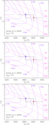 |
Fig. A.5 HR diagram of the primary (blue dot) and secondary (red dot) component of CVSO 104 A with isochrones and evolutionarytracks by Somers et al. (2020) for three spot covering factors. |
References
- Ahumada, R., Prieto, C. A., Almeida, A., et al. 2020, ApJS, 249, 3 [Google Scholar]
- Alcalá, J. M., Manara, C. F., Natta, A., et al. 2017, A&A, 600, A20 [NASA ADS] [CrossRef] [EDP Sciences] [Google Scholar]
- Allard, F., Homeier, D., & Freytag, B. 2012, Phil. Trans. Roy. Soc. Lond. A, 370, 2765 [Google Scholar]
- Ardila, D. R., Jonhs-Krull, C., Herczeg, G. J., Mathieu, R. D., & Quijano-Vodniza, A. 2015, ApJ, 811, 131 [NASA ADS] [CrossRef] [Google Scholar]
- Banzatti, A., Pascucci, I., Edwards, S., et al. 2019, ApJ, 870, 76 [Google Scholar]
- Baraffe, I., Homeier, D., Allard, F., & Chabrier, G. 2015, A&A, 577, A42 [NASA ADS] [CrossRef] [EDP Sciences] [Google Scholar]
- Basri, G., Johns-Krull, C. M., & Mathieu, R. D. 1997, AJ, 114, 781 [NASA ADS] [CrossRef] [Google Scholar]
- Bevington, P. R., & Robinson, D. K. 2003, Data reduction and error analysis for the physical sciences (Boston, MA: McGraw-Hil) [Google Scholar]
- Briceño, C., Calvet, N., Hernández, J., et al. 2005, AJ, 129, 907 [Google Scholar]
- Cody, A. M., & Hillenbrand, L. A. 2018, AJ, 156, 71 [Google Scholar]
- Cody, A. M., Stauffer, J., Baglin, A., et al. 2014, AJ, 147, 82 [Google Scholar]
- Covino, E., Frasca, A., Alcalá, J. M., Paladino, R., & Sterzik, M. F. 2004, A&A, 427, 637 [NASA ADS] [CrossRef] [EDP Sciences] [Google Scholar]
- Cutri, R. M., Wright, E. L., Conrow, T., et al. 2021, VizieR Online Data Catalog: II/328 [Google Scholar]
- D’Alessio, P., Calvet, N., Hartmann, L., Lizano, S., & Cantó, J. 1999, ApJ, 527, 893 [CrossRef] [Google Scholar]
- de Val-Borro, M., Gahm, G. F., Stempels, H. C., & Pepliński, A. 2011, MNRAS, 413, 2679 [NASA ADS] [CrossRef] [Google Scholar]
- Dekker, H., D’Odorico, S., Kaufer, A., Delabre, B., & Kotzlowski, H. 2000, in Optical and IR Telescope Instrumentation and Detectors, eds. M. Iye, & A. F. Moorwood, SPIE Conf. Ser., 4008, 534 [NASA ADS] [Google Scholar]
- Eggleton, P. P., & Kiseleva-Eggleton, L. 2001, ApJ, 562, 1012 [NASA ADS] [CrossRef] [Google Scholar]
- Ercolano, B., & Pascucci, I. 2017, Roy. Soc. Open Sci., 4, 170114 [Google Scholar]
- Fang, M., Pascucci, I., Edwards, S., et al. 2018, ApJ, 868, 28 [NASA ADS] [CrossRef] [Google Scholar]
- Frasca, A., Guillout, P., Marilli, E., et al. 2006, A&A, 454, 301 [NASA ADS] [CrossRef] [EDP Sciences] [Google Scholar]
- Frasca, A., Biazzo, K., Lanzafame, A. C., et al. 2015, A&A, 575, A4 [NASA ADS] [CrossRef] [EDP Sciences] [Google Scholar]
- Frasca, A., Biazzo, K., Alcalá, J. M., et al. 2017, A&A, 602, A33 [NASA ADS] [CrossRef] [EDP Sciences] [Google Scholar]
- Frasca, A., Montes, D., Alcalà, J. M., Klutsch, A., & Guillout, P. 2018, Acta Astron., 68, 403 [NASA ADS] [Google Scholar]
- Furlan, E., Hartmann, L., Calvet, N., et al. 2006, ApJS, 165, 568 [NASA ADS] [CrossRef] [Google Scholar]
- Gaia Collaboration 2020, VizieR Online Data Catalog: I/350 [Google Scholar]
- Gangi, M., Nisini, B., Antoniucci, S., et al. 2020, A&A, 643, A32 [NASA ADS] [CrossRef] [EDP Sciences] [Google Scholar]
- Gillen, E., Aigrain, S., Terquem, C., et al. 2017, A&A, 599, A27 [NASA ADS] [CrossRef] [EDP Sciences] [Google Scholar]
- Gómez de Castro, A. I., Vallejo, J. C., Canet, A., Loyd, P., & France, K. 2020, ApJ, 904, 120 [CrossRef] [Google Scholar]
- Green, G. M., Schlafly, E., Zucker, C., Speagle, J. S., & Finkbeiner, D. 2019, ApJ, 887, 93 [NASA ADS] [CrossRef] [Google Scholar]
- Gullbring, E., Hartmann, L., Briceño, C., & Calvet, N. 1998, ApJ, 492, 323 [Google Scholar]
- Haro, G., & Moreno, A. 1953, Boletin Observ. Tonantz. Tacubaya, 1, 11 [Google Scholar]
- Hartmann, L., Calvet, N., Gullbring, E., & D’Alessio, P. 1998, ApJ, 495, 385 [Google Scholar]
- Henden, A. A., Levine, S., Terrell, D., et al. 2018, in Amer. Astron. Soc. Meet. Abstr., 232, 223.06 [Google Scholar]
- Herschel Point Source Catalogue Working Group, Marton, G., Calzoletti, L., et al. 2020, VizieR Online Data Catalog: VIII/106 [Google Scholar]
- Hillenbrand, L. A., & White, R. J. 2004, ApJ, 604, 741 [NASA ADS] [CrossRef] [Google Scholar]
- Hut, P. 1981, A&A, 99, 126 [NASA ADS] [Google Scholar]
- Jönsson, H., Holtzman, J. A., Allende Prieto, C., et al. 2020, AJ, 160, 120 [Google Scholar]
- Karim, M. T., Stassun, K. G., Briceño, C., et al. 2016, AJ, 152, 198 [NASA ADS] [CrossRef] [Google Scholar]
- Kóspál, Á., Ábrahám, P., Zsidi, G., et al. 2018, ApJ, 862, 44 [CrossRef] [Google Scholar]
- Kounkel, M., Covey, K., Moe, M., et al. 2019, AJ, 157, 196 [NASA ADS] [CrossRef] [Google Scholar]
- Laos, S., Stassun, K. G., & Mathieu, R. D. 2020, ApJ, 902, 107 [NASA ADS] [CrossRef] [Google Scholar]
- Lightkurve Collaboration, (Cardoso, J. V. d. M.,) et al. 2018, Lightkurve: Kepler and TESS time series analysis in Python, Astrophysics Source Code Library [Google Scholar]
- Manara, C. F., Frasca, A., Venuti, L., et al. 2021, A&A, 650, A196, (Paper I) [NASA ADS] [CrossRef] [EDP Sciences] [Google Scholar]
- Mathieu, R. D., Stassun, K., Basri, G., et al. 1997, AJ, 113, 1841 [NASA ADS] [CrossRef] [Google Scholar]
- McGinnis, P., Dougados, C., Alencar, S. H. P., Bouvier, J., & Cabrit, S. 2018, A&A, 620, A87 [NASA ADS] [CrossRef] [EDP Sciences] [Google Scholar]
- Muñoz, D. J., & Lai, D. 2016, ApJ, 827, 43 [Google Scholar]
- Naoz, S., & Fabrycky, D. C. 2014, ApJ, 793, 137 [Google Scholar]
- Press, W. H., Teukolsky, S. A., Vetterling, W. T., & Flannery, B. P. 1992, Numerical recipes in FORTRAN. The art of scientific computing (Cambridge: University Press) [Google Scholar]
- Ricker, G. R., Winn, J. N., Vanderspek, R., et al. 2015, J. Astron. Telescopes Instrum. Syst., 1, 014003 [Google Scholar]
- Roberts, D. H., Lehar, J., & Dreher, J. W. 1987, AJ, 93, 968 [Google Scholar]
- Roman-Duval,J., Proffitt, C. R., Taylor, J. M., et al. 2020, Res. Notes Am. Astron. Soc., 4, 205 [Google Scholar]
- Rucinski, S. M. 2012, in From Interacting Binaries to Exoplanets: Essential Modeling Tools, eds. M. T. Richards & I. Hubeny, 282, 365 [NASA ADS] [Google Scholar]
- Scargle, J. D. 1982, ApJ, 263, 835 [Google Scholar]
- Simon, M. N., Pascucci, I., Edwards, S., et al. 2016, ApJ, 831, 169 [Google Scholar]
- Somers, G., Cao, L., & Pinsonneault, M. H. 2020, ApJ, 891, 29 [Google Scholar]
- Stassun, K. G., Feiden, G. A., & Torres, G. 2014, New A Rev., 60, 1 [CrossRef] [Google Scholar]
- Stauffer, J., Cody, A. M., Rebull, L., et al. 2016, AJ, 151, 60 [NASA ADS] [CrossRef] [Google Scholar]
- Stempels, H. C., & Gahm, G. F. 2004, A&A, 421, 1159 [NASA ADS] [CrossRef] [EDP Sciences] [Google Scholar]
- Terquem, C., Sørensen-Clark, P. M., & Bouvier, J. 2015, MNRAS, 454, 3472 [NASA ADS] [CrossRef] [Google Scholar]
- Tofflemire, B. M., Mathieu, R. D., Ardila, D. R., et al. 2017, ApJ, 835, 8 [CrossRef] [Google Scholar]
- Tofflemire, B. M., Mathieu, R. D., & Johns-Krull, C. M. 2019, AJ, 158, 245 [NASA ADS] [CrossRef] [Google Scholar]
- Tokovinin, A., Petr-Gotzens, M. G., & Briceño, C. 2020, AJ, 160, 268 [NASA ADS] [CrossRef] [Google Scholar]
- Tonry, J., & Davis, M. 1979, AJ, 84, 1511 [Google Scholar]
- Vernet, J., Dekker, H., D’Odorico, S., et al. 2011, A&A, 536, A105 [NASA ADS] [CrossRef] [EDP Sciences] [Google Scholar]
- Wiramihardja,S. D., Kogure, T., Yoshida, S., Ogura, K., & Nakano, M. 1989, PASJ, 41, 155 [NASA ADS] [Google Scholar]
- Zahn, J. P. 1989, A&A, 220, 112 [Google Scholar]
- Zapatero Osorio, M. R., Béjar, V. J. S., Pavlenko, Y., et al. 2002, A&A, 384, 937 [NASA ADS] [CrossRef] [EDP Sciences] [Google Scholar]
- Zrake, J., Tiede, C., MacFadyen, A., & Haiman, Z. 2021, ApJ, 909, L13 [NASA ADS] [CrossRef] [Google Scholar]
Available at http://skyserver.sdss.org/dr16/
Available at https://www.aavso.org/data-download
IRAF is distributed by the National Optical Astronomy Observatory, which is operated by the Association of Universities for Research in Astronomy, Inc.
IDL (Interactive Data Language) is a registered trademark of Harris Corporation.
A small correction was applied to the continuum flux based on the photometric variations.
All Tables
Multi-component analysis of permitted emission lines of CVSO 104 A in the UVES spectra.
All Figures
|
Fig. 1 TESS light curves of CVSO 104 A+B in 2018 (top) and 2020 (bottom). |
| In the text | |
|
Fig. 2 Portion of images acquired at OACT on 16 December 2020 in BV RI bands centered on the visual pair CVSO 104 A+B. North is up and east is to the left and the two components are indicated in the R-band image. We note how the relative brightness of the two stars changes in the different bands, with A becoming brighter than B in the I band. |
| In the text | |
|
Fig. 3 Heliocentric radial velocity curve (circles = UVES, squares = APOGEE, diamonds = X-shooter data) of CVSO 104 A. Filled and open symbols have been used for the primary (more massive) and secondary component, respectively.The blue and red lines represent the orbital solution (Table 2) for the primary and secondary component, respectively. |
| In the text | |
|
Fig. 4 UVES spectrum of CVSO 104 A (black dots) observed on JD = 2 459 180 in three spectral regions around 6200 Å (top), 6400 Å (middle), and 6700 Å (bottom). In each box, the synthetic spectrum, which is the weighted sum of two standard star spectra mimicking the primary and secondary component, is overplotted with a full red line. Prominent lines from the primary and secondary component are marked with a and b, respectively. The hatched green regions denote the level of the veiling. The residual spectra obtained by the subtraction of the photospheric template are displayed in the lower panel of each box with a blue line. |
| In the text | |
|
Fig. 5 Distribution of spectral types for the components of CVSO 104 A. |
| In the text | |
|
Fig. 6 Residual UVES spectra in the He Iλ6678 Å region (black dots). In each panel, the two-Gaussian fit to the emission peaks (green full line) and the individual Gaussians corresponding to the primary (blue dashed line) and secondary (red dashed line) component are overlaid. The blue and red vertical ticks mark the expected position of the lines of primary and secondary component, respectively, according to the photospheric RV. The reduced Julian day and the orbital phase (ϕ) are marked in the upper right corner of each box. |
| In the text | |
|
Fig. 7 Residual UVES He Iλ5876 Å profiles (black dots). In each panel, the two-Gaussian fit to the emission peaks (green full line) and the individual Gaussians corresponding to the primary (blue dashed line) and secondary (red dashed line) component are overlaid. The blue and red vertical ticks mark the expected position of the lines of primary and secondary component, respectively, according to the photospheric RV. The dashed brown line in the upper panel represents the Gaussian fitted to the excess blueshifted emission observed only in this spectrum. The reduced Julian day and the orbital phase (ϕ) are marked in the upper right corner of each box. |
| In the text | |
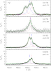 |
Fig. 8 Residual UVES Hβ profiles (black dots). The meaning of the symbols is as in Fig. 7. |
| In the text | |
|
Fig. 9 Residual UVES spectra in the [O I] λ6300 region (black dots). The blue and red vertical ticks mark the expected position of the lines of primary and secondary component, respectively, according to the photospheric RV. The Gaussian fits to the broad and narrow component of the line profile are overplotted with purple and magenta lines, respectively, while their sum is plotted with a green line. The reduced Julian day and the orbital phase (ϕ) are marked in the upper right corner of each box. |
| In the text | |
|
Fig. 10 X-shooter flux-calibrated spectrum of CVSO 104 A (pink line), CVSO 104 B (cyan line), and the sum of the two (grey line) in the visual (top panel) and NIR region (bottom panel). The contemporaneous photometry obtained from OACT in the BV RC ICz′ bands and the 2MASS JHKs photometry are displayed with colored dots. The filter bandpasses and the synthetic photometry (open squares) obtained integrating the combined spectrum (A+B) over these bandpasses are overlaid with the same color as the photometric points. |
| In the text | |
|
Fig. 11 Spectral energy distribution of CVSO 104 A based on OACT and synthetic photometry made on the X-shooter spectrum. Gaia magnitudes, mid- and far-infrared fluxes are shown with different symbols, as indicated in the legend. The combination of BT-Settl spectra (Allard et al. 2012) that reproduce the photospheres of the components of the close binary is shown by a gray line. The two black bodies with T = 1000 K and T = 150 K that fit the MIR and FIR disk emission are shown by the dotted red and dashed green lines, respectively. The continuous blue line displays the sum of the smoothed photospheric template and the two black bodies. The light-grey shaded area in the background is the median SED of Class II Taurus sources according to D’Alessio et al. (1999) and Furlan et al. (2006), reddened by AV = 0.35 mag, and scaled to the H band photometric point. |
| In the text | |
|
Fig. 12 Position of the primary (blue dot) and secondary (red dot) component of CVSO 104 A in the HR diagram. Isochrones and evolutionary tracks by Baraffe et al. (2015) are overlaid as dashed and solid lines; the labels represent their age and mass. The green asterisk connected with green dotted lines to the dots marks the position of CVSO 104 A, with the parameters derived from the combined spectrum in Paper I. |
| In the text | |
|
Fig. 13 Schematic representation of the geometry of the CVSO 104 A system in the orbital plane. The dark shaded surfaces represent the primary (at left) and secondary component, while the light-grey one is the critical Roche surface. The size and separation of the stars and Roche lobes as well as the position of the barycenter (MC) and the Lagrangian point L3 are to scale. The source of the excess Hα and Hβ emission is represented by the shaded green area. |
| In the text | |
|
Fig. A.1 Multiband ground-based light curve of CVSO 104 A+B around the time of VLT and HST observations. Different symbols, as reported in the legend, are used for the different data sets. The Hα color index, which measures the intensity of the line, is shown in the upper panel. Synthetic Hα colors based on X-shooter and UVES spectra are overplotted with asterisks in the same box. The contemporaneous TESS light curve is overplotted with grey dots to the RC light curve. The arrows in the same box mark the periastron passages. The epoch of VLT and HST observations are marked in the lower box. |
| In the text | |
|
Fig. A.2 Multiband ground-based photometry of CVSO 104 B obtained at OACT and Konkoly observatories in the nights with a good seeing. |
| In the text | |
|
Fig. A.3 UVES spectrum of CVSO 104 B (black dots) in three spectral regions around the Mg I b triplet (top), Hα (middle), and 6700 Å (bottom). In each box the spectrum of the standard star that is best fitting that of CVSO 104 B is overplotted with a full red line. |
| In the text | |
|
Fig. A.4 Residual UVES Hα profiles (black dots). The totally blended emission from the two stars is represented, in each box, by a magenta dashed line, while the brown dashed line is the Gaussian fitted to the excess blueshifted or redshifted emission. The sum of the two Gaussians is overplotted as a full green line. The blue and red vertical ticks mark the expected position of the lines of primary and secondary component, respectively, according to the photospheric RV. |
| In the text | |
|
Fig. A.5 HR diagram of the primary (blue dot) and secondary (red dot) component of CVSO 104 A with isochrones and evolutionarytracks by Somers et al. (2020) for three spot covering factors. |
| In the text | |
Current usage metrics show cumulative count of Article Views (full-text article views including HTML views, PDF and ePub downloads, according to the available data) and Abstracts Views on Vision4Press platform.
Data correspond to usage on the plateform after 2015. The current usage metrics is available 48-96 hours after online publication and is updated daily on week days.
Initial download of the metrics may take a while.