© ESO 2021

1. Introduction

The statistics of fluctuations in the matter density as a function of angular scale and redshift encode information about the cosmological model. A challenge for observational studies is that most of the matter is invisible. The distribution of matter can nonetheless be revealed because the differential deflection of light rays by intervening structures introduces apparent correlations in the ellipticities of distant galaxies (see Kilbinger 2015 for a recent review), a phenomenon referred to as weak gravitational lensing. These correlations can be compared to model predictions, making weak lensing by large-scale structure, or cosmic shear, a particularly powerful tool for cosmology. Moreover, the constraining power can be enhanced when the shape measurements are combined with redshift estimates for these galaxies (e.g., Troxel et al. 2018; Asgari et al. 2021), which also enables cross-correlations between the positions of galaxies and the lensing signal (e.g., Abbott et al. 2018; Heymans et al. 2021).

Given the prospects of cosmic shear, deep imaging surveys, such as the ones by Euclid¹ (Laureijs et al. 2011) and the Nancy Grace Roman Space Telescope² (Spergel et al. 2015) from space, and the Legacy Survey of Space and Time by the Rubin Observatory³ (LSST Science Collaboration 2009) from the ground, plan to cover large fractions of the extragalactic sky, increasing the galaxy samples by more than an order of magnitude. Obtaining reliable redshift information for these sources will be challenging, but so is ensuring accurate measurements of their shapes. Here, we limit ourselves to the latter, but we note that the blending of galaxies actually makes this a joint problem (MacCrann et al. 2022).

In the case of cosmic shear, the galaxy images are slightly distorted, and the lensing signal can only be detected by averaging shape measurements of large ensembles of galaxies. The challenge is to ensure that instrumental sources of bias can be corrected for to a level that renders them subdominant to the statistical uncertainties (see Mandelbaum 2018 for a detailed review on weak lensing systematics). In particular, the measurements need to be corrected for the smearing by the point spread function (PSF) and the bias caused by noise in the images. A further complication is the interpretation of measurements of blended galaxies (e.g., Hoekstra et al. 2021; MacCrann et al. 2022). Finally, biases are generally already introduced during the object detection stage (e.g., Fenech Conti et al. 2017; Kannawadi et al. 2019; Hernández-Martín et al. 2020; Hoekstra et al. 2021).

The impact of the various sources of bias can be studied by applying the shape measurement algorithm to simulated data, where the galaxy images are sheared by a known amount. The shear biases are then determined by comparing the average inferred shear, ${\gamma }_i^{\text{obs}}$, to the input shear, ${\gamma }_i^{\text{true}}$, where the index i ∈ {1, 2} corresponds to the real or imaginary part of the shear, respectively. To first order, we can assume

$$\begin{array}{c}\hfill {\gamma }_i^{\mathrm{obs}}=(1+{\mu }_i){\gamma }_i^{\mathrm{true}}+c_i,\end{array}$$(1)

where μ_i is the multiplicative shear bias and c_i is the additive shear bias. Although μ₁ and μ₂ can differ in principle, we found them to be the same in our analysis. We therefore use the average value, μ, in the remainder of this paper.

The mean shear across a large survey is expected to vanish and thus does not contain interesting cosmological information. Instead, the cosmological information is contained in the correlations between two (or more) galaxies. Analogously, a global non-vanishing additive bias only affects the ℓ = 0 mode but does not change the corresponding cosmic shear power spectrum. In contrast, a non-vanishing mean multiplicative bias changes the amplitude of the shear power spectrum, thus biasing cosmological parameter estimation. Differences between additive and multiplicative bias also occur when we consider their spatial variations. This was demonstrated in Kitching et al. (2019) by expressing the shear field in terms of spherical harmonics. They showed that, to first order, only the average value of μ matters. In contrast, spatial variations in additive bias directly contribute to the shear power spectrum and thus should be fully corrected for. Conveniently, coherent residual additive biases can be inferred from the data as the average shear should vanish. Averaging shear estimates in a suitable frame, defined by the source of bias, then reveals how the bias varies as a function of galaxy properties and instrumental effect. Arguably, this reduces the required accuracy with which a shape measurement algorithm needs to correct for additive bias: Any residual could be ‘learned’ from the data, opening up the possibility of a data-driven correction.

This leaves the problem of the multiplicative bias because it cannot be inferred from a catalogue of shear estimates. Instead, simulated data are commonly used to infer the residual multiplicative bias as a function of galaxy properties (e.g., Hoekstra et al. 2015; Fenech Conti et al. 2017; Kannawadi et al. 2019). The fidelity of the result, however, depends crucially on the realism of the simulated data (e.g., Hoekstra et al. 2015, 2017; Euclid Collaboration 2019). This is a particular concern for upcoming surveys, for which the required accuracy is challenging.

An alternative approach, referred to as METACALIBRATION, was introduced by Huff & Mandelbaum (2017) and Sheldon & Huff (2017). These papers showed how the response to a shear for an ensemble of galaxies can be determined from the data themselves, by applying a small shear to the images whilst accounting for the smearing by the PSF. The METACALIBRATION shear estimates still suffer from detection biases (Hoekstra et al. 2021, H21 hereafter). To account for this, Sheldon et al. (2020) proposed a modification of the METACALIBRATION algorithm: METADETECTION uses the same sheared images, but both the detection and the shape analysis are performed on these images.

The prospects of this data-driven approach were explored further in H21 for a Euclid-like setup. They showed that METADETECTION yields unbiased shear estimates if the PSF is axisymmetric. In practice, the PSF will be anisotropic, leading to additive bias. As explored in Sheldon & Huff (2017), METACALIBRATION can also be used to correct for PSF anisotropy, but the estimate for individual galaxies may be too noisy to be used in practice. Moreover, the extra image manipulations add to the, already substantial, computational cost. Alternatively, the images can be convolved with a kernel that circularises the PSF, but this leads to additional smoothing and anisotropic noise that need to be accounted for. This reduces the effective data quality.

Instead, here we explore if additional image manipulations can be avoided by correcting the shape estimates for PSF anisotropy as part of the METADETECTION step. This step may not be able to remove the effects of PSF anisotropy to the required level of accuracy, but as we show, this need not be a concern, because we find that the multiplicative bias after METADETECTION is not sensitive to the PSF anisotropy itself. We exploit this to show how unbiased shear estimates can be inferred from the data alone.

We describe the shape measurement algorithm in Sect. 2. The setup to create the simulated data is described in detail in Hoekstra et al. (2017) and H21, but we review the key points in Sect. 3. In Sect. 4 we present results for Euclid-like data, and in Sect. 5 we explore the performance for ground-based data. We conclude in Sect. 6.

2. Shear estimation

One of the simplest ways to quantify the shape of a galaxy is to measure the quadrupole moments of the surface brightness distribution, and combine these into the complex polarisation (or distortion), χ = χ₁ + iχ₂, where

$$\begin{array}{c}\hfill {\chi }_1=\frac{Q_{11}-Q_{22}}{Q_{11}+Q_{22}},\mathrm{and}{\chi }_2=\frac{2Q_{12}}{Q_{11}+Q_{22}}·\end{array}$$(2)

Here, Q_ij are the (weighted) quadrupole moments, defined as

$$\begin{array}{c}\hfill Q_{\mathit{ij}}={\displaystyle \int }{\mathrm{d}}^2\mathbf{x}{x}_i{x}_{j}W(\mathbf{x})I(\mathbf{x}),\end{array}$$(3)

where I(x) is the observed surface brightness distribution of a galaxy, and we introduced a weight function W(x) to suppress the diverging contribution from noise in the observed image. This weight function is typically chosen to maximise the signal-to-noise ratio, but this is not essential: The measurement uncertainties are typically negligible compared to the intrinsic ellipticities, which dominate the uncertainty in the estimate of the weak lensing signal. In fact, a non-optimal weight function can reduce the sensitivity to poor sampling of the images (Kannawadi et al. 2021) or colour gradients (Semboloni et al. 2013), and can reduce selection biases (H21). We therefore followed H21 and adopted an isotropic Gaussian with a fixed value for the dispersion of σ_w, irrespective of the size of the galaxy.

If a shear, γ = γ₁ + iγ₂ is applied to an image⁴, the observed polarisation changes, and in the case of unweighted moments, the observed value is given by (Seitz & Schneider 1997)

$$\begin{array}{c}\hfill \chi =\frac{{\chi }^{\text{int}}+2\gamma +{\gamma }^2{{\chi }^{\text{int}}}^{\ast }}{1+{\gamma }^{\ast }\gamma +({\gamma }^{\ast }{\chi }^{\text{int}}+\gamma {{\chi }^{\text{int}}}^{\ast })},\end{array}$$(4)

where χ^int denotes the intrinsic polarisation of a galaxy, and ^* indicates the complex conjugate. In practice, the challenge is to relate the observed (weighted) polarisations to the true values for ensembles of galaxies, because we need to correct for both the weight function and the smearing by the PSF. This is trivial for unweighted moments because 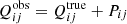$Q_{\mathit{ij}}^{\mathrm{obs}}=Q_{\mathit{ij}}^{\mathrm{true}}+P_{\mathit{ij}}$, where P_ij are the unweighted quadrupole moments of the PSF. In the case of weighted quadrupole moments, however, the correction requires the computation of higher-order moments of the surface brightness distribution.

It is convenient to consider the PSF correction as a two-step process: The first step removes the anisotropy introduced by the PSF, and the second step corrects the result for the isotropic blurring by the PSF. This is the approach used by the well-known KSB algorithm (Kaiser et al. 1995; Luppino & Kaiser 1997; Hoekstra et al. 1998). If we know the response of a galaxy image to these steps, we can undo the bias that is introduced. This is precisely what METACALIBRATION and METADETECTION provide. Given the unprecedented performance for isotropic PSFs, we used METADETECTION here to determine the multiplicative bias, but we explored an alternative approach to account for the PSF anisotropy.

The change in the observed polarisation of a galaxy due to PSF anisotropy, δχ_i, can be expressed as:

$$\begin{array}{c}\hfill \delta {\chi }_i^{=}{\chi }_i^{\mathrm{obs}}-{\chi }_i^{\mathrm{iso}}\equiv P_{\mathit{ii}}^{\mathrm{sm}}{\chi }_i^{\mathrm{PSF}},\end{array}$$(5)

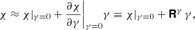
where ${\chi }_i^{\text{iso}}$ is the polarisation in the absence of PSF anisotropy, ${\chi }_i^{\text{PSF}}$ is the polarisation of the PSF, and $P_{\mathit{ii}}^{\mathrm{sm}}$ is the smear polarisability. Formally, it is a 2 × 2 tensor, but as off-diagonal terms are small in general, and vanish for ensemble averages, we only considered the diagonal elements.

Kaiser et al. (1995) derived an approximate estimate⁵ for $P_{\mathit{ii}}^{\mathrm{sm}}$ using higher-order moments of the observed surface brightness distribution. It forms the basis of the correction we explore here. In addition to the correction for PSF anisotropy, Luppino & Kaiser (1997) present an analogous response to the circularisation by the PSF, but as shown in H21, the residual multiplicative bias is much larger than that provided by METACALIBRATION. This is because KSB uses the observed moments, whereas METACALIBRATION modifies the images before the shapes are measured. This captures the circularisation by the PSF better, resulting in smaller residual biases.

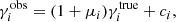
To start, we explore the accuracy of the KSB correction for PSF anisotropy. To quantify the bias, we introduce the smear polarisability boost factor, $b_i^{\text{sm}}$, by which we multiply the KSB estimate to ensure a vanishing additive bias caused by PSF anisotropy. As an example, we consider a galaxy with a surface brightness profile defined by Sérsic-parameter n and an effective radius of $r_{\mathrm{eff}}=0\stackrel{″}{.}3$ (a typical size for sources used in cosmic shear studies). We consider two PSFs: our approximation to the Euclid PSF (described in Sect. 3), and a Gaussian PSF with FWHM = $0\stackrel{″}{.}2$. In both cases we use ${ϵ}_i^{\mathrm{PSF}}=0.1$ for the PSF ellipticity.

Equation (5) implies that P^sm = 1 for a point source. In the KSB formalism this is ensured by dividing the observed smear polarisability of a galaxy by that measured for the PSF. We multiply this estimate by $b_i^{\text{sm}}$ so that the corrected polarisation vanishes. For both PSFs, we find that $b_i^{\text{sm}}$ depends on the galaxy ellipticity, but as we are mainly interested in ensembles of galaxies, we show the resulting $\langle b_i^{\text{sm}}\rangle$ as a function of the Sérsic-parameter n of the galaxy in Fig. 1 (with the galaxy ellipticities sampled uniformly between −0.5 < ϵ_i < 0.5).

Fig. 1. Smear polarisability boost factor, $b_i^{\text{sm}}$ as a function of Sérsic n for a galaxy with an effective radius of $0\stackrel{″}{.}3$. The Gaussian PSF has a FWHM of $0\stackrel{″}{.}2$ and the Airy PSF is our Euclid-like PSF (see Sect. 3). The shaded regions indicate the variation in $b_i^{\text{sm}}$ when the PSF size is varied by ±10%. The sensitivity to the PSF size is negligible for ${\sigma }_{\mathrm{w}}=0\stackrel{″}{.}3$ in this case, whereas $b_i^{\text{sm}}\approx 1$ for the Gaussian PSF.

In the case of a Gaussian PSF, the average value of $b_i^{\text{sm}}$ does not depend on n. For ${\sigma }_{\mathrm{w}}=0\stackrel{″}{.}2$ we find $\langle b_i^{\text{sm}}\rangle$ = 1.005, and for ${\sigma }_{\mathrm{w}}=0\stackrel{″}{.}3$ the value is consistent with 1; the KSB correction works well for a Gaussian PSF. The situation is markedly different for the Airy PSF, with a strong dependence of $b_i^{\text{sm}}$ on the galaxy surface brightness profile, whilst it also depends on the PSF size. The shaded regions in Fig. 1 indicate the range in $b_i^{\text{sm}}$ if the PSF size is changed by ±10%. For the larger weight function, which is better matched to the galaxy size, the sensitivity is negligible, but for the smaller value of ${\sigma }_{\mathrm{w}}=0\stackrel{″}{.}2$, $b_i^{\text{sm}}$ also depends somewhat on PSF size. We explored this a little bit further and found that a weight function that matches the galaxy size may result in reduced sensitivity to the PSF size. We do not pursue this further here, but leave this for future study. Instead, we follow H21 and use a fixed width.

Figure 1 shows that KSB can only accurately correct for PSF anisotropy if the PSF is Gaussian. For more realistic PSF profiles, the correction needs to be boosted by a factor of $b_i^{\text{sm}}$. The value of $b_i^{\text{sm}}$ depends on the PSF and galaxy profiles, as well as the weight function. The correction, however, can be determined empirically by requiring that the additive shear bias vanishes for any particular subset of galaxies. This assumes that PSF anisotropy is the only source of additive shear bias. Although this is a reasonable approximation, residual detector effects, such as charge transfer inefficiency (e.g., Massey et al. 2014) or charge trailing, can also contribute. We do not consider these complications here, as they are typically subdominant.

That leaves the determination of the multiplicative bias, for which we want to use METADETECTION, which was introduced by Sheldon et al. (2020) as a data-driven approach to estimate shear, whilst accounting for selection biases. As shown in H21, it yields unbiased shear estimates that meet Euclid requirements in the absence of PSF anisotropy. In principle, it can also account for PSF anistropy, but this involves additional, expensive, image manipulations, whilst degrading the image quality. Avoiding this, if possible, led to our hybrid approach. The key question now is whether correcting the polarisations for PSF anisotropy biases the estimation of the multiplicative shear bias.

We refer the interested reader to the original papers that describe the methodology. Here, we only provide the salient points. The starting point of METADETECTION is the creation of sheared images from which the response to an applied shear can be inferred. This procedure is described in detail in Huff & Mandelbaum (2017) and Sheldon & Huff (2017), who refer to this as METACALIBRATION. The only assumption of METACALIBRATION is that we can construct a sheared version, I^sh(x|γ) of the true image using the observed image I(x) via Eq. (5) of Huff & Mandelbaum (2017):

$$\begin{array}{c}\hfill I^{\mathrm{sh}}(\mathit{x}|\mathit{\gamma })=P(\mathit{x})\ast [{\widehat{s}}_{\gamma }\{P{(\mathit{x})}^{-1}\ast I(\mathit{x})\}],\end{array}$$(6)

where ${\widehat{s}}_{\gamma }$ is the shear operator (Bernstein & Jarvis 2002), P(x) is the PSF, I(x) the observed image, and ‘*’ indicates convolution. Hence, the observed image is first deconvolved (P(x)⁻¹ * I(x)), then sheared by ${\widehat{s}}_{\gamma }$, and finally re-convolved by the PSF. In practice, noise in the data complicates the deconvolution step, and a slightly larger PSF is needed to suppress the noise. The modified PSF, P^meta(x), to use in the reconvolution step in Eq. (6) is (Huff & Mandelbaum 2017)

$$\begin{array}{c}\hfill P^{\mathrm{meta}}(\mathit{x})=P(\mathit{x}/(1+2|\gamma |)).\end{array}$$(7)

The shearing of the images leads to anisotropic correlated noise, which can be accounted for by adding anisotropic noise (Sheldon & Huff 2017). This results in a slight increase in the overall noise level, which is of little concern.

The response of the polarisation of a galaxy to an applied shear, γ, can be obtained by using Eq. (6) and measuring χ and comparing it to χ_γ = 0, the unsheared case:

$$\begin{array}{c}\hfill {\chi \approx \chi |}_{\gamma =0}+\frac{\partial \chi }{\partial \gamma }{|}_{\gamma =0}{\gamma \equiv \chi |}_{\gamma =0}+{\mathsf{R}}^{\gamma }\gamma ,\end{array}$$(8)

where R^γ is the 2 × 2 shear response tensor. Its elements can be estimated by measuring the shapes of the galaxies in the sheared images and computing

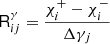$$\begin{array}{c}\hfill {\mathsf{R}}_{\mathit{ij}}^{\gamma }=\frac{{\chi }_i^{+}-{\chi }_i^{-}}{\mathrm{\Delta }{\gamma }_j}\end{array}$$(9)

where the subscripts indicate the two shear components, and the superscript the sign of the applied shear, so that ‘+’ means the image was sheared by +γ_j, etc; hence, Δγ_j = 2γ_j. The measurement of the shear response is determined more precisely for larger values of Δγ, but larger values can also lead to a bias from higher-order contributions (Sheldon & Huff 2017). H21 compared results for Δγ = 0.01 and Δγ = 0.02, and found that the latter performed somewhat better. We therefore use this value throughout this paper as well.

These expressions are true for any shape measurement, but do implicitly assume that the images are sampled well. This potential limitation was studied in detail by Kannawadi et al. (2021), who showed that employing a sufficiently large weight function can effectively eliminate any bias arising from poorly sampled images. The weight functions we used here avoid this problem (our baseline uses ${\sigma }_{\mathrm{w}}=0\stackrel{″}{.}2$), as is supported by the small biases obtained by H21.

We estimated the shear, $\widehat{\gamma }$ for an ensemble of galaxies using

$$\begin{array}{c}\hfill \widehat{\gamma }\approx {⟨{\mathsf{R}}^{\gamma }⟩}^{-1}⟨\chi ⟩={⟨{\mathsf{R}}^{\gamma }⟩}^{-1}⟨{\mathsf{R}}^{\gamma }\gamma ⟩,\end{array}$$(10)

that is, we averaged the estimates for the shapes and the shear responses, rather than using estimates per galaxy. The reason is that the estimates for R^γ are very noisy for individual galaxies, and averaging reduces biases in the shear estimate, which formally requires the inverse of R^γ. Moreover, we found that both diagonal elements are consistent with one another, so that we can simply approximate R^γ by a scalar.

Although METACALIBRATION yields unbiased shear estimates for the detected galaxies, the final shear estimate suffers from detection bias. To account for this Sheldon et al. (2020) proposed METADETECTION which uses the same images, but both the detection and the shape analysis are performed on these images. By avoiding the use of the unsheared image as a reference, the detection bias vanishes, as was demonstrated in H21.

3. Simulated data

We tested the performance of our shape measurement algorithm using simulated data. Our baseline setup is identical to that used in H21, which in turn was based on Hoekstra et al. (2017); the only difference is the use of an anisotropic PSF. We refer the interested reader to these two papers for more details and tests, because here we provide a minimal description.

The surface brightness profiles of the galaxies are described by Sérsic profiles, with half-light radii, apparent magnitudes and Sérsic indices n drawn from a catalogue of morphological parameters measured from resolved F606W images from the GEMS survey (Rix et al. 2004). We only considered galaxies fainter than magnitude m = 20 and used the morphological parameters from the GEMS catalogue for galaxies down to m = 25.4, and normalised the counts to 36 galaxies arcmin⁻² with 20 < m < 24.5. We include fainter galaxies (down to m = 29) as described in Hoekstra et al. (2017) and H21. The intrinsic ellipticities were drawn from a Rayleigh distribution with scale parameter ϵ₀ = 0.25, so that the mean source ellipticity is ⟨|ϵ^s|⟩ ≈ 0.31.

In our baseline simulations we placed galaxies randomly, but with random sub-pixel offsets. Although the clustering of faint satellite galaxies around their host galaxies is important (Euclid Collaboration 2019), ignoring this complication does not affect our main results, because METADETECTION accounts for blending (see H21 and Sect. 4.2). For a number of tests we also created images where the galaxies were placed on a grid, so that they are about 9″ apart, thus eliminating any blending. This provided a useful reference to compare our baseline results against. To reduce shape noise, we created pairs of images, where the galaxies were placed at the same location, but rotated by 90 degrees in the rotated case. We used SEXTRACTOR (Bertin & Arnouts 1996) to detect objects in the simulated images.

In Sect. 4 we present results for our Euclid-like data, which can be compared directly to the findings of H21. We approximate the Euclid PSF in the VIS-band (Cropper et al. 2018) by adopting an Airy profile for a telescope with a diameter of 1.2 m and an obscuration of 0.3 at a reference wavelength of 800 nm. The PSF anisotropy was introduced by shearing the circular PSF profile by ${ϵ}_i^{\text{PSF}}$. To create the images for the METADETECTION step we used a 5× oversampled PSF image; this image was also used for the estimation of the KSB PSF correction parameters.

The simulated images were created using the publicly available software package GALSIM⁶ (Rowe et al. 2015). The individual images are 4000 pixels on a side, with a pixel size of $0\stackrel{″}{.}1$ per pixel. The noise level corresponds to a surface brightness of 27.7 magnitudes arcsecond⁻². This mimics the depth of four coadded Euclid exposures, and yields a typical number density of 47 galaxies arcmin⁻² with a signal-to-noise ratio larger than 10, as measured by SEXTRACTOR(Bertin & Arnouts 1996), and a number density of 33 galaxies arcmin⁻² if we restrict the magnitude range to 20 < m < 24.5.

In Sect. 5 we examine the performance for ground-based observations. In this case the PSF is described by a Moffat profile (Moffat 1969) with a FWHM = $0\stackrel{″}{.}7$ and β = 2. Those images have a pixel size of $0\stackrel{″}{.}2$ and a noise level corresponding to a surface brightness of 28.1 magnitudes arcsecond⁻², or equivalently a 10σ point source detection limit of about 26.5, similar to the depth of LSST after ten years of operations.

4. Airy PSF

In this section we present results for an anisotropic Euclid-like PSF. Our study ignores many real-life complications, such as those arising from a wavelength-dependent PSF and a broad pass-band (Semboloni et al. 2013; Er et al. 2018; Eriksen & Hoekstra 2018).We implicitly assume that it is possible to derive an accurate PSF for each galaxy.

We used the METACALIBRATION routines (Sheldon & Huff 2017) to create the sheared images, detected objects using SEXTRACTOR (Bertin & Arnouts 1996), and measured the polarisations of the galaxies. Unless specified otherwise, the polarisations were measured using a Gaussian weight function with ${\sigma }_{\mathrm{w}}=0\stackrel{″}{.}2$. We verified that similar results were obtained using ${\sigma }_{\mathrm{w}}=0\stackrel{″}{.}3$, confirming that the accuracy of METADETECTION does not depend critically on the choice of weight function.

4.1. Grid-based simulation

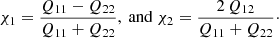
Before considering more realistic scenarios, we start with a more ideal setup, with galaxies placed on a grid. This minimised the complications introduced by blending. The galaxies in the simulated images differed only by the PSF ellipticity that was used, resulting in (some) correlated shape noise for the measurements presented here.

The orange points in Fig. 2 show the multiplicative bias (top panel) and additive bias (bottom panel) for galaxies with 20 < m_VIS < 24.5 if the observed polarisations are not corrected for PSF anisotropy. The error bars reflect the number of simulated images. Not surprisingly, the additive biases are very large, about 30% of ϵ^PSF, but the multiplicative bias after METADETECTION is consistent with zero, even if the PSF is highly elliptical. Correcting the polarisations using the KSB estimate for the smear polarisability ($b_i^{\text{sm}}=1$) reduces the additive bias by a factor of 5.6 (red points in Fig. 2).

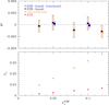Fig. 2. Multiplicative bias, μ (top) and additive bias, ci (bottom) after METADETECTION, as a function of PSF ellipticity, ${ϵ}_i^{\text{PSF}}$, for galaxies with 20 < mVIS < 24.5 that were placed on a grid. The orange points correspond to the results without correction for PSF anisotropy, whereas the red points indicate the biases after the nominal KSB correction (bsm = 1). The black points show the results using the value for bsm that nulls the additive bias for the grid-based simulations, whereas the blue squares correspond to our baseline setup, where galaxies were placed randomly (see Sect. 4.2; in this case the error bars are smaller, because we simulated more images for the baseline case). We do not show the corresponding additive biases, because those are consistent with zero by construction.

It is worthwhile to contrast the residual additive biases to the Euclid requirements. The breakdown presented in Cropper et al. (2013) suggests that the total additive shear bias should be |c|< 1.3 × 10⁻⁴. This also includes contributions from errors in the PSF model and residual biases caused by detector effects, in particular charge transfer inefficiency (Massey et al. 2014). The allocation for additive bias caused by the shape measurement algorithm implies |c_i|< 5.2 × 10⁻⁵, which is truly challenging⁷. We do note that this requirement is actually conservative, because the PSF varies across the survey, reducing the net additive bias on larger scales. As shown in Kitching et al. (2019), the approach used by Cropper et al. (2013) is not well suited for spatially varying biases. Although these papers provided a good starting point to derive requirements, once the instrument design has been established, it is better to propagate biases forward in a consistent manner, as was done in Euclid Collaboration (2020). Regardless, it is clear that using KSB to correct for PSF anisotropy yields additive biases that exceed the Euclid requirements by orders of magnitude.

Interestingly, regardless of whether the polarisations are corrected for PSF anisotropy, the corresponding multiplicative biases are consistent with zero. This suggests that the correction for multiplicative and (residual) additive bias can be determined separately, with METADETECTION yielding negligible multiplicative bias, whilst any residual PSF anisotropy can be accounted for empirically. For instance, one could simply adopt $b_i^{\mathrm{sm}}=P_{\mathit{ii}}^{\mathrm{sm}}$, thus ignoring the KSB estimate for the smear polarisability. We do not advocate this, because the ‘raw’ corrections for PSF anisotropy are large and depend strongly on the galaxy and PSF properties. Instead, we started with the KSB estimate for the smear polarisability. This should result in a more robust empirical correction because the KSB estimate captures most of the variation with galaxy properties, at minimal computational cost.

We multiplied the KSB smear polarisabilities for a particular (sub)sample of galaxies with a boost factor and computed the average additive bias after correction for PSF anisotropy. The residual additive bias depends linearly on the boost factor, and we defined $b_i^{\text{sm}}$ as the boost factor for which the mean residual additive bias vanished. The black points in the top panel of Fig. 2 show the resulting multiplicative biases as a function of PSF ellipticity. We do not show the residual additive biases, as they vanish by construction.

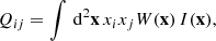
We did not explore the full range in sensitivities here, but as an example, Fig. 3 shows that $b_i^{\text{sm}}$ varies quadratically with increasing PSF ellipticity. The resulting multiplicative biases are indicated by the black points in the top panel of Fig. 2. The dependence with ϵ_PSF is reduced by a factor of 4.4 if we use a larger weight function (bottom panel of Fig. 3). The boost factors are consistent for both shear components. We observed this in all subsequent results, and we therefore use the average of both components, b^sm, in the remainder of the paper.

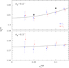Fig. 3. Correction factor $b_i^{\text{sm}}$ as a function of PSF ellipticity for a weight function ${\sigma }_{\mathrm{w}}=0\stackrel{″}{.}2$ (top) and ${\sigma }_{\mathrm{w}}=0\stackrel{″}{.}3$ (bottom). The red and blue points show the results for the individual shear components using the grid-based simulations. The lines are the best-fit model (see text) to both components jointly. The bias is smaller overall for the larger weight function, whilst the dependence with PSF ellipticity is also reduced. The black squares in the top panel correspond to our baseline setup, with galaxies placed randomly. This suggests that blending has a small impact on the correction.

4.2. Baseline simulations

As shown in H21 blending is an important source of bias. We therefore proceed with a more realistic setup, where galaxies are placed randomly. H21 already showed that in this case METADETECTION can recover the shear signal if the PSF is round. Here, we examine if this is still the case for an anisotropic PSF. We used ${\sigma }_{\mathrm{w}}=0\stackrel{″}{.}2$, so that the results can be compared directly to those presented in H21 for a round PSF.

As was the case for the grid-based simulations, the values for $b_i^{\text{sm}}$ are consistent for both components, and thus can be averaged. We show the averaged results in the top panel of Fig. 3 as black points, which are slightly higher than those obtained for the grid-based simulations. This suggests that the level of blending affects the correction, something we return to in Sect. 4.2. The resulting multiplicative biases are shown in blue in Fig. 2, and are consistent with zero. The smaller error bars reflect the larger number of images simulated for the baseline case.

Thus far, we have only considered average biases for the full population of galaxies with 20 < m_VIS < 24.5, but we expect some dependence with size and magnitude. This is explored in Fig. 4. The additive bias (middle panels) increases for fainter, smaller galaxies, as expected. The correction to the KSB smear polarisability also depends on magnitude and observed size, as shown in the bottom panels, but the dependence is smooth. The multiplicative biases, however, are small, even if we do not correct for PSF anisotropy.

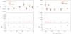Fig. 4. Left panel: residual multiplicative bias (top), additive bias (middle) and estimate for bsm (bottom) as a function of observed magnitude, mAUTO, determined by SEXTRACTOR. Right panel: idem, but as a function of the observed half-light radius, $r_h^{\mathrm{obs}}$. The orange points indicate the biases when the polarisations are not corrected for PSF anisotropy, whereas the red points are for the standard KSB correction. The black points use bsm to correct for PSF anistropy, resulting in vanishing additive bias by construction (and therefore not shown).

The estimates for both the polarisation and the polarisabilities depend on ratios of moments. In the presence of noise, such ratios are biased (e.g., Viola et al. 2014), and thus we may expect that b^sm is sensitive to the noise level. This is explored in Fig. 5, where we multiply the noise level by a factor of f_noise with respect to the baseline case. The results are shown for ϵ_PSF = 0.1. The figure shows that the multiplicative bias after METADETECTION for galaxies with 20 < m_VIS < 24.5 does not depend on the noise level, but that the best estimate for b^sm does. If instead we use the value for the baseline setup, the resulting residual additive biases exceed the Euclid requirements.

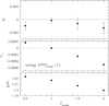Fig. 5. Top panel: multiplicative bias after METADETECTION for galaxies with 20 < mVIS < 24.5 when the noise is increased by a factor of fnoise with respect to the baseline case, with ϵPSF = 0.1. Middle panel: residual multiplicative bias ci if we use bsm = 1.217, the estimate for the baseline case. Bottom panel: best estimate for bsm as a function of fnoise, which shows a clear dependence on the noise level. If ignored, the residual multiplicative biases exceeds Euclid requirements for this level of PSF anisotropy.

To ensure a vanishing additive shear bias, it is thus necessary to account for the sensitivity to the noise level. Also, the dependence of b^sm with flux (or signal-to-noise ratio) and size needs to be modelled. These dependences, however, can be inferred from the data, which is markedly different from the empirical corrections based on image simulations that are currently employed (Hoekstra et al. 2015; Fenech Conti et al. 2017; Kannawadi et al. 2019). Moreover, the behaviour of b^sm appears to be smooth, and the variation rather small, suggesting that this can be fitted with a low-order function. Alternatively, machine learning approaches can be used to model b^sm, as a function of observed properties (which may include any variation in PSF size). This would be far more efficient (and effective) than current attempts that aim to learn the mapping between data and shear directly using simulated data (e.g., Tewes et al. 2019).

The advantage of our method is that it is completely data-driven. It does rely on an accurate model of the PSF, but this applies to any shape measurement algorithm. The only other assumption we have made is that the PSF anisotropy is the dominant source of additive bias. This may not always be the case, as imperfections in the detector or the read-out electronics can cause charge to trail. Although our approach would still ensure that the additive bias vanishes, the multiplicative bias may not. For instance, Appendix B in H21 shows how trailing introduces comparable additive and multiplicative biases. Either additional sources of biases have to be corrected for before the METADETECTION process or their impact needs to be simulated to determine empirical corrections.

The validity of the assumptions can be tested by comparing the estimates for b^sm to those determined from realistic image simulations. Any deviations would either point to issues with the simulated data or indicate the presence of additional sources of additive bias. This changes the role of the simulations for shear calibration: rather than using them to calibrate the algorithm (which still is an option), the simulations are used to validate the correction. As a further sophistication, b^sm could be determined as a function of galaxy polarisation in the frame defined by the PSF orientation. However, as cosmic shear surveys average large ensembles of galaxies, ignoring this only slightly increases the effective shape noise.

Figure 2 shows that the estimate for b^sm is slightly higher when galaxies are placed randomly, suggesting that blending plays a role. Indeed, H21 showed that blending is an important source of shear bias, which is exacerbated by the clustering of galaxies (Euclid Collaboration 2019). Although we ignore clustering here, we quantify how variations in the galaxy density affect the performance of our algorithm.

The left panel in Fig. 6 shows the residual multiplicative and additive bias for galaxies with 20 < m_VIS < 24.5 as a function of r_sep, the distance to the nearest galaxy in the input catalogue. Both the multiplicative bias and additive bias are consistent with zero. As a further test we vary the overall level of blending by increasing the number density of galaxies in the simulations by a factor of n_fac, where n_fac = 0 corresponds to the grid-based case. The results are presented in the right panel of Fig. 6. We find that the multiplicative bias is consistent with zero. The value of b^sm does depend on n_fac (bottom panel), but we ignored this, and used the value for the fiducial to obtain the additive biases shown in the right panel of Fig. 6. The results are very encouraging, because even for n_fac = 2, which approaches the mean galaxy density in clusters, the residual additive bias is small. Although the additive bias exceeds the Euclid requirement for extreme values of n_fac, variations in galaxy density are generally far less extreme, and will tend to average out.

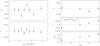Fig. 6. Left panel: residual multiplicative bias (top) and additive bias (bottom) as a function of rsep, the distance to the nearest galaxy in the input catalogue brighter than m = 26. Right panel: residual biases as a function of nfac, the relative increase in galaxy density, where nfac corresponds to the grid-based case. In both cases, results were obtained using bsm = 1.217, the best estimate for the fiducial setup. The results indicate that the performance is not affected significantly by blending, although the additive biases exceed Euclid requirements for extreme over- and under-densities.

4.3. PSF modelling errors

Our empirical correction cannot distinguish between an error in the PSF model and a bias in the correction for PSF anisotropy. Instead, the empirical estimate for b^sm will be biased with respect to the value corresponding to the actual PSF. Nonetheless, the low sensitivity of METADETECTION to the PSF anisotropy suggests that the multiplicative bias may not be affected much by errors in the model PSF ellipticity. If true, this opens up alternative approaches to account for coherent patterns in the residual PSF ellipticity.

In this section we therefore explore the sensitivity to PSF modelling errors. We consider errors in the PSF size and the PSF ellipticity, but examine these separately. Depending on how the PSF is modelled, these may be correlated in practice. We analysed images with ${ϵ}_i^{\text{PSF}}$ = 0.1, but used a biased PSF in the correction. Because the input images are unchanged, we used METACALIBRATION, as changes in the detection bias should be minimal (we verified that METADETECTION yields a consistent result for an extreme case). To correct for PSF anisotropy, we used the value of b^sm for the correct PSF (otherwise the additive bias would have vanished). The results thus capture the impact of variations in PSF error across the survey.

The results are presented in Fig. 7. The left panels show the change in multiplicative bias (top) and additive bias (bottom) as a function of Δ${ϵ}_i^{\text{PSF}}$, the error in PSF ellipticity. The multiplicative bias changes somewhat as well, because the (extra) shearing of the PSF also changes the size, quantified by $R_{\text{PSF}}^2=P_{11}+P_{22}$. We approximate the unweighted PSF quadrupole moments by those using a weight function with ${\sigma }_{\mathrm{w}}=0\stackrel{″}{.}75$, but note that this choice does not matter much for the relative change in size, $\mathrm{\Delta }{R}_{\text{PSF}}^2/R_{\text{PSF}}^2$. The right panels in Fig. 7 show the results when the PSF ellipticity is fixed, but the size of the PSF is changed isotropically. Not surprisingly, the multiplicative bias changes the most, but the incorrect PSF size also introduces some PSF anisotropy.

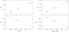Fig. 7. Left: change in multiplicative bias (top) and additive bias (bottom) as a function of Δ${ϵ}_i^{\text{PSF}}$, the error in PSF ellipticity. Right: idem, but when the size of the PSF is changed isotropically. The relative change in size is quantified by $\mathrm{\Delta }{R}_{\text{PSF}}^2/R_{\text{PSF}}^2$, computed using the PSF quadrupole moments. In both cases, the multiplicative and additive biases increase linearly with the PSF error, but we note the different scales: The multiplicative bias is more sensitive to size errors, whereas the additive bias is most sensitive to errors in the PSF ellipticity.

Cropper et al. (2013) allocated |c|< 7.6 × 10⁻⁵ for the additive bias caused by the error in the PSF ellipticity. Based on our findings, this implies |Δϵ_PSF|< 2.5 × 10⁻⁴, whilst the corresponding change in multiplicative bias is negligible (|Δμ|< 3 × 10⁻⁵). Our inferred tolerance on the PSF ellipticity error is about a factor of two less stringent⁸. Similarly the allocation for the multiplicative bias caused by errors in the PSF size of |Δμ|< 3 × 10⁻⁴ implies that 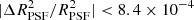$|\mathrm{\Delta }{R}_{\text{PSF}}^2/R_{\text{PSF}}^2|<8.4\times {10}^{-4}$, also close to the estimate from Cropper et al. (2013). The analytical estimates are thus fairly accurate for our Euclid-like PSF.

At first glance, there seems little room to relax the accuracy with which both PSF ellipticity and size need to be determined. It is, however, useful to distinguish between global and spatially varying residuals, something that was not done by Cropper et al. (2013). Although it is challenging to ensure a mean PSF error that meets requirements, it is even more difficult to achieve at any point in the survey. We should, however, consider the impact of spatially varying errors in the PSF size and PSF ellipticity separately. The latter directly contribute to the shear power spectrum, because neighbouring galaxies share a common PSF modelling error, whilst introducing a small spatially varying multiplicative bias as well. If the errors in PSF size are small and average out across the survey, they should not bias the cosmological analysis (Kitching et al. 2019).

The main concern is therefore the impact of the residual additive bias arising from PSF modelling errors. Although we do not advocate relaxing the requirements with which the PSF model needs to be determined, we do note that a coherent pattern of PSF residuals can be accounted for empirically. For instance, one could average the shear estimates from many images in the frame defined by the focal plane. Ignoring detector effects that can also contribute, any residual pattern would then be the result of a coherent error in the PSF model. The contribution of this pattern to the shear power spectrum can then be estimated, and be accounted for in the cosmological analysis.

A vanishing mean additive bias is, however, not sufficient. For instance, random errors in the focus will flip the sign of the error in PSF ellipticity, but the corresponding additive biases still affect the shear power spectrum. This is captured by the power spectrum of the residual PSF ellipticies (Hoekstra 2004), and could be included in the cosmological analysis, as its power spectrum typically will be different from the cosmological signal. Such an analysis would not pick up the contribution to the additive bias caused by errors in PSF size. One could attempt to determine those directly, but this is far more difficult than measuring shapes. Avoiding this requires either low PSF anisotropy or accurate modelling of the PSF size itself. In the end, the best strategy is therefore to use the available information to improve the PSF model itself. Moreover, the best way to estimate the implications for cosmological parameter estimates is to simulate the impact of residual errors on the analysis (e.g., Euclid Collaboration 2020).

5. Moffat PSF

Thus far we have focused on observations that mimic Euclid data. To explore the viability of our approach for ground-based observations we created images using a Moffat profile (Moffat 1969), with β = 2 and a FWHM = $0\stackrel{″}{.}7$, a pixel scale of $0\stackrel{″}{.}2$, and a sky background noise level of 28.1 mag arcsec⁻², comparable to the depth reached by LSST after ten years of operations. The input catalogue is the same as before, and the galaxies were placed randomly. To measure the shapes, we used ${\sigma }_{\mathrm{w}}=0\stackrel{″}{.}6$.

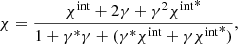
As shown in Fig. 8, the resulting additive bias is larger, because of the larger PSF. Compared to the Euclid-like PSF, the KSB correction performs better in a relative sense: the additive bias is reduced by a factor of 8.2 for the Moffat profile. Importantly, the recovered multiplicative biases are consistent with zero, even for the very elliptical PSFs we used.

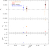Fig. 8. Top panel: multiplicative bias of galaxies with 20 < mr < 24.5 after METADETECTION for simulated ground-based observations with a PSF that follows a Moffat profile with FWHM = $0\stackrel{″}{.}7$. Middle panel: residual additive bias ci if we do not correct the polarisations (orange) or use the standard KSB correction (red). Bottom panel: best estimate for bsm as a function of ${ϵ}_i^{\text{PSF}}$. The blue points shows the results for a double Moffat profile with a large ellipticity gradient (see Sect. 5 for details). Also for this more complex PSF do we find a multiplicative bias that is consistent with zero.

The PSFs considered thus far have minimal ellipticity gradients; the only gradient is introduced by the pixelation, which makes the central part of the PSF somewhat rounder. The PSF ellipticity, however, may vary with radius (Hoekstra et al. 1998). Our empirical correction should still work, but for completeness we examine the impact here using a ground-based PSF with a strong ellipticity gradient.

The PSF is constructed to have the same unweighted ‘size’, R², as the single ellipticity PSF used in the previous section. The core of the more complex PSF is described by a Moffat profile with a FWHM that is 0.8 times the original PSF, and it contains 70% of the flux. Here, we consider only ${ϵ}_i^{\text{PSF}}$ = 0.1. To this central PSF, we add another Moffat profile, with the same ellipticity, but at an angle of 90° to maximise the ellipticity gradient. Its FWHM is 1.4 times the original PSF, and it contains 30% of the flux. The unweighted ellipticity of this PSF is about −0.004, that is almost round. More relevant is the ellipticity determined using the typical observed size of the galaxies, which yields an effective ellipticity of 0.041. We used this value to plot the results in Fig. 8. Other than changing the PSF, the analysis is the same as before.

The results are presented in Fig. 8 as blue points. The value for b^sm is lower, but the residual additive biases are in line with the expectations for the effective PSF ellipticity. The light blue point ignores the PSF anisotropy altogether, whereas the bias after the KSB correction (dark blue point) is a factor of 5.6 lower. Consistent with the findings of Hoekstra et al. (1998), KSB performs also reasonably well for complex PSFs. The multiplicative bias is consistent with zero (we show only the result for the best estimate of b^sm as the dark blue point). This demonstrates that our data-driven correction also performs well for a PSF with a strong ellipticity gradient.

6. Conclusions

Algorithms to determine the shear from images need to accurately correct for multiplicative and additive bias introduced by the PSF. We studied the prospects of a fully data-driven approach, based on METADETECTION (Sheldon et al. 2020), which is able to yield unbiased shear estimates in the absence of PSF anisotropy. We focused on the performance for Euclid-like data, extending the earlier work by H21 to data with significant PSF anisotropy, but also presented results for a ground-based case, including a PSF with a strong ellipticity gradient.

We found that the multiplicative bias after METADETECTION is consistent with zero, whilst being nearly insensitive to the PSF anisotropy. We exploited this finding and showed how the resulting additive bias can be removed using the data themselves, under the assumption that the PSF anisotropy is the sole source of additive bias. Although METADETECTION itself can also be used to estimate the sensitivity of the shape measurement to PSF anisotropy, it requires additional, relatively costly, computations. Instead, he we explored the viability of correcting the observed shape estimates first.

To do so, we started by correcting the observed shapes for PSF anisotropy using the estimate for the smear polarisability derived by Kaiser et al. (1995). This reduced the additive bias, but the residuals were too large for cosmic shear studies. To improve the correction we boosted the smear polarisability by a factor of b^sm, whose value is determined empirically by requiring that the additive bias vanishes. The value of b^sm depends on the usual parameters that affect the performance of shape measurements, but it varies smoothly, and thus is easily modelled. Although our approach is fully data-driven, b^sm could also be determined using simulated data instead. Comparison with the observed estimates might highlight issues with either the data or the simulations.

Further optimisation is possible. Our baseline results employed a fixed weight function with ${\sigma }_{\mathrm{w}}=0\stackrel{″}{.}2$, which resulted in a small dependence of b^sm with PSF ellipticity, and a sensitivity on the PSF size. Using a broader weight function reduces the sensitivity to both. In particular, matching the weight function to the size of the galaxy may reduce the overall sensitivity of b^sm, although a minimum size may be required for poorly sampled data (Kannawadi et al. 2021). Moreover, the best estimate for b^sm depends on the polarisation of the galaxy with respect to the PSF anisotropy. This dependence could be explicitly included, thus improving the accuracy of the correction for individual galaxies. Such more complex corrections are well suited for machine learning approaches.

Acknowledgments

The author thanks Hendrik Hildebrandt, Arun Kannawadi, Tom Kitching and Tim Schrabback for suggestions that improved the paper. The author is also grateful to Erin Sheldon and the developers of GALSIM for making their software packages publicly available. The author acknowledges support from the Netherlands Organisation for Scientific Research (NWO) through grant 639.043.512 and from the EU Horizon 2020 research and innovation programme under grant agreement 776247.

References

All Figures

Fig. 1. Smear polarisability boost factor, $b_i^{\text{sm}}$ as a function of Sérsic n for a galaxy with an effective radius of $0\stackrel{″}{.}3$. The Gaussian PSF has a FWHM of $0\stackrel{″}{.}2$ and the Airy PSF is our Euclid-like PSF (see Sect. 3). The shaded regions indicate the variation in $b_i^{\text{sm}}$ when the PSF size is varied by ±10%. The sensitivity to the PSF size is negligible for ${\sigma }_{\mathrm{w}}=0\stackrel{″}{.}3$ in this case, whereas $b_i^{\text{sm}}\approx 1$ for the Gaussian PSF.

In the text

Fig. 2. Multiplicative bias, μ (top) and additive bias, ci (bottom) after METADETECTION, as a function of PSF ellipticity, ${ϵ}_i^{\text{PSF}}$, for galaxies with 20 < mVIS < 24.5 that were placed on a grid. The orange points correspond to the results without correction for PSF anisotropy, whereas the red points indicate the biases after the nominal KSB correction (bsm = 1). The black points show the results using the value for bsm that nulls the additive bias for the grid-based simulations, whereas the blue squares correspond to our baseline setup, where galaxies were placed randomly (see Sect. 4.2; in this case the error bars are smaller, because we simulated more images for the baseline case). We do not show the corresponding additive biases, because those are consistent with zero by construction.

In the text

Fig. 3. Correction factor $b_i^{\text{sm}}$ as a function of PSF ellipticity for a weight function ${\sigma }_{\mathrm{w}}=0\stackrel{″}{.}2$ (top) and ${\sigma }_{\mathrm{w}}=0\stackrel{″}{.}3$ (bottom). The red and blue points show the results for the individual shear components using the grid-based simulations. The lines are the best-fit model (see text) to both components jointly. The bias is smaller overall for the larger weight function, whilst the dependence with PSF ellipticity is also reduced. The black squares in the top panel correspond to our baseline setup, with galaxies placed randomly. This suggests that blending has a small impact on the correction.

In the text

Fig. 4. Left panel: residual multiplicative bias (top), additive bias (middle) and estimate for bsm (bottom) as a function of observed magnitude, mAUTO, determined by SEXTRACTOR. Right panel: idem, but as a function of the observed half-light radius, $r_h^{\mathrm{obs}}$. The orange points indicate the biases when the polarisations are not corrected for PSF anisotropy, whereas the red points are for the standard KSB correction. The black points use bsm to correct for PSF anistropy, resulting in vanishing additive bias by construction (and therefore not shown).

In the text

Fig. 5. Top panel: multiplicative bias after METADETECTION for galaxies with 20 < mVIS < 24.5 when the noise is increased by a factor of fnoise with respect to the baseline case, with ϵPSF = 0.1. Middle panel: residual multiplicative bias ci if we use bsm = 1.217, the estimate for the baseline case. Bottom panel: best estimate for bsm as a function of fnoise, which shows a clear dependence on the noise level. If ignored, the residual multiplicative biases exceeds Euclid requirements for this level of PSF anisotropy.

In the text

Fig. 6. Left panel: residual multiplicative bias (top) and additive bias (bottom) as a function of rsep, the distance to the nearest galaxy in the input catalogue brighter than m = 26. Right panel: residual biases as a function of nfac, the relative increase in galaxy density, where nfac corresponds to the grid-based case. In both cases, results were obtained using bsm = 1.217, the best estimate for the fiducial setup. The results indicate that the performance is not affected significantly by blending, although the additive biases exceed Euclid requirements for extreme over- and under-densities.

In the text

Fig. 7. Left: change in multiplicative bias (top) and additive bias (bottom) as a function of Δ${ϵ}_i^{\text{PSF}}$, the error in PSF ellipticity. Right: idem, but when the size of the PSF is changed isotropically. The relative change in size is quantified by $\mathrm{\Delta }{R}_{\text{PSF}}^2/R_{\text{PSF}}^2$, computed using the PSF quadrupole moments. In both cases, the multiplicative and additive biases increase linearly with the PSF error, but we note the different scales: The multiplicative bias is more sensitive to size errors, whereas the additive bias is most sensitive to errors in the PSF ellipticity.

In the text

Fig. 8. Top panel: multiplicative bias of galaxies with 20 < mr < 24.5 after METADETECTION for simulated ground-based observations with a PSF that follows a Moffat profile with FWHM = $0\stackrel{″}{.}7$. Middle panel: residual additive bias ci if we do not correct the polarisations (orange) or use the standard KSB correction (red). Bottom panel: best estimate for bsm as a function of ${ϵ}_i^{\text{PSF}}$. The blue points shows the results for a double Moffat profile with a large ellipticity gradient (see Sect. 5 for details). Also for this more complex PSF do we find a multiplicative bias that is consistent with zero.

In the text

References

- Abbott, T. M. C., Abdalla, F. B., Alarcon, A., et al. 2018, Phys. Rev. D, 98, 043526 [NASA ADS] [CrossRef] [Google Scholar]
- Asgari, M., Lin, C.-A., Joachimi, B., et al. 2021, A&A, 645, A104 [NASA ADS] [CrossRef] [EDP Sciences] [Google Scholar]
- Bernstein, G. M., & Jarvis, M. 2002, AJ, 123, 583 [NASA ADS] [CrossRef] [Google Scholar]
- Bertin, E., & Arnouts, S. 1996, A&AS, 117, 393 [NASA ADS] [CrossRef] [EDP Sciences] [Google Scholar]
- Cropper, M., Hoekstra, H., Kitching, T., et al. 2013, MNRAS, 431, 3103 [Google Scholar]
- Cropper, M., Pottinger, S., Azzollini, R., et al. 2018, SPIE Conf. Ser., 10698, 1069828 [NASA ADS] [Google Scholar]
- Er, X., Hoekstra, H., Schrabback, T., et al. 2018, MNRAS, 476, 5645 [NASA ADS] [CrossRef] [Google Scholar]
- Eriksen, M., & Hoekstra, H. 2018, MNRAS, 477, 3433 [NASA ADS] [CrossRef] [Google Scholar]
- Euclid Collaboration (Martinet, N., et al.) 2019, A&A, 627, A59 [NASA ADS] [CrossRef] [EDP Sciences] [Google Scholar]
- Euclid Collaboration (Paykari, P., et al.) 2020, A&A, 635, A139 [NASA ADS] [CrossRef] [EDP Sciences] [Google Scholar]
- Fenech Conti, I., Herbonnet, R., Hoekstra, H., et al. 2017, MNRAS, 467, 1627 [NASA ADS] [Google Scholar]
- Hernández-Martín, B., Schrabback, T., Hoekstra, H., et al. 2020, A&A, 640, A117 [EDP Sciences] [Google Scholar]
- Heymans, C., Tröster, T., Asgari, M., et al. 2021, A&A, 646, A140 [NASA ADS] [CrossRef] [EDP Sciences] [Google Scholar]
- Hoekstra, H. 2004, MNRAS, 347, 1337 [NASA ADS] [CrossRef] [Google Scholar]
- Hoekstra, H., Franx, M., Kuijken, K., & Squires, G. 1998, ApJ, 504, 636 [Google Scholar]
- Hoekstra, H., Herbonnet, R., Muzzin, A., et al. 2015, MNRAS, 449, 685 [NASA ADS] [CrossRef] [Google Scholar]
- Hoekstra, H., Viola, M., & Herbonnet, R. 2017, MNRAS, 468, 3295 [NASA ADS] [CrossRef] [Google Scholar]
- Hoekstra, H., Kannawadi, A., & Kitching, T. D. 2021, A&A, 646, A124 [NASA ADS] [CrossRef] [EDP Sciences] [Google Scholar]
- Huff, E., & Mandelbaum, R. 2017, ArXiv e-prints [arXiv:1702.02600] [Google Scholar]
- Kaiser, N., Squires, G., & Broadhurst, T. 1995, ApJ, 449, 460 [Google Scholar]
- Kannawadi, A., Hoekstra, H., Miller, L., et al. 2019, A&A, 624, A92 [NASA ADS] [CrossRef] [EDP Sciences] [Google Scholar]
- Kannawadi, A., Rosenberg, E., & Hoekstra, H. 2021, MNRAS, 502, 4048 [NASA ADS] [CrossRef] [Google Scholar]
- Kilbinger, M. 2015, Rep. Phys. Prog., 78, 086901 [NASA ADS] [CrossRef] [Google Scholar]
- Kitching, T. D., Paykari, P., Hoekstra, H., & Cropper, M. 2019, Open J. Astrophys., 2, 5 [CrossRef] [Google Scholar]
- Laureijs, R., Amiaux, J., Arduini, S., et al. 2011, ArXiv e-prints [arXiv:1110.3193] [Google Scholar]
- LSST Science Collaboration (Abell, P. A., et al.) 2009, ArXiv e-prints [arXiv:0912.0201] [Google Scholar]
- Luppino, G. A., & Kaiser, N. 1997, ApJ, 475, 20 [Google Scholar]
- MacCrann, N., Becker, M. R., McCullough, J., et al. 2022, MNRAS, 509, 3371 [Google Scholar]
- Mandelbaum, R. 2018, ARA&A, 56, 393 [Google Scholar]
- Massey, R., Schrabback, T., Cordes, O., et al. 2014, MNRAS, 439, 887 [NASA ADS] [CrossRef] [Google Scholar]
- Moffat, A. F. J. 1969, A&A, 3, 455 [NASA ADS] [Google Scholar]
- Rix, H.-W., Barden, M., Beckwith, S. V. W., et al. 2004, ApJS, 152, 163 [CrossRef] [Google Scholar]
- Rowe, B. T. P., Jarvis, M., Mandelbaum, R., et al. 2015, Astron. Comput., 10, 121 [Google Scholar]
- Seitz, C., & Schneider, P. 1997, A&A, 318, 687 [NASA ADS] [Google Scholar]
- Semboloni, E., Hoekstra, H., Huang, Z., et al. 2013, MNRAS, 432, 2385 [NASA ADS] [CrossRef] [Google Scholar]
- Sheldon, E. S., & Huff, E. M. 2017, ApJ, 841, 24 [NASA ADS] [CrossRef] [Google Scholar]
- Sheldon, E. S., Becker, M. R., MacCrann, N., & Jarvis, M. 2020, ApJ, 902, 138 [CrossRef] [Google Scholar]
- Spergel, D., Gehrels, N., & Baltay, C. 2015, ArXiv e-prints [arXiv:1503.03757] [Google Scholar]
- Tewes, M., Kuntzer, T., Nakajima, R., et al. 2019, A&A, 621, A36 [NASA ADS] [CrossRef] [EDP Sciences] [Google Scholar]
- Troxel, M. A., MacCrann, N., Zuntz, J., et al. 2018, Phys. Rev. D, 98, 043528 [Google Scholar]
- Viola, M., Kitching, T. D., & Joachimi, B. 2014, MNRAS, 439, 1909 [NASA ADS] [CrossRef] [Google Scholar]