| Issue |
A&A
Volume 656, December 2021
|
|
|---|---|---|
| Article Number | A141 | |
| Number of page(s) | 11 | |
| Section | The Sun and the Heliosphere | |
| DOI | https://doi.org/10.1051/0004-6361/202141030 | |
| Published online | 15 December 2021 | |
Modelling of asymmetric nanojets in coronal loops
1
Dipartimento di Fisica & Chimica, Università di Palermo, Piazza del Parlamento 1, 90134 Palermo, Italy
e-mail: This email address is being protected from spambots. You need JavaScript enabled to view it.
2
INAF-Osservatorio Astronomico di Palermo, Piazza del Parlamento 1, 90134 Palermo, Italy
3
Department of Mathematics, Physics and Electrical Engineering, Northumbria University, Newcastle upon Tyne NE1 8ST, UK
Received:
9
April
2021
Accepted:
1
September
2021
Abstract
Context. Observations of reconnection jets in the solar corona are emerging as a possible diagnostic for studying highly elusive coronal heating. Such jets, and in particular those termed nanojets, can be observed in coronal loops and have been linked to nanoflares. However, while models successfully describe the bilateral post-reconnection magnetic slingshot effect that leads to the jets, observations reveal that nanojets are unidirectional or highly asymmetric, with only the jet travelling inward with respect to the coronal loop’s curvature being clearly observed.
Aims. The aim of this work is to address the role of the curvature of the coronal loop in the generation and evolution of asymmetric reconnection jets.
Methods. We first use a simplified analytical model in which we estimate the post-reconnection tension forces based on the local intersection angle between the pre-reconnection magnetic field lines and their post-reconnection retracting length towards new equilibria. Second, we use a simplified numerical magnetohydrodynamic (MHD) model to study how two opposite propagating jets evolve in curved magnetic field lines.
Results. Through our analytical model, we demonstrate that in the post-reconnection reorganised magnetic field, the inward directed magnetic tension is inherently stronger (by up to three orders of magnitude) than the outward directed one and that, with a large enough retracting length, a regime exists where the outward directed tension disappears, leading to no outward jet at large, observable scales. Our MHD numerical model provides support for these results, proving also that in the subsequent time evolution the inward jets are consistently more energetic. The degree of asymmetry is also found to increase for small-angle reconnection and for more localised reconnection regions.
Conclusions. This work shows that the curvature of the coronal loops can play a major role in the asymmetry of the reconnection jets and that inward directed jets are more likely to occur and are more energetic than the corresponding outward directed ones.
Key words: Sun: corona / Sun: magnetic fields / magnetohydrodynamics (MHD) / Sun: atmosphere
© ESO 2018
1. Introduction
The solar corona is a very dynamic and variable layer of the solar atmosphere, where strong magnetic fields continuously drive and shape the million-degree coronal plasma. Most of the plasma in the solar corona is embedded in curved magnetic structures, coronal loops (Reale 2014), that connect at their footpoints with the solar chromosphere. Coronal loops are known to be heated to millions of degrees by energy release processes that are impulsive in nature and a product of the dissipation of magnetic energy. However, the temporal and spatial distribution of these events and the exact physical processes involved are still strongly debated (Klimchuk 2015).
One of the most scrutinised scenarios for coronal heating is commonly known as the nanoflare model. Due to the continuous shuffling from magnetoconvection, the magnetic field lines composing coronal loops are expected to be braided at sub-arcsecond resolution (van Ballegooijen et al. 2011). Parker envisioned that this process would eventually lead to the ubiquitous development of tangential discontinuities or tiny current sheets in the corona, where magnetic reconnection would occur and release tiny amounts of energy in the nanoflare range (Parker 1988). If frequent enough, such nanoflares may account for the heating of coronal loops (Hudson 1991). In the Parker model, magnetic reconnection is driven by the small misaligned transverse components of the field with respect to the dominant guide field, and it is therefore also known as component magnetic reconnection. The dissipated magnetic energy is turned into thermal and kinetic energies, as well as particle acceleration.
For decades, observations and models have focused on ways to isolate nanoflares by detecting either the in situ sudden surge in temperature that follows the heating, or the effect of it on the transition region via accelerated particles or thermal conduction. Small nanoflare-like intensity bursts have been detected in multi-wavelength observations in the upper transition region or low corona (e.g., Testa et al. 2013, 2014; Tian et al. 2014), and high temperatures of 107 K have been indirectly inferred from X-ray observations (Ishikawa et al. 2017), all interpreted as the result of coronal nanoflares. Yet, this has proved insufficient for establishing a direct link to the heating mechanism due to the fact that nanoflare-like intensity bursts are not unique to magnetic reconnection, with wave-based heating mechanisms also resulting in such episodic heating (Moriyasu et al. 2004; Antolin et al. 2008).
Recently, Antolin et al. (2021) have shown that a reconnection-based nanoflare has an observable dynamic counterpart: the nanojet. Nanojets are confined (widths and lengths of of 500 km and 1000–2000 km, respectively), short-lived (of the order of 15 s or less), and very fast (100 − 200 km s−1) plasma flows perpendicular to the coronal-loop-guiding magnetic field. A myriad of nanojets were detected in an avalanche-like spatial and temporal progression, which led to the formation of a hot coronal loop. By conducting numerical simulations, nanojets were shown to be caused by the slingshot effect during reconnection, that is, the perpendicular magnetic tension component that is rapidly generated in the aftermath of magnetic reconnection that accompanies the nanoflare and which is often invoked for reconnection jets. One of the most peculiar characteristics of nanojets is that most point radially inward with respect to the curvature of the loop, thereby being singular or unidirectional (asymmetric) with respect to the reconnection point, in contrast with the bi-directional nature (symmetric) usually expected in the standard reconnection scenario. Antolin et al. (2021) stated, though did not prove, that this was due to the curvature of the coronal structure, a statement that we hereby aim to prove.
Magnetic reconnection is a common phenomenon in the heliosphere, and observational evidence of its occurrence has been inferred. Jets are often interpreted as a manifestation of magnetic reconnection. The plasma is ejected outwards from the reconnection region (e.g., Axford 1984) and accelerated by magnetic tension to Alfvénic speeds, often reflecting the high-β or low-β conditions of the environment (Shibata 2005). A non-exhaustive list of examples includes photospheric jets and associated Ellerman bombs (e.g., Nelson et al. 2013), chromospheric jets (Shibata et al. 2007; Chitta et al. 2017), type II spicules (Martínez-Sykora et al. 2017), surges, coronal jets associated with coronal mass ejections (Solanki et al. 2020), and reconnection outflows during flares (e.g., Takasao et al. 2012) or in the magnetopause (Marshall et al. 2020). Such outflows can show asymmetries caused by the initial global magnetic topology (e.g., Shibata 2005) or by the weakly ionised plasma (Murphy & Lukin 2015), geometrical asymmetries in the initial X-point configuration (Cassak & Shay 2007), or complexities in the initial magnetic configuration (Archontis & Hood 2013).
The nanojet case differs from the more commonly investigated reconnection jets we have listed in three ways. First, in a nanojet, the magnetic reconnection is limited to the component perpendicular to the guide field and is therefore a small-angle reconnection in a configuration where no opposite polarities are interacting. Second, the largest observed dynamics in the system are transverse to the field, with the field-aligned component smaller by an order of magnitude. Third, in the reconnection jet description, we consider the reconnection between magnetic field lines that are curved, due to the loop structure, twisting, or braiding, instead of focusing on local straight field lines around the reconnection point. We show here that this can be the main reason behind the jet asymmetry.
Observationally, the asymmetry of the jets consists of them being unidirectional in the plasma displacement perpendicular to the loop structures. In our modelling, we adopt a more general operational definition of asymmetric jets as we investigate the causes of the observational signatures. In particular, we consider reconnection jets asymmetric if their outflow velocities from one side and the other of the X point are significantly different as this inevitably leads to higher displacement and stronger compression of the background medium. In a regime where the density does not vary in time, valid proxies for the asymmetry of the outflow velocities are the ratio between the forces exerted at either jet or the ratio between their kinetic energies.
Besides explaining why the observed nanojets in Antolin et al. (2021) are asymmetric, we predict that most nanojets in coronal loops are inherently asymmetric features because of the curvature, twisting, or braiding. In order to explain the dynamics of these reconnection nanojets, we first introduce a simple and idealised geometrical model where we illustrate how the loop curvature can become a key factor in determining the direction and symmetry of the jets. Second, we use magnetohydrodynamic (MHD) simulations to corroborate our first analysis from a different point of view, where the triggering of the jets is rather symmetric and the asymmetry between the jets can arise from the MHD evolution of the system. In both studies we investigate the role of the reconnection angle and the size of the region involved in the jets in determining the asymmetry of the nanojets.
The structure of paper is as follows. In Sect. 2 we introduce our geometrical model for the nanojets in coronal loops, in Sect. 3 we introduce and discuss the MHD simulations, and we finally discuss the results and draw conclusions in Sect. 4.
2. Analytical model
The interpretation of jets being driven by magnetic reconnection boils down to small misalignments between magnetic field lines. In the case of nanojets in Antolin et al. (2021), this is caused by braiding within coronal loops; in this context, the guiding magnetic field is the average field direction, coincident with what could be perceived as a main axis for the loop. Reconnection nanojets then occur when a pair of magnetic field lines in equilibrium reconnect at small angles and generate a new pair of magnetic field lines whose out-of-equilibrium configuration leads to a significant magnetic tension in the direction perpendicular to the guiding magnetic field. Therefore, prior to the jets (i.e., in equilibrium), there is no plasma displacement perpendicular to the magnetic field, and we can neglect plasma motions along the magnetic field lines as they are irrelevant for this study.
In order to show what the effect of the initial curvature of the magnetic field lines is on the dynamics of the resulting jets, we considered a simple 2D system that we assumed to be in equilibrium. In this model, we describe two magnetic field lines in a Cartesian (x, y) reference frame with
 (1)
(1)
 (2)
(2)
where ϵ is a parameter for y1 and y2 that determines whether the two curves are distinct (ϵ > 0) or coincide (ϵ = 0). The polarities of the field lines are not specified here, but they are assumed to be the same, in agreement with the loop braiding scenario. For the non-trivial case (ϵ > 0), we find that the two curves have one point of intersection, P = (Px,Py), that satisfies:
 (3)
(3)
 (4)
(4)
In this geometrical construction, the point of intersection between the two magnetic field lines is considered as the point where magnetic reconnection can be triggered.
The value of ϵ determines the angle, θ, between the two curves at the intersection, P, so we chose values of ϵ in the range 0 ≤ ϵ ≤ 0.1, leading to small misalignment angles. Figure 1 shows three pairs of such lines where ϵ is varied in order to have θ = 0 (ϵ = 0, i.e., two identical curves), θ = 9° (ϵ = 0.05), and θ = 18° (ϵ = 0.1). We assumed that this configuration is in equilibrium and thus that the magnetic tension at the point of intersection is somehow balanced by other forces. The magnetic tension exerted on the plasma depends on the local curvature radius of the magnetic field lines, and, for this configuration, this could be calculated from the analytical expression of the magnetic field lines. However, we illustrate here an approximation we used that also works when such an analytical expression does not exist (e.g., post-reconnection magnetic field lines). From the intersection point, P, we consider two points at distance l along the x axis and lying on y1(x),
 (5)
(5)
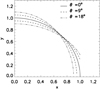 |
Fig. 1. Curves describing intersecting magnetic field lines at different angles from Eq. (1), with ϵ = 0, ϵ = 0.05, and ϵ = 0.1. |
and similarly for y2(x).
Given three points on a x − y plane with coordinates (X1, Y1), (X2, Y2), (X3, Y3), the equation of the circle passing through these points can be written in terms of the following determinant:
where A, B, C, and D are expressions of X1, Y1, X2, Y2, X3, and Y3 and can be derived by expanding the determinant. The centre of the circle is located at (−B/2A,−C/2A), and the radius is given by
 (6)
(6)
Using this analysis, we then found the equation of the circle C1 passing through  , P, and
  and the equation of the circle C2 passing through
  , P, and
  , and we used the radii of these circles as the curvature radius of the magnetic field lines at P.
We applied this analysis, varying l in the range 2−3 ≤ l ≤ 0.2. We find that, in our range of θ and l, the curvature radius ranges between r = 0.99 and r = 1.13. We picked these ranges for θ and l as we focus on small-angle reconnection and relatively local effects. The maximum value of l already corresponds to 20% of the loop radius, and higher values of the angle between the magnetic field lines, θ, are not significantly affected by the curvature radius. In this method, as the magnetic field line equations are not a circle, the parameter l plays a role in the determination of the approximated curvature radius. Figures 2a and b illustrate this configuration for two different values of θ. Moreover, the centres of both circles lie internally with respect to both magnetic field lines. As such a configuration is assumed in equilibrium and the magnetic tension depends on the curvature radius, we associated the curvature radius in this range with an equilibrium configuration.
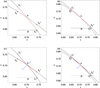 |
Fig. 2. Zoomed-in view of the profiles of intersecting magnetic field lines at θ = 13° (panels a and c) and at θ = 3.7° (b and d). Panels a and b: configuration before the magnetic reconnection, where the connectivity (dashed red arcs) connect ( |


2.1. Post-reconnection magnetic field representation
If we now focus on the effect of a magnetic reconnection event on the magnetic configuration at the point P, we expect the magnetic field lines to become tangent at that point, instead of intersecting. In particular, a new pair of curves is formed. The first one is composed partly by y1 and partly by y2, where we take the two segments of either curve external with respect to the intersection point, P. The other field line is composed by the remaining parts of y1 and y2, such that this is always internal with respect to P. By construction, the curvature radius of these new curves is not analytically defined at P since the derivatives are not continuous at this point, where the analytical expression switches from Eqs. (1) to (2) or vice versa. After the reconnection, the magnetic tension will tend to eliminate the cusp and bring the new field lines into a new configuration.
Using the construction we have previously introduced, the configuration switches from the pair of lines ( , P,
, P,  ), (
), ( , P,
, P,  ) to the pair of lines (
 , P,
, P,  ), (
), ( , P,
, P,  ). When this occurred, in order to estimate the magnetic tension, we computed the curvature radii of the circle Ci, defined by the points (
 , P,
, P,  ), and the circle Ce, defined by the points (
 , P,
, P,  ), which again depend on the value of l.
Figures 2c and 2d illustrate this geometrical construction for the post-magnetic-reconnection configuration. We find that two different scenarios are possible, depending on the values of θ and l. In the first scenario (Fig. 2c), the centres of Ci and Ce are located in two different regions with respect to the magnetic field lines. The centre of Ci is in the interior region, while the centre of Ce is located externally with respect to the magnetic field lines. Because of the curvature, for all values of θ and l, the radius of Ci (ri) is smaller than the radius of Ce (re). The magnetic tension intensity is inversely proportional to the local curvature radius, and, therefore, in this scenario, the inwardly directed magnetic tension is always stronger than the externally directed one. This is represented by the lengths of the blue arrows in Fig. 2c, which are inversely proportional to the curvature radius. The direction of the blue arrows shows the direction of the resulting magnetic tension exerted by both magnetic field lines after reconnection. While this configuration would still allow for a bi-directional jet, the force generated is not symmetric. In the second scenario (Fig. 2d), the centres of both Ci and Ce are located in the interior region, and no external magnetic tension is applied in this case. In other terms, this configuration illustrates the case where both  and
and  lie in the interior part of the loops with respect to P because of the loops’ curvature. This happens when l is large enough for the local curvature around P to become negligible for the circle Ce and the overall curvature of the magnetic field line system becomes dominant.
Figure 3 shows the values of ri and re in logarithm scale when θ = 4° and l is varied. The dashed black lines show the limits of r = 0.99 and r = 1.13, that is, the curvature radius range associated with the equilibrium configuration. We find that, for small values of l, ri is more than an order of magnitude smaller than the equilibrium radius, and only at large values of l does it approach the equilibrium value. In contrast, re is initially very close to ri; however, it rapidly increases to values more than three orders of magnitude larger, where it reaches a cusp maximum. This corresponds to when the three points ( , P,
, P,  ) are in a straight line and we have no magnetic tension. Past this maximum, the convexity of the circle defined by (
 , P,
, P,  ) changes, the exerted magnetic tension flips inward, and re decreases, tending closer to equilibrium values.
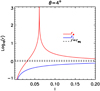 |
Fig. 3. Values of the curvature radii ri (blue line) and re (red line) of the arcs in the post-reconnection field lines as a function of length, l. The dashed black lines represent the minimum and maximum of the curvature radius of the pre-reconnection magnetic field lines. |
Figure 4 shows a colour map of the ratio re/ri to illustrate the θ and l dependence of the ratio between the inward directed and outward directed magnetic tension. We find that where Ce changes convexity, the ratio re/ri reaches a maximum; this happens at larger l the larger θ is. Hence, there is a very well-defined region in the θ − l space that splits the diagram into two parts. On the right-hand side with respect to this region, no outward magnetic tension is allowed and only an inward one can be considered. On the left-hand side, the magnetic tension that generates the inward jet is systematically larger than that generating the outward one. Only at very small values of l are the two forces comparable. However, for any θ, as l increases, the inward magnetic tension becomes increasingly larger.
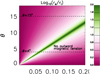 |
Fig. 4. Map of the log of the ratio between re and ri, as a function of length, l, and angle, θ. The dashed lines indicate the cuts where θ = 4° and θ = 15°. |
2.2. Estimate of the time evolution
We now analyse the implication of these regimes for the time evolution of asymmetric jets. In the following analysis of this simplified system, we assume that the magnetic reconnection starts at the smallest spatial scale. Magnetic field lines start reconfiguring by straightening up near the reconnection point, which changes the curvature radius (i.e., the magnetic tension), leading to a new equilibrium. This process therefore evolves, encompassing larger regions, and we define the distance involved in the reconfiguration by the retracting length.
In our analysis the retracting length is represented by the parameter l. This allows us to estimate a time evolution based on the assumption that the retracting length is linearly dependent on time. This can be justified if we assume that the geometry of the field lines (and thus the curvature) does not vary greatly around the reconnection region. Figure 5 can thus be seen as a time evolution of the post-reconnection evolution of the magnetic field lines. When l = 0.01, the global curvature of the magnetic field lines cannot be locally appreciated and the field lines form an x shape, but the global curvature becomes more locally relevant as we move to larger retracting lengths at l = 0.06 and l = 0.11. The panel in the centre (l = 0.06) corresponds to the configuration when the external magnetic field line changes convexity, so we have a bi-directional asymmetric magnetic tension for smaller values of l = 0.06 and a unidirectional internally directed magnetic tension from both field lines for larger values of l = 0.06.
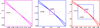 |
Fig. 5. Configuration of the reconnected field lines when θ = 4° at different retracting lengths, l. In each panel we zoom in on a different box around point P; the smaller, interior boxes represent the boxes in the previous panels. The red panel is the largest box, then blue, and the magenta is the smallest. |
Figure 6 shows the logarithm of the ratio between the inward directed magnetic tension and the outward directed one for two different tilt angles, a small-angle case (θ = 4°) and a large-angle case (θ = 15°). In the small-angle case, we find that the ratio quickly reaches values of 103 and that the outward magnetic tension disappears shortly thereafter. For larger tilt angles, however, the increase is slower, and the outward magnetic tension does not disappear in this range of l.
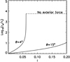 |
Fig. 6. Log of the ratio between re and ri for two different angles, θ. |
In this model we assume the acceleration to be proportional to the force and to be positive away from the reconnection point and negative towards it. Therefore, the force fi = 1/ri, that is, the magnetic tension exerted by the post-reconnection field line ( , P,
, P,  ), is always positive, whereas fe = 1/re, the magnetic tension exerted by the magnetic field line (
 , P,
, P,  ), can be either negative or positive. Additionally, we assume the force fi to be null when the curvature radius is larger than ri = 0.99, the threshold for equilibrium identified in Fig. 3, and the force fe to be null when it falls in the regime where no external magnetic tension is allowed.
We then assumed that the length, l, linearly increases with respect to time, t, and we integrated the equation of motion to find the ratio between the velocities (vi/ve) and the lengths (Si/Se) of the jets as a function of time using a Runge-Kutta scheme. Thus, we have for the velocities
 (7)
(7)
and for the lengths of the jets
 (8)
(8)
We solved the equation of motion between t = 0, when the jets speeds and lengths are 0, and the normalised time, t, which corresponds to our maximum values of l.
Figure 7 shows the ratio between the inward and outward velocities and displacement as a function of time for the small and large tilt angles. We find that for small tilt angles the inward jets accelerate to speeds three times faster than that of the outward jet, whereas the displacement is only up to two times larger. The asymmetry of these jets is consistent at all times and for all the tilt angles, θ, considered. The substantial asymmetry we measured in the tension force is not reflected in this time evolution because it is limited to a small region of the θ − l space. At the same time, we find the asymmetry of the time evolution of the jets to increase significantly for smaller tilt angles, indicating a non-linear evolution.
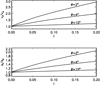 |
Fig. 7. Time evolution of the ratio between the speed of the internal and external jets (top panel) and their displacement (lower panel), for three different values of the angle θ. |
Figure 8 shows the final asymmetry in velocity and displacement in our time evolution for various values of the tilt angle, θ. We find that the asymmetry is small when θ > 10, but it becomes two orders of magnitude larger as we move to the small-angle reconnection regime. Of course, as the tilt angle approaches 0, we approach the limit where no reconnection jet should take place, but this result shows that it is possible to find a regime where reconnection and jets are taking place and the curvature of the loops leads to an asymmetric evolution. Although this is a very simple model, it provides a sense of how the initial misalignment of the curved magnetic field lines significantly affects the asymmetry in the dynamics and lengths of the resulting jets.
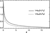 |
Fig. 8. Ratio of the log of the final ratio of the speed (continuous curve) and displacement (dashed curve) between the two jets as a function of the angle θ. |
It should also be noted that the analysis performed here can equally apply to braided field lines, for which, locally, different curvatures exist. The small-angle reconnection regime would be particularly applicable to braided field lines. The directions and speeds of nanojets are therefore likely linked to braiding as well as global loop curvature.
3. MHD modelling
In order to investigate the evolution of reconnection jets from curved magnetic field lines from a different perspective, we devised an MHD model where two magnetic flux systems show interlaced magnetic field lines in a 3D configuration that has some commonalities with what is described in Sect. 2. The aim of these numerical experiments is to verify that the general relations between the asymmetry of the reconnection jets and the geometry of the magnetic configuration we derived in Sect. 2 hold from an MHD perspective as well, even when starting from a mostly symmetric initial configuration. We are not attempting to model solar corona asymmetric reconnection nanojets, as we do not describe the coronal plasma quantities or their evolution.
To develop this model, we used the PLUTO code (Mignone et al. 2012), where the following ideal MHD equations are solved numerically:
 (9)
(9)
 (10)
(10)
 (11)
(11)
 (12)
(12)
where t is the time, v is the velocity, pt is the total pressure (i.e., the sum of gas pressure, p, and magnetic pressure, pm), B is the magnetic field,  is the current density, c is the speed of light, and I is the identity tensor. The total energy density, E, is given by
 (13)
(13)
where γ = 5/3 denotes the ratio of specific heats.
3.1. Initial conditions and numerical setup
In our model, the initial configuration consists of two shifted arcade systems defined in a Cartesian reference frame (x, y, z) that extends from x = −50 Mm to x = 50 Mm in the x direction, from y = 2.5 Mm to y = 52.50 Mm in the y direction, and from z = −0.78125 Mm to y = +0.78125 Mm in the z direction. The arcade systems develop on the x − y plane and are defined by the magnetic field components
 (14)
(14)
 (15)
(15)
where ±xc is a model parameter that is taken with its positive value for z ≥ 0 and its negative value for z < 0. In this way, two identical configurations shifted by 2xc along the x axis coexist in the domain, and one switches into the other across the plane z = 0. Moreover, the angle between the magnetic field vector defined in z < 0 and that defined in z > 0 are uniform. The general direction of the magnetic field lines does not change, so the two flux systems show only a small misalignment with respect to each other.
In this model we adopt a configuration where the two flux systems are locally magnetically connected, such that the magnetic reconnection has already occurred around the point (xJ = 0,yJ = 25,0). In order to describe this post-reconnection configuration, we added a z component of the magnetic field,
 (16)
(16)
where Bz0 = 1.1 G, L⊥ = 0.25 Mm, and L∥ is a parameter that controls the extension in the x direction of the region in which this connecting component is present.
The x and y components of the magnetic field are force-free by construction; therefore, adding this z component of the magnetic field generates unbalanced magnetic pressure gradient and magnetic tension. In particular, the inward magnetic tension (towards the origin of the axes) is slightly (2%) more intense than the outward magnetic tension (away from the origin). Such a construction is clearly different from the analytical one, where we estimated an orders-of-magnitude difference between the inward and outward magnetic tension. With this numerical experiment, we aim at showing that the MHD evolution that follows the triggering of the jets also adds asymmetry to the jets’ evolution.
The density in our initial conditions is defined as
![Mathematical equation: $$ \begin{aligned} \rho =2\rho _{D}+\frac{\left(0.5\rho _0-\rho _D\right)}{2} \left[\left(1+\tanh {\left({ y}-5\right)}\right)+ \left(1+\tanh {\left(50-{ y}\right)}\right)\right] ,\end{aligned} $$](/articles/aa/full_html/2021/12/aa41030-21/aa41030-21-eq53.gif) (17)
(17)
where ρ0 = 4.2 g cm−3 and ρD = 103ρ0. With such a density distribution we have a density value of ρD in two regions of 5 Mm in width near the two y boundaries and ρ0 elsewhere. The purpose of these high density regions is to slow the propagation of perturbations from the y boundaries so as to avoid artificial boundary effects. Finally, the thermal pressure distribution is constructed to have a uniform total pressure, pT = p + B2/8π = 0.42 erg cm−3, corresponding to a value of β = p/(B2/8π) = 0.47 around the location (0,yJ). In this configuration, only the magnetic tension introduced by Bz remains as an unbalanced force that can drive the dynamics of the numerical experiment. Finally, the temperature is derived from the pressure, and the density from the ideal equation of state.
Figure 9 shows a density map on the z = 0 plane, where we also plot magnetic field lines for z > 0 (magenta lines) and z < 0 (green lines) when we set xc = 0.5 Mm. The central blue box is the domain around the location (xJ,yJ), where we focus our investigation. We set up this simulation in a grid of 4096 × 2048 × 64 cubic cells with a spatial resolution of Δx = Δy = Δz = 0.024 Mm. We used outflow boundary conditions at the y boundaries and periodic boundary conditions at the x and z boundaries. The outflow y boundaries are not force-free, and thus the presence of the high density regions is key to maintaining the centre of the domain unperturbed for a long enough time to study the evolution around (xJ,yJ). Moreover, we do not use a magnetic field divergence cleaning technique, as the magnetic field evolution is computed using the constrained transport approach (Balsara & Spicer 1999).
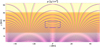 |
Fig. 9. Map of density in the z = 0 plane in the initial condition of the MHD simulations. The maximum in this map is at ρ = 6 × 10⁻¹⁴ g cm−3. Green lines show the magnetic field lines for z < 0 and magenta lines for z > 0 when we set xc = 0.5 Mm. |
3.2. Numerical simulations
Figure 10 shows some of the different initial configurations we considered. In the top row panels, we show maps of Bz with some magnetic field lines overplotted. We take the left-hand side column simulation as the reference one. The central column simulation differs from the reference one in the angle between the magnetic field lines of the two flux systems (i.e., larger values of the parameter xc) and the right-hand side column simulation in the wider region where a Bz is present (i.e., larger values of the parameter L⊥). In the bottom panels we zoom in to the region around (xJ, yJ), and we plot some magnetic field lines projected onto the x − y and x − z planes, which are coloured black and orange if they cross the z = 0 plane (i.e., reconnected magnetic field lines) and are coloured magenta and green if they remain in the same arcade system. It should be noted that, in this configuration, Bz bridges the two arcade systems across the current sheet over a length of ∼0.1 Mm, which corresponds to four cells. In this set of simulations, we vary the parameters xc and L∥. By changing the parameter xc, the two arcade systems become more shifted in x and the angle between the field lines from different arcades, θ, increases. We considered three values of xc so as to have θ = 3.6°, θ = 7.2°, and θ = 14.4°. As for the extension of the Bz distribution, we ran simulations with L∥ = 0.5 Mm, L∥ = 1.0 Mm, and L∥ = 2.0 Mm. The simulation with θ = 3.6° and L∥ = 0.5 Mm was used as reference, and any other simulation varies only one of the two parameters, leading to a total of five simulations.
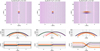 |
Fig. 10. Upper row: maps of Bz in the initial conditions of our simulations with superimposed magnetic field lines (green for z < 0 and magenta for z > 0), where we set xc = 0.5 Mm and L∥ = 0.5 Mm (left-hand column), xc = 2.0 Mm and L∥ = 0.5 Mm (central column), and xc = 0.5 Mm and L∥ = 2.0 Mm (right-hand column) on the plane z = 0. Two lower rows: some representative magnetic field lines projected onto the x − y plane and x − z planes. Magnetic field lines are coloured black and orange if they cross the z = 0 plane, and magenta and green if they do not. |
3.3. Evolution in the reference simulation
Our reference simulation has θ = 3.6° and L∥ = 0.5 Mm. Its evolution is qualitatively similar to the other simulations, and we thus illustrate only this one in greater detail. Figure 11a shows the radial component of the out-of-equilibrium magnetic tension in the initial condition. To measure this quantity, we compared this magnetic configuration with an analogous one where we used Bz0 = 0. We find that the magnetic tension pushes the plasma outwards from the reconnection region, being positive above yJ and negative below. The intensity of the magnetic tension above (below) yJ pushing the plasma upwards (downwards) is roughly the same. This is an important difference in the construction of this MHD model with respect to the analytical construction sketched in Fig. 2, where the inwardly directed magnetic tension is larger than the outwardly directed one. However, this difference holds only for the initial condition; as soon as the system starts evolving, the inwardly directed magnetic tension becomes slightly, but consistently, larger than the outwardly directed one.
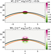 |
Fig. 11. (a) Map of the difference in the radial component of the magnetic tension between our simulation with xc = 0.5 Mm and L∥ = 0.5 Mm and the analogous magnetic tension in a configuration where we set Bz0 = 0 on the plane z = 0. (b) Radial component of the gradient of the total pressure at t = 10 s in the same simulation as (a). In both panels some representative field lines are superimposed. |
As soon as the plasma starts moving, a total pressure gradient develops. Figure 11b shows the radial component of the total pressure gradient at t = 10 s. The total pressure distribution presents a complex structure, generally contrasting the magnetic tension, and it thus acts to slow down the plasma flows since it is half as intense as the magnetic tension.
Such forces lead to a bi-directional jet evolution. One jet propagates outwards with respect to the curvature of the magnetic field (above yJ), while the other jet propagates inwards (below yJ). The evolution of the simulation can be summarised in the three key stages represented in Fig. 12, where we plot the projection of the radial velocity onto the direction perpendicular to the magnetic field, VJ, at different times. The dashed contours in Fig. 12 limit the region above and below the origin of the jets where VJ is, respectively, positive or negative, with a magnitude above 5 m s−1. This is the component of the velocity that moves outwards from (0,yC) and is caused by the magnetic tension. In the very early stage of the evolution, the quantity VJ captures a magnetoacoustic perturbation moving away from the reconnection point and which is not relevant for our study. This perturbation is still visible at t = 10 s as two semicircles. However, at the same time, within 0.5 Mm of the (0,yC) point, we find a higher velocity where the plasma moves outwards, accelerated by magnetic tension. At a later time, VJ (and its contour) properly describes the jets’ evolution since their speeds then drop as they start interacting with the background medium. Such velocities, modest in comparison to what is normally observed in the solar corona, can be explained by the model parameters that have been chosen for these numerical experiments. In particular, the high plasma density, the plasma (β) being higher than in solar active regions, and the low magnetic field intensity contribute to forming jets that have velocities lower than the typical velocities observed in the solar corona. It should be noted, however, that during the evolution we find a decrease in magnetic energy in the proximity of the reconnection point that is fully converted into kinetic (jets) and thermal (compression) energy. The magnetic energy conversion is approximately the amount of magnetic energy initially stored in the Bz component of the magnetic field. These energetic considerations indicate that the energy of the jets depends on how much free magnetic energy is available in the initial condition.
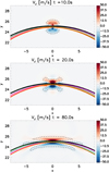 |
Fig. 12. Maps of the velocity of the jets, VJ, defined as the projection of the radial velocity onto the direction perpendicular to the magnetic field at three different times in the simulation with xc = 0.5 Mm and L∥ = 0.5 Mm on the z = 0 plane. In all panels some representative field lines are superimposed. Dashed black contours show the region where the jet speed is above 5 m s−1; it is positive for the region above yJ and negative for the region below yJ. |
In the last phase, the jets continue expanding, mostly in the y direction, for some time, and at t = 20 s we find two larger regions with positive and negative velocities. The jets’ deceleration phase is longer than the acceleration phase but is still effective within the timescale of our simulation since the jets’ speed drops to half of their maximum speed in 75 s. In this last phase, represented by t = 80 s, we find that the jets slow and, as a result, the motion also spreads along the x direction. During this evolution the magnetic field lines reconfigure in such a way that the intensity of the magnetic tension decreases.
In order to measure the asymmetry between these jets, we considered the kinetic energy associated with the jet velocity (i.e.,  ), and we computed the integral across the horizontal cut at various y coordinates in the region within the dashed contours in Fig. 12. Figure 13a shows a map of the quantity EJ as a function of time and y coordinates. We find that the kinetic energy concentrates in the regions just below and above yJ (dashed line in Fig. 13), and it decreases during the MHD simulation because of the jet deceleration. The initial structures (t < 15 s) propagating symmetrically from yJ are due to the fast magnetoacoustic perturbations and are already far enough from the origin of the jets at t = 15 s. After t = 15 s, instead, the energy directly associated with the jets becomes predominant in the map as two bands that grow and then remain approximately at the same y location from t = 50 s. In particular, the lower region consistently shows higher kinetic energy values.
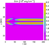 |
Fig. 13. Time-space map of the distribution of the integral of EJ across the x direction in the simulation with xc = 0.5 Mm and L∥ = 0.5 Mm on the z = 0 plane. |
Figure 14 shows the evolution of the quantity EJ integrated in the region above the yC (red lines) and below it (blue lines) for three different simulations. We include for reference the other two simulations, where we change either the angle, θ, or the extent of the Bz distribution, L∥. For all the simulations, the evolution always remains asymmetric, meaning the inward propagating jets always carry more energy than the outward counterparts.
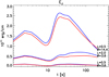 |
Fig. 14. Time evolution of the integral of EJ in the region above (red lines) and below (blue line) yJ for three different simulations. The parameters are listed in the plot. |
During the very first stage of the evolution, when the magnetoacoustic perturbations are still present, the evolution is still symmetric, but it becomes increasingly more asymmetric as the jets accelerate (t < 20 s). Additionally, we find that the energy of the jets is different for different configurations as it increases when we either increase L∥ or θ. In particular, the simulation with a higher tilt angle between the two arcade systems leads to the most energetic jets. Naturally, these stronger jets incur the most effective damping as they interact with the background medium. Moreover, as the magnetic field intensity is higher below the reconnection point, the inwardly directed jets are more effectively decelerated. This effect becomes more important the larger the displacement of the jets is. For this reason, the inward jet of the simulation with θ = 14.4° eventually becomes slower than the outward jet (t ∼ 150 s).
It should be noted that the initial condition of this MHD model shows a nearly symmetric configuration of the initial magnetic tension forces that generate the jets. However, the asymmetry in the jets still develops and increases in times as they accelerate. This corroborates that the curvature of the magnetic field affects the symmetry of the jets not only when they are generated, but also during their acceleration phase.
3.4. Dependence on model parameters
In order to inspect the model we describe in Sect. 2, we looked into the dependence on the angle between the reconnecting field lines, θ (the tilt angle), and the dependence on the width of the Bz distribution (i.e., L∥). We therefore considered the simulations where we increase either parameters. In order to compare how the asymmetry of the jets develops, for all these simulations we measured the ratio of the integral of EJ below and above the reconnection point as a function of time (see Fig. 14).
Figure 15a shows how this ratio evolves for the simulations where we vary the θ parameter. In all cases, the evolution shows a similar pattern, in which the ratio initially increases, reaches a maximum, and finally decreases during the jets’ deceleration phase. In this setup, the peak of asymmetry is dependent on the angle, as predicted in Sect. 2. Indeed, the simulations with a higher angle consistently show a lower degree of asymmetry at all times.
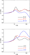 |
Fig. 15. (a) Time evolution of the asymmetry of the jets (ratio between the integral of EJ below and above yJ) for the three simulations, differing in terms of the angle θ. (b) Time evolution of the asymmetry of the jets for the three simulations, differing in terms of the width of the initial Bz distribution, L∥. |
Figure 15b shows the evolution of the asymmetry for the simulations where we vary the width of the Bz distribution. Also in this case, the evolution shows a similar pattern of an initial increase followed by a maximum and, finally, a decrease. However, this happens on different timescales, where the simulation with L∥ = 2 is the slowest in reaching a maximum. The comparison now with our results in Sect. 2 is less evident since the width of the Bz distribution is not obviously associated with the retracting length. However, for both parameters, the larger their value is, the larger the portion of the curved magnetic field lines involved is and the more the global curvature of the loop becomes important. At the same time, in Sect. 2 we assumed that the retracting length varies in time as the reconnection occurs locally but that the reconfiguration then expands from there. Such behaviour is not reproduced in these MHD simulations, where the parameter L∥ only affects the initial condition.
However, none of these simulations reproduces the regime described in Sect. 2, where there is no outward directed magnetic tension force. This is because the reconnected magnetic field is inherent to the initial condition, and we thus always have an outward directed magnetic tension. Another significant difference between this approach and the one in Sect. 2 is that in these simulations the width of the region affected by the reconnection is determined from the beginning and does not grow in time as in Sect. 2.2. Because of this, the asymmetric growth of the magnetic tension force described in Sect. 2.2 cannot be reproduced by the MHD simulations, where, in contrast, the asymmetry in the magnetic tension force is maximum at the initial condition and then slightly decreases in time.
4. Discussion and conclusions
In this work we have investigated the asymmetric nature of reconnection jets from curved magnetic field lines. The nanojets in the solar corona (Antolin et al. 2021) are an example of these phenomena. We focused on some probable explanations for such asymmetry and addressed this problem from two points of view: first, using a simple geometrical model to explain why we expect asymmetric jets; and second, using MHD simulations to analyse the evolution of these phenomena after the reconnection has taken place.
The observations show that nanojets show a preferential direction of propagation inward with respect to the curvature of the hosting coronal loop. Our investigation suggests that such dynamics can be explained by the larger inward magnetic tension forces generated when two curved magnetic field lines reconnect.
Using our simple geometrical model, we have shown that the global curvature of the loop contributes to the local magnetic field line curvature that is formed as a consequence of the magnetic reconnection. Therefore, the curved magnetic field environment breaks the symmetry for the otherwise perfectly bi-directional nanojets and causes the inwardly directed flow to exceed the outwardly directed one.
These asymmetric effects become less relevant as the misalignment angle between the reconnecting magnetic field line increases since this leads to higher local curvatures at the reconnection point that exceed the global curvature of the coronal loop. This effect, however, can be compensated for when the retracting length of the magnetic field lines involves a larger region since, in this case once again, the global curvature dominates over the local one.
In our geometrical model we also find two different possible regimes, one where the nanojets are generated by asymmetric tension forces and a second where the outward tension simply cannot be generated. Our analytical model is mostly based on the local curvature of the field lines at both sides of the reconnection point, which here is controlled by the global curvature of the field lines. Hence, our analysis is not only valid for loop curvatures but can easily be generalised to any kind of factor that leads to a local curvature, such as loop braiding. Along this line of thought, if the local curvature introduced by braiding is more important than that set by the loop curvature, it is likely that nanojets are not exclusively inwardly directed but instead may move in any direction while still being unidirectional.
When we approach the problem from an MHD perspective, we find consistent results but also interesting differences. In order to study the jets in MHD, we devised a two-arcade system in which one arcade is shifted to near the other and the two are separated by a current sheet. A connecting magnetic field is enforced to model the post-reconnection magnetic configuration, and the magnetic tension generated in this way pushes the plasma away, leading to two jets, one inwardly and one outwardly directed. In the MHD framework, we recover some of the analytical results, such as that the jets become more symmetric as the misalignment angle between the magnetic field lines increases and that they become more asymmetric with a wider region across which magnetic field lines are connected. Crucially, the MHD simulations confirm that the inward jets are consistently more energetic than the outward ones.
On the other hand, MHD simulations cannot reproduce the regime where no outward flow exists, and this is because the imposed magnetic field inherently causes a bi-directional jet. Additionally, the jets in the MHD simulations show a significantly smaller asymmetry as the inward jets are not orders of magnitude more energetic, unlike what is prescribed by the analytical model. This is probably because the MHD model starts with a symmetric force that triggers the jets and does not comprehensively describe the time evolution of the magnetic reconnection.
In the follow-up of this work, we aim at running MHD simulations with an explicit resistivity term that allows the magnetic reconnection and the evolution of the jets to be simultaneously studied in a full MHD framework. We expect such numerical experiments to develop more complex flows since the magnetic field diffusion and the temporary cancellation of the magnetic field before the reconnection will lead to plasma flows along the magnetic field lines because of the magnetic pressure gradient. Additionally, the magnetic diffusion inevitably leads to ohmic heating, which will trigger further plasma flows.
In this work we find that when the reconnection angle is small enough and the region involved in the reconnection is large enough, nanojets can be substantially asymmetric. This finding reconciles our model with the observational evidence found in Antolin et al. (2021). However, in Antolin et al. (2021) the large majority of the observed jets were unidirectional, and such a high degree of asymmetry is not matched in the MHD simulations presented here.
In conclusion, this modelling work establishes as proof of concept that the curvature of magnetic structures affects the symmetry of local reconnection jets, but a more complete MHD model needs to be developed to fully explain this mechanism and bridge the gap with observations. Also, additional observations of nanojets are needed to consolidate this description. In particular, high resolution observations and accurate reconstructions of the coronal magnetic field are necessary to ultimately validate this approach.
Acknowledgments
P.A. acknowledges funding from STFC Ernest Rutherford Fellowship (No. ST/R004285/2). This work used the DiRAC@Durham facility managed by the Institute for Computational Cosmology on behalf of the STFC DiRAC HPC Facility (www.dirac.ac.uk). The equipment was funded by BEIS capital funding via STFC capital grants ST/P002293/1, ST/R002371/1 and ST/S002502/1, Durham University and STFC operations grant ST/R000832/1. DiRAC is part of the National e-Infrastructure. PLUTO was developed at the Turin Astronomical Observatory in collaboration with the Department of Physics of the Turin University. A.P. acknowledges financial contribution from the agreement ASI-INAF n.2018-16-HH.0.
References
- Antolin, P., Shibata, K., Kudoh, T., Shiota, D., & Brooks, D. 2008, ApJ, 688, 669 [NASA ADS] [CrossRef] [Google Scholar]
- Antolin, P., Pagano, P., Testa, P., Petralia, A., & Reale, F. 2021, Nat. Astron., 5, 54 [NASA ADS] [CrossRef] [Google Scholar]
- Archontis, V., & Hood, A. W. 2013, ApJ, 769, L21 [Google Scholar]
- Axford, W. I. 1984, Washington DC American Geophys. Union Geophys. Monogr. Ser., 30, 1 [NASA ADS] [Google Scholar]
- Balsara, D. S., & Spicer, D. S. 1999, J. Comput. Phys., 149, 270 [NASA ADS] [CrossRef] [Google Scholar]
- Cassak, P. A., & Shay, M. A. 2007, Phys. Plasmas, 14 [Google Scholar]
- Chitta, L. P., Peter, H., Young, P. R., & Huang, Y. M. 2017, A&A, 605, A49 [NASA ADS] [CrossRef] [EDP Sciences] [Google Scholar]
- Hudson, H. S. 1991, Sol. Phys., 133, 357 [Google Scholar]
- Ishikawa, S., Glesener, L., Krucker, S., et al. 2017, Nat. Astron., 1, 771 [NASA ADS] [CrossRef] [Google Scholar]
- Klimchuk, J. A. 2015, Philos. Trans. R. Soc. London Ser. A, 373, 20140256 [NASA ADS] [Google Scholar]
- Marshall, A. T., Burch, J. L., Reiff, P. H., et al. 2020, J. Geophys. Res. (Space Phys.), 125 [Google Scholar]
- Martínez-Sykora, J., De Pontieu, B., Hansteen, V. H., et al. 2017, Science, 356, 1269 [Google Scholar]
- Mignone, A., Zanni, C., Tzeferacos, P., et al. 2012, ApJS, 198, 7 [Google Scholar]
- Moriyasu, S., Kudoh, T., Yokoyama, T., & Shibata, K. 2004, ApJ, 601, L107 [NASA ADS] [CrossRef] [Google Scholar]
- Murphy, N. A., & Lukin, V. S. 2015, ApJ, 805, 134 [Google Scholar]
- Nelson, C. J., Shelyag, S., Mathioudakis, M., et al. 2013, ApJ, 779, 125 [Google Scholar]
- Parker, E. N. 1988, ApJ, 330, 474 [Google Scholar]
- Reale, F. 2014, Liv. Rev. Sol. Phys., 11, 4 [Google Scholar]
- Shibata, K. 2005, AIP Conf. Ser., 784, 153 [NASA ADS] [CrossRef] [Google Scholar]
- Shibata, K., Nakamura, T., Matsumoto, T., et al. 2007, Science, 318, 1591 [Google Scholar]
- Solanki, R., Srivastava, A. K., & Dwivedi, B. N. 2020, Sol. Phys., 295, 27 [NASA ADS] [CrossRef] [Google Scholar]
- Takasao, S., Asai, A., Isobe, H., & Shibata, K. 2012, ApJ, 745, L6 [Google Scholar]
- Testa, P., De Pontieu, B., Martínez-Sykora, J., et al. 2013, ApJ, 770, L1 [NASA ADS] [CrossRef] [Google Scholar]
- Testa, P., De Pontieu, B., Allred, J., et al. 2014, Science, 346, 1255724 [Google Scholar]
- Tian, H., Kleint, L., Peter, H., et al. 2014, ApJ, 790, L29 [Google Scholar]
- van Ballegooijen, A. A., Asgari-Targhi, M., Cranmer, S. R., & DeLuca, E. E. 2011, ApJ, 736, 3 [Google Scholar]
All Figures
|
Fig. 1. Curves describing intersecting magnetic field lines at different angles from Eq. (1), with ϵ = 0, ϵ = 0.05, and ϵ = 0.1. |
| In the text | |
|
Fig. 2. Zoomed-in view of the profiles of intersecting magnetic field lines at θ = 13° (panels a and c) and at θ = 3.7° (b and d). Panels a and b: configuration before the magnetic reconnection, where the connectivity (dashed red arcs) connect ( |
| In the text | |
|
Fig. 3. Values of the curvature radii ri (blue line) and re (red line) of the arcs in the post-reconnection field lines as a function of length, l. The dashed black lines represent the minimum and maximum of the curvature radius of the pre-reconnection magnetic field lines. |
| In the text | |
|
Fig. 4. Map of the log of the ratio between re and ri, as a function of length, l, and angle, θ. The dashed lines indicate the cuts where θ = 4° and θ = 15°. |
| In the text | |
|
Fig. 5. Configuration of the reconnected field lines when θ = 4° at different retracting lengths, l. In each panel we zoom in on a different box around point P; the smaller, interior boxes represent the boxes in the previous panels. The red panel is the largest box, then blue, and the magenta is the smallest. |
| In the text | |
|
Fig. 6. Log of the ratio between re and ri for two different angles, θ. |
| In the text | |
|
Fig. 7. Time evolution of the ratio between the speed of the internal and external jets (top panel) and their displacement (lower panel), for three different values of the angle θ. |
| In the text | |
|
Fig. 8. Ratio of the log of the final ratio of the speed (continuous curve) and displacement (dashed curve) between the two jets as a function of the angle θ. |
| In the text | |
|
Fig. 9. Map of density in the z = 0 plane in the initial condition of the MHD simulations. The maximum in this map is at ρ = 6 × 10⁻¹⁴ g cm−3. Green lines show the magnetic field lines for z < 0 and magenta lines for z > 0 when we set xc = 0.5 Mm. |
| In the text | |
|
Fig. 10. Upper row: maps of Bz in the initial conditions of our simulations with superimposed magnetic field lines (green for z < 0 and magenta for z > 0), where we set xc = 0.5 Mm and L∥ = 0.5 Mm (left-hand column), xc = 2.0 Mm and L∥ = 0.5 Mm (central column), and xc = 0.5 Mm and L∥ = 2.0 Mm (right-hand column) on the plane z = 0. Two lower rows: some representative magnetic field lines projected onto the x − y plane and x − z planes. Magnetic field lines are coloured black and orange if they cross the z = 0 plane, and magenta and green if they do not. |
| In the text | |
|
Fig. 11. (a) Map of the difference in the radial component of the magnetic tension between our simulation with xc = 0.5 Mm and L∥ = 0.5 Mm and the analogous magnetic tension in a configuration where we set Bz0 = 0 on the plane z = 0. (b) Radial component of the gradient of the total pressure at t = 10 s in the same simulation as (a). In both panels some representative field lines are superimposed. |
| In the text | |
|
Fig. 12. Maps of the velocity of the jets, VJ, defined as the projection of the radial velocity onto the direction perpendicular to the magnetic field at three different times in the simulation with xc = 0.5 Mm and L∥ = 0.5 Mm on the z = 0 plane. In all panels some representative field lines are superimposed. Dashed black contours show the region where the jet speed is above 5 m s−1; it is positive for the region above yJ and negative for the region below yJ. |
| In the text | |
|
Fig. 13. Time-space map of the distribution of the integral of EJ across the x direction in the simulation with xc = 0.5 Mm and L∥ = 0.5 Mm on the z = 0 plane. |
| In the text | |
|
Fig. 14. Time evolution of the integral of EJ in the region above (red lines) and below (blue line) yJ for three different simulations. The parameters are listed in the plot. |
| In the text | |
|
Fig. 15. (a) Time evolution of the asymmetry of the jets (ratio between the integral of EJ below and above yJ) for the three simulations, differing in terms of the angle θ. (b) Time evolution of the asymmetry of the jets for the three simulations, differing in terms of the width of the initial Bz distribution, L∥. |
| In the text | |
Current usage metrics show cumulative count of Article Views (full-text article views including HTML views, PDF and ePub downloads, according to the available data) and Abstracts Views on Vision4Press platform.
Data correspond to usage on the plateform after 2015. The current usage metrics is available 48-96 hours after online publication and is updated daily on week days.
Initial download of the metrics may take a while.