| Issue |
A&A
Volume 656, December 2021
|
|
|---|---|---|
| Article Number | A123 | |
| Number of page(s) | 13 | |
| Section | Galactic structure, stellar clusters and populations | |
| DOI | https://doi.org/10.1051/0004-6361/202040189 | |
| Published online | 10 December 2021 | |
A cusp-core-like challenge for modified Newtonian dynamics
CP3-Origins, University of Southern Denmark, Campusvej 55, 5230 Odense M, Denmark
e-mail: This email address is being protected from spambots. You need JavaScript enabled to view it.
, This email address is being protected from spambots. You need JavaScript enabled to view it.
, This email address is being protected from spambots. You need JavaScript enabled to view it.
Received:
21
December
2020
Accepted:
4
September
2021
Abstract
We show that modified Newtonian dynamics (MOND) predicts distinct galactic acceleration curve geometries – in the space of total observed centripetal accelerations, gtot, versus the inferred Newtonian acceleration from baryonic matter, gN, which we refer to as g2 space – and corresponding rotation speed curves. MOND modified gravity predicts cored geometries for isolated galaxies, while MOND modified inertia yields neutral geometries (i.e. neither cuspy nor cored), based on a cusp-core classification of galaxy rotation curve geometry in g2 space, rather than on inferred dark matter (DM) density profiles. The classification can be applied both to DM and modified gravity models as well as data and implies a ‘cusp-core’ challenge for MOND from observations (e.g., of cuspy galaxies), which is different from the so-called cusp-core problem of DM. We illustrate this challenge with a number of cuspy and cored galaxies from the SPARC rotation curve database that deviate significantly from the MOND modified gravity and MOND modified inertia predictions.
Key words: dark matter / methods: data analysis / Galaxy: structure
© ESO 2021
1. Introduction
The missing mass problem in astrophysical systems, from galaxies and galaxy clusters to the cosmic microwave background, is well established. Gravitational potentials are observed to be deeper than predicted from the visible matter distributions in Newtonian gravity. Early observations of this phenomenon include the velocity dispersion of galaxies in clusters (Zwicky 1933) and galactic rotation curves (Rubin & Ford 1970; Rubin et al. 1980; Bosma 1981). Both particle dark matter (DM; Lee & Weinberg 1977; Steigman & Turner 1985) and modified Newtonian dynamics (MOND; Milgrom 1983) were proposed as explanations of these observations. In MOND, the acceleration of test particles is modified, with respect to the Newtonian prediction, below a characteristic acceleration scale g0 ∼ 10−10 m s−2 to yield asymptotically constant speeds in rotation curves at large radii and low accelerations (Sanders & McGaugh 2002; Gentile et al. 2011; McGaugh et al. 2016; Lelli et al. 2017; Li et al. 2018), as observed. MOND also provides a correlation of this asymptotic speed with the total baryonic mass in the galaxy, that is, the baryonic Tully-Fisher relation (Tully & Fisher 1977; McGaugh et al. 2000). However, it has been argued that MOND cannot account for the entire missing mass observed in galaxy clusters (Sanders 2003), and today the more recent observations of merging clusters (Clowe et al. 2006) and the measurements of the cosmic microwave background (Skordis et al. 2006; Dodelson & Liguori 2006; Dodelson 2011) are considered by many as a challenge for MOND. A review of MOND and observations are available in Famaey & McGaugh (2012). Despite these known challenges, it is of obvious interest to investigate in detail the predictions of MOND for rotation curves beyond the asymptotic velocities at large radii.
Recently, the sample of galaxies in the SPARC database was compared to a MOND modified inertia (MI) model, and it was found that the fit residuals were Gaussian and of the expected size (McGaugh et al. 2016; Lelli et al. 2017; Li et al. 2018). However, in Frandsen & Petersen (2018) it was shown that data at small radii deviate significantly from the MOND MI fit. Since the sample of data at small radii is only a few hundred points, compared to the few thousand points at large radii, the discrepancy is only apparent in the residuals if these data are treated separately (see Fig. 5) or if galaxies are considered individually (Petersen & Frandsen 2020, see also Fig. 4). Investigating data points at small radii separately is well motivated as this is where the predictions of different models of the missing mass problem deviate significantly. In particular, MOND modified gravity (MG) and MOND MI models only deviate in their predictions in a definite manner at small radii, as we show here.
Early simulations of structure formation with cold collisionless DM particles and no baryons found universal cuspy Navarro-Frenk-White-like DM density profiles in halos ranging from dwarf galaxies to galaxy clusters (Navarro et al. 1996). This profile fits rotation curve data at large radii in galaxies and clusters, but not in all cases at small radii. The inferred DM densities from some observed clusters and gas-rich halo-dominated dwarf spirals is less steep (i.e., more cored) than the NFW profile in the inner regions (Flores & Primack 1994). This has become known as the cusp-core problem for DM. More recent DM-only simulations have found some systematic departures from the NFW profile and some diversity in the resulting rotation curves (Navarro et al. 2010). However, these DM-only simulations still show little variation in rotation curve profiles with the same asymptotic maximal rotational velocity (Oman et al. 2015), while observed rotation curves of dwarf galaxies do show such a variation. This has been termed the diversity problem. Whether the cusp-core problem or the diversity problem is a problem of DM, or rather of simulations with limited resolution and without the inclusion of baryons, remains a topic of debate since simulations that include baryonic feedback do find cored profiles (Read & Gilmore 2005; Teyssier et al. 2013; Di Cintio et al. 2014).
In this paper we identify a different related cusp-core challenge pertaining to MOND that is essentially the opposite of that for DM. To do so, we first provide a definition and classification of cuspy, neutral, and cored galaxies. The definition is based on acceleration curve geometry in g2 space following Frandsen & Petersen (2018) (i.e., the space of total centripetal accelerations, gobs, versus the Newtonian centripetal acceleration from baryonic matter, gbar) rather than on inferred DM density profiles. This classification is directly applicable to both MOND and DM models. Throughout this paper we refer to this new definition of cuspy and cored galaxies unless otherwise stated.
We show that MOND MG models, in the Bekenstein-Milgrom formulation, lead to cored acceleration curve geometries in g2 space and corresponding rotation speed curves – a consequence of the so-called solenoidal acceleration field in these models. We first illustrate this using analytical approximations (Brada & Milgrom 1994) and by investigating the curl of the solenoidal field, before we explicitly solve the MOND modified Poisson equation using the N-Mody code (Ciotti et al. 2006). In contrast, MOND MI curves provide a definition of ‘neutral’ curves, neither cuspy nor cored, as a benchmark.
A way to test MOND MG is therefore to look for cuspy galaxies according to our definition as well as cored galaxies that deviate from the specific cored geometries predicted by MOND MG models. We identify such galaxies in the SPARC database, extending our previous analyses of MOND MI models (Petersen & Frandsen 2020; Frandsen & Petersen 2018).
The paper is organized as follows. In Sect. 2 we present our definition and classification of cuspy, neutral, and cored galaxies based on acceleration curve geometry in g2 space. In Sect. 3 we show that MOND MG yields cored rotation curve geometries, which tend to neutral geometries for spherical mass distributions. We show this using general properties of the MOND solenoidal field, analytic approximations (Brada & Milgrom 1994), and full numerical solutions using the N-Mody code Ciotti et al. (2006). On the other hand, MOND MI universally leads to neutral rotation curve geometries, independent of the matter distribution. We note that Banik et al. (2018) also compares aspects of the analytical approximations in Brada & Milgrom (1994) to numerical simulations of the quasi-linear version of MOND MG, QUMOND. In Sect. 4 we identify cored and cuspy acceleration curve examples from the SPARC database of galaxies and compare them to the model predictions before giving our summary.
2. Classification of cuspy, cored, and neutral geometries in g2 space
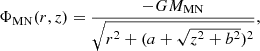
We begin by reviewing the geometric characteristics of galactic centripetal acceleration curves, which we refer to as g2-space curves – the space of total predicted1 centripetal accelerations, gtot, versus the Newtonian acceleration from baryons, gN – following Frandsen & Petersen (2018). Examples of MOND MG and MOND MI curves in g2 space are shown in the top panel of Fig. 1.
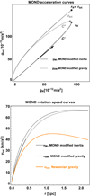 |
Fig. 1. Top panel: centripetal acceleration curves in g2 space with the quantities rtot, rN, and 𝒞±, used for classification in Table 1, shown. The solid grey line shows a MOND MI curve with the radius of maximum baryonic acceleration and maximum total acceleration rN = rtot indicated. Also, the curve segments 𝒞+ and 𝒞− coincide, so the curve area is 𝒜(𝒞) = 0. The dotted grey and dotted black curves show the 𝒞± curve segments of a MOND MG curve, using the Brada-Milgrom approximation in Eq. (9), with rtot > rN and 𝒜(𝒞) > 0. For both, the baryonic matter is an infinitely thin exponential disc, Σ(r) = Σ0e−r/rd. The arrow indicates the direction of increasing radius along the curve. Bottom panel: corresponding rotation curves. |
Geometric characteristics of cuspy, neutral, and cored geometries of rotation acceleration curves.
We first defined the radii rtot and rN as the locations at which the centripetal accelerations, gtot and gN, are maximum:
 (1)
(1)
These radii are indicated in the top panel of Fig. 1 and coincide for MOND MI, while rtot > rN for MOND MG. From these radii we defined the acceleration ratios,
 (2)
(2)
relevant for reducing systematic uncertainties when we study SPARC data (Frandsen & Petersen 2018).
We classified galaxies as cuspy if rtot < rN, neutral if rtot = rN, and cored if rtot > rN. More generally, we are interested in the relative location of the entire curve segment C+ at large radii and that at small radii C− defined with respect to rN:
 (3)
(3)
Galaxies are cored if 𝒞+ > 𝒞−, in the sense that the former curve segment lies above the latter, as seen for MOND MG in the top panel of Fig. 1; they are neutral if 𝒞+ = 𝒞−, as for the MOND MI in the top panel, and cuspy if 𝒞+ < 𝒞−. Using the quantities rN, tot, C± and the signed curve area 𝒜(𝒞), we summarize the definition of cuspy, neutral, and cored geometries in the first three rows of Table 1. The last three rows give the same using our notation for the same quantities in the data. Throughout this paper we refer to this new definition of cuspy, cored, and neutral galaxies unless otherwise stated.
Our definition is more general than that normally used for DM profiles, but a DM model with an NFW-like profile is also cuspy according to our definition, while that of DM with a quasi-isothermal profile is cored, as illustrated in Frandsen & Petersen (2018). From the right panel of Fig. 1, it is also seen that the MOND MG rotation speed curve indeed has a shallower approach to zero radius relative to the MOND MI rotation speed curve. This would correspond to a more cored density profile in the former case if it arose from DM. It is also seen that while the difference in g2-space curves is very significant, the effect is modest at the level of the rotation speed curve.
3. Cored and neutral MOND models in g2 space
In this section we show that MOND MG leads to cored geometries with rtot > rN, 𝒞+ > 𝒞− for isolated galaxies with axisymmetric mass distributions, while MOND MI, which universally leads to the geometries that we here term neutral, is characterized by rtot = rN, 𝒞+ = 𝒞−, as discussed in Frandsen & Petersen (2018). The resulting rotation speed curves of MOND MG are shallower than those of MOND MI, as exemplified in the bottom panel of Fig. 1. The cored MOND MG geometries reduce to the neutral MOND MI geometries for spherical mass distributions. To show the cored geometries of MOND MG, we start from analytical approximations and the simpler quasi-linear MOND MG models (Milgrom 2010) and finally solve the MOND MG curves explicitly using the N-MODY code Ciotti et al. (2006).
3.1. MOND modified gravity
In the Bekenstein-Milgrom formulation of MOND MG models (Bekenstein & Milgrom 1984), the total centripetal acceleration in a galaxy is determined via a modified Poisson equation for the MOND potential field, ψ,
 (4)
(4)
In this equation, −∇ψ = gM is the MOND acceleration and g0 ∼ 10−10 m s−2 is a characteristic acceleration scale such that the interpolation function, μ(x), smoothly interpolates between the Newtonian regime, μ(x)≃1, for x ≫ 1 and the deep MONDian regime, μ(x)≃x, for x ≪ 1, with xμ(x) monotonic. The limiting behaviour of μ(x) for x ≫ 1 is clearly required to recover Newtonian dynamics, and the limiting behaviour in the deep MONDian limit leads to constant rotation curve speeds at large radii.
Using the Poisson equation for the Newtonian potential (Φ), 4πGρ = ∇2Φ = −∇ ⋅ gN, where gN is the acceleration predicted by Newtonian dynamics, the modified Poisson equation can be rewritten in terms of accelerations as
 (5)
(5)
where the solenoidal field, S, has zero divergence, ∇ ⋅ S = 0. The inverse interpolation function, ν(y), is defined such that ν(y)≡I−1(y)/y with I(x) = xμ(x) = y. A number of interpolation functions, μ(x), and inverse interpolation functions, ν(y), have been considered in the literature (e.g., Begeman et al. 1991; Bekenstein 2004). Here, we consider two inverse interpolation functions: the ν1(y) function used in the N-MODY code and the ν2(y) proposed in Milgrom & Sanders (2008), McGaugh (2008), and Famaey & McGaugh (2012) and used to fit the SPARC galaxy data in McGaugh et al. (2016) and Lelli et al. (2017):
 (6)
(6)
The corresponding μ1 function is 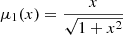 , and μ2 is transcendental.
3.2. MOND modified inertia
For spherical matter distributions, S = 0 (Bekenstein & Milgrom 1984), and it follows that in this special case the Newtonian and MOND (gMI) accelerations are related as
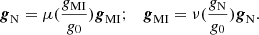 (7)
(7)
These relations with S = 0 also hold in so-called MOND MI models (Milgrom 1983) for any matter distributions. We therefore denote the MOND acceleration as gMI in this case. The acceleration gMI is generally not derivable from a potential as gM defined via Eq. (4), but MOND MI is often used for comparing MOND with rotation curve data irrespective of the distinction between MOND MI and MOND MG. However, as seen above, the g2-space geometry of the two are distinctly different.
Since the function xμ(x) is monotonic, the function gMI(gN) is one-to-one. Then, since the Newtonian acceleration, gN(r), goes to zero for both large and small radii, the g2-space curves, 𝒞, of MOND MI are closed curves with zero area. They are universally neutral geometries (i.e., independent of the underlying baryonic matter distribution and independent of the details of the interpolation function) according to the classification of Table 1 2.
3.3. The deep MONDian regimes at large and small radii
At large radii the solenoidal field, S, in Eq. (5) vanishes faster than the Newtonian acceleration, gN, and so can be neglected. More precisely, the unit-less Newtonian acceleration y = gN/g0 falls off as y ∼ 1/r2, while the solenoidal field, S, vanishes faster than 1/r3, as shown in Bekenstein & Milgrom (1984). Since the inverse interpolation function in the deep MONDian limit y → 0 behaves as ν(y)→y−1/2, the large radius limit of the MOND acceleration is related to the Newtonian as
 (8)
(8)
The g2-space curves and rotation speed curves of MOND MI and MOND MG therefore always coincide at large radii. This is exemplified in the top panel of Fig. 1, where all curves coincide at large radii, corresponding to the gN → 0 parts of the 𝒞+ curve segments (the upper curve segments).
3.3.1. Analytical approximations
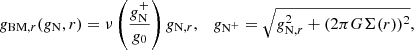
To study the deep MONDian limit y → 0 at small radii, it is instructive to consider an analytic approximation to MOND MG for infinitely thin discs. In particular, we considered an exponential disc with a surface mass density Σ(r) = Σ0e−r/rd. In this case, an approximate expression for the resulting centripetal acceleration gBM, r in MOND MG was given by Brada and Milgrom in Brada & Milgrom (1994). Taking Eq. (7) as an approximation for the MOND MG acceleration outside the disc and then taking into account the discontinuity of the z component of the acceleration inside the disc, one finds the radial acceleration in the plane of the infinitely thin disc:
 (9)
(9)
where gN+ is the total acceleration in the disc, which includes the discontinuity in the z component by taking the limit z → 0+ from the upper half of the plane. Given the limiting behaviour of the density Σ(r) at large and small radii, we find the centripetal acceleration in the two deep MONDian regimes to be
 (10)
(10)
At large radii, this MOND MG approximation coincides with MOND MI, as it should, while at small radii it is reduced by a factor  relative to MOND MI. In the deep MONDian regime at small radii, the MOND and Newtonian accelerations are linearly related, as opposed to the square root relation in the deep MONDian regime at large radii. We show this MOND MG approximation in Fig. 1 as the dotted acceleration (left panel) and speed curves (right panel) and in Fig. 3 as the dotted black curve. The square root and linear behaviour of gBM, r as a function of gN, r in the deep MONDian regimes at small and large radii, respectively, are clearly seen in the figures. It follows that, in this approximation, MOND MG curves are cored with rtot > rN, 𝒞+ > 𝒞−, and 𝒜(𝒞) > 0.
It is also possible to start from a spherical potential for which the MOND MG acceleration coincides with the MOND MI exactly. By adding an axisymmetric perturbation, one can compute the solenoidal field, S, as a function of this perturbation. This is done in Ciotti et al. (2006). We now discuss how the cored geometry of MOND MG arises beyond the infinitely thin disc approximation or the approximation of a nearly spherical mass distribution.
3.3.2. Quasi-linear MOND modified gravity
Before solving the full MOND MG geometries, it is also instructive to consider QUMOND, the quasi-linear version of MOND MG (Milgrom 2010), to see the origin of the cored geometry. The QUMOND acceleration, gQM, is obtained by starting from the (pristine) MOND MI acceleration, gMI, in the right-hand side of Eq. (7) and then adding a solenoidal field, σ = ∇ × A, to enforce that the resulting QUMOND acceleration, gQM, has zero curl. This ensures that the QUMOND acceleration is derivable from a potential:
 (11)
(11)
where the curl of σ follows from the requirement ∇ × gQM = 0 such that gQM = −∇ψQM. This allows us to determine ∇ × σ straightforwardly in terms of the Newtonian potential.
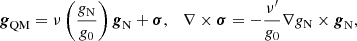
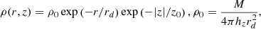
Due to the axisymmetry of the matter distribution, the curl ∇ × σ is purely in the azimuthal direction, and, using the second identity in Eq. (11), we can also determine the sign of ∇ × σ in the azimuthal direction to be negative. This is shown in Fig. 2 for a Miyamoto-Nagai (MN) potential, which is given in Eq. (13) and reviewed in Sect. 3.4. The scale length (a), scale height (b), and mass scale (M) of the MN model used in the figure are a = 1, b = 0.5, and M = 1 (bottom left). The negative sign arises as follows: For z ≥ 0, the gradient ∇gN is dominantly in the z direction for a non-spherical, axisymmetric mass distribution (it is zero in the plane by symmetry unless the disc is infinitely thin), while gN is dominantly in the negative r direction. This is illustrated for the MN model in Fig. 2 in the left and middle panels, respectively. It is particularly clear at the line of maximum radial acceleration, ∂rgN = 0, near r = 1.1, where ∇gN points entirely in the positive z direction and gN is dominantly in the negative radial direction. Then, since ν′ < 0 in the MONDian regimes at small and large radii, we have that ∇ × σ is in the negative azimuthal direction, as seen in the right-hand panel of the figure, and, consequently, σ circulates in the anticlockwise direction in the (r, z) plane.
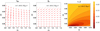 |
Fig. 2. Gradient of the norm of the Newtonian acceleration, ∇gN (left panel), the Newtonian acceleration vector, gN (middle panel), and the curl of the solenoidal field, ∇ × σ (right panel), in QUMOND for an MN disc model with mass parameter MMN = 1, scale height b = 0.5, and scale length a = 1. From the sign of ∇ × σ, we infer that the centripetal component of the curl acceleration is in the opposite direction of the Newtonian acceleration vector, gN, in the disc near z = 0. |
At large radii σ is negligible, but at small radii the radial component of gQM is reduced as compared to the radial component of gMI because the radial acceleration from the solenoidal field, σ, is in the opposite direction to the Newtonian acceleration, gN. It follows, using the classification of Table 1, that the QUMOND MG geometries are cored.
3.3.3. Solenoidal field in MOND modified gravity
The arguments above for QUMOND may also be applied to the solenoidal field, S, of the Bekenstein-Milgrom MOND MG (note the opposite sign convention!). The curl ∇ × S may be expressed from either of the two identities in Eq. (12), using ∇ × gN = ∇ × gM = 0, as
 (12)
(12)
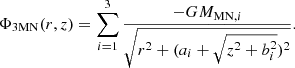
Due to the axisymmetry, the curl, ∇ × S, is again purely in the azimuthal direction. We can argue that the sign of ∇ × S is in the negative azimuthal direction such that S circulates in the anticlockwise direction by repeating the arguments for QUMOND: At large radii, the solenoidal field is negligible, and as we move towards smaller radii we approximate q ≃ gN in the above formula and repeat the arguments above for QUMOND (i.e. near the z = 0 plane the radial acceleration is reduced as compared to that in MOND MI). It follows that the MOND MG geometries are cored, as in QUMOND, using the classification of Table 1. Example numerical solutions of Eq. (4), using the N-MODY code, are shown in the top-left panel of Fig. 3 (coloured dotted curves) as a function of the parameter b, which controls the departure from the spherical limit. We now discuss these numerical solutions.
 |
Fig. 3. Top-left panel: centripetal acceleration curves in g2 space of MOND MI (solid grey curve) and MOND MG in the Brada-Milgrom approximation (black dotted curve) with acceleration scale g0 = 1.2 × 10⁻¹⁰ m s−2 for a 3MN model of an infinitely thin exponential disc galaxy with M = 1.2 × 10¹⁰ M⊙ and a scale length of rd = 3.5 kpc. The 3MN parameters are given in the appendix. The dotted coloured curves are the full MOND MG solution of the same model but with the scale height parameter of the 3MN model varied: b = 3 (green), b = 1 (red), and b = 0.3 (blue) (b → 0 is the disc limit, and b → ∞ is the spherical limit). Finally, the solid orange line gives the purely Newtonian acceleration. Top-right panel: corresponding rotation curves showing the full MOND MG solution only for b = 0.3. Bottom-left panel: corresponding curl field S for the b = 3 case, showing how the curl field at z = 0 is in the opposite direction to the Newtonian one and how it reduces the radial MOND MG acceleration compared to the MOND MI. Bottom-right panel: difference in curl fields for the most disc-like (b = 0.3) and most spherical (b = 3) parameter values, showing that the solenoidal field reduces the radial MOND MG acceleration in the z = 0 plane most for the most disc-like mass distributions. |
3.4. Numerical solutions of MOND modified gravity
In order to study numerical solutions of the full MOND MG geometries in g2 space, it is useful to consider MN potentials, which interpolate between axisymmetric potentials and spherical potentials. The MN potential, ΦMN, is given by
 (13)
(13)
where MMN is a mass parameter, b is the vertical scale height, and a is the radial scale length (Miyamoto & Nagai 1975). In the limit a = 0, the potential is spherically symmetric and reduces to the Plummer potential. For a ≠ 0 the potential is axisymmetric (and symmetric about the z = 0 plane), and in the limit b = 0 the potential reduces to the potential of an infinitely thin Kuzmin disc, for which the MOND MG solution is known exactly.
However, instead of a single MN model, we used a sum of three Miyamoto-Nagai potentials (3MN models), which can be used to approximate the potential of both thick and thin exponential discs (Smith et al. 2015), with densities of the form
 (14)
(14)
where rd is the radial scale length and z0 is the vertical scale length. This allows us to compare numerical solutions of MOND MG to both the Brada-Milgrom approximation for infinitely thin exponential discs and MOND MI in the spherical limit. The 3MN potentials we used are therefore of the form:
 (15)
(15)
We discuss details of the 3MN approximation in the appendix.
As an example, we started from an infinitely thin exponential disc galaxy with a mass of M = 1.2 × 10¹⁰ M⊙ and a scale length of rd = 3.5 kpc and took g0 = 1.2 × 10⁻¹⁰ m s−2. The corresponding 3MN model parameters, M3MN, b = 0, ai, Mi, are given in the appendix and are used to compute the MOND MI gMI curve (solid grey line) and MOND MG in the Brada-Milgrom approximation, gBM (dotted black line), in the top-left panel of Fig. 3. By dialling the parameter b up, we can make the mass distribution more spherical, with a/b → 0 the spherical limit (corresponding to increasing the scale height, z0, in the thick exponential disc above).
The coloured dotted curves show the full solution of the MOND MG curve, using the static solver of the N-MODY code for the 3MN models with increasing values of b from b = 0.3 (blue), to b = 1 (orange), to b = 3 (green).
The figure demonstrates the properties discussed previously: The MOND MI and MOND MG curves coincide at large radii, but the MOND MG curves are more cored at small radii and the core grows in proportion to the departure from spherical symmetry (as measured by the ratio a/b here) towards the Brada-Milgrom approximation in the thin disc limit a/b → ∞. We show the rotation speed curves corresponding the MOND MI and Brada-Milgrom curves along with the full numerical solution for b = 0.3 in the top-right panel. Finally, it is seen how the approach to zero acceleration of the curves follows the radial limiting behaviour given in Eq. (10). We also note that increasing the mass of the disc, such that the accelerations reach the Newtonian regime, simply means the curves are stretched and the core effect at small radii is less pronounced.
In the bottom-left panel we show the corresponding solenoidal field, S, for the b = 3 example. The curl field indeed circulates in the anticlockwise direction. Finally, in the bottom-right panel of the figure, we show that the difference between the b = 0.3 and b = 3 curl fields is positive near z = 0; therefore, the least spherical potential leads to the biggest curl field along the z = 0 plane and thus the biggest core effect. We can therefore take the Brada-Milgrom approximation as a good approximation of MOND MG for thin discs. For more spherical mass distributions, the Brada-Milgrom will overestimate the core, so for a given galaxy we can take the Brada-Milgrom formula and apply it to a thin disc of equivalent mass to get an upper limit on the core produced by MOND MG in the galaxy.
In summary, we have shown that MOND MG leads to cored g2-space geometries (and corresponding rotation curves) for isolated galaxies and that the core effect is then smallest for the most spherical systems, for example dwarf spheroidals. MOND MI, which is also the limit of MOND MG for fully spherical baryonic mass distributions, leads to neutral geometries.
4. MOND models and SPARC galaxy data in g2 space
We now compare MOND model acceleration curves to data from the SPARC galaxy database (Lelli et al. 2016). We focus on galaxies that exhibit cuspy and cored geometries, respectively.
The geometry of MOND MG is cored relative to MOND MI. Therefore, the (simpler) fits of MOND MI to cuspy galaxies provide an upper limit on the goodness of fit for MOND MG to such galaxies. Conversely from Fig. 3, we can use the Brada-Milgrom approximation as an upper limit on how cored MOND MG can be (i.e., how big the enclosed area 𝒜(C) is). Our data analysis below follows that in Frandsen & Petersen (2018) and is detailed in Appendix A.
4.1. Cored and cuspy SPARC galaxies
In the top-left panel of Fig. 4, we show galaxies from SPARC with cored g2-space geometries (colour legend in the figure identifies the individual galaxies) along with the MI model with the interpolation functions in Eq. (6) and with the best-fit value g0 = 1.2 × 10⁻¹⁰ m s−2 from Lelli et al. (2016) (solid and dashed grey lines). The galaxies were selected as cored only by requiring robs, G > rbar, G and by having a large  value for the fit of data from each galaxy to the MOND MI curve in Eq. (6). Below, we discuss the fits in more detail. In the top-right panel we show the same for galaxies with cuspy g2-space geometries, selected as cuspy only by requiring robs, G < rbar, G and, again, by having a large
  for the fit of the data from each galaxy to the curve in Eq. (6).
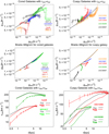 |
Fig. 4. Top-left panel: acceleration curves of galaxies from SPARC in g2 space with cored geometry robs > rbar. Top-right panel: same but for cuspy galaxies with robs < rbar. Also shown in both panels are the MOND MI curves for the two interpolation functions considered in Eq. (6). Middle-left panel: corresponding model curves for the cored galaxies from MOND MG curves using the Brada-Milgrom approximation with the gbar and surface density Σ(r) values from SPARC. Middle-right panel: same as left but for the cuspy galaxies. For reference, the MOND MI curve is also shown again. Bottom-left panel: corresponding rotation speed curve data for two of the cored galaxies, compared to the MOND MI and MOND MG curves. Bottom-right panel: same as left but for two cuspy galaxies |
In the middle row of panels we show the predicted MOND MG curves of the same cored and cuspy galaxies along with the MOND MI curves for reference. We obtained the MOND MG curves using the Brada-Milgrom approximation in Eq. (9), with gN replaced by the data gbar(rj, G) and with Σ(r) replaced by the disc surface densities Σ(rj, G) from SPARC.
It is visually clear that the MOND MG curves yield poor fits to both the cored and cuspy galaxies, as we quantify further below. For the cuspy galaxies the MOND MG is, by nature of its cored geometry, a worse description than MOND MI. For the cored galaxies, the MOND MG curves are everywhere too close to the MOND MI limit to describe the cored geometry of the data. In particular, the MOND MG curves are more cored for the cuspy galaxies than they are for the cored ones because the latter have larger stellar surface mass densities.
In the bottom row of panels we show the corresponding rotation speed curves for two of the cored and two of the cuspy galaxies compared to the predictions from MOND MI and the Brada-Milgrom approximation of MOND MG.
In Fig. 5 we show the distribution of normalized residuals, R(rj, G), from Eq. (A.3) of the SPARC data after quality cuts and the δvobs/vobs < 0.1 cut employed in McGaugh et al. (2016), Lelli et al. (2017), and Lelli et al. (2016) with respect to the MOND MI prediction with g0 = 1.2 × 10⁻¹⁰ m s−2. The grey histograms, highlighted with black dots in the middle of the bins, show the residuals of all SPARC data points at large radii (i.e., with rj, G > rbar, G). These points are seen to follow the Gaussian of unit width superimposed on the figure, as expected of a good fit. The left panel also shows the residuals of data at small radii, meaning rj, G ≤ rbar, G from the (cored) galaxies with robs, G > rbar, G (red histogram). These residuals are not Gaussian but skewed towards large negative residuals, which is consistent with these points being below the MOND MI prediction in general, as is the case for our example galaxies. This is also what MOND MG would in general predict they should be; however, for our examples in Fig. 4, the specific cores of MOND MG do not match the data well. In the right panel we also show the residuals of data at small radii, rj, G ≤ rbar, G, from (cuspy) galaxies with robs, G < rbar, G (blue histogram). These residuals are skewed towards large positive residuals, consistent with these points lying above the MOND MI predictions and therefore also above the MOND MG predictions in g2 space.
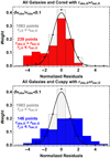 |
Fig. 5. Top panel: distribution of the normalized residuals R(rj, G) in Eq. (A.3) of SPARC data with respect to MOND MI with g0 = 1.2 × 10⁻¹⁰ m s−2. The grey histograms with black dots at each bin top shown on both panels are the 1983 SPARC data points at large radii, i.e., rj, G > rbar, G, after imposing the basic quality criteria and the δvobs/vobs < 0.1 cut employed in McGaugh et al. (2016), Lelli et al. (2017), and Lelli et al. (2016). Also shown in the top panel are normalized residuals of data points at small radii, rj, G ≤ rbar, G, from the (cored) galaxies only with robs, G > rbar, G (red histogram). Bottom panel: points at small radii, rj, G < rbar, G, from (cuspy) galaxies only with robs, G < rbar, G (cuspy; blue histogram). |
We note that seven of the galaxies in SPARC with steeply rising (cuspy) rotation curves are starburst dwarf galaxies, for which data may not faithfully represent the underlying gravitational potential, as discussed in Read et al. (2016) and Santos-Santos et al. (2018). However, some of those galaxies are eliminated by the data quality cut employed here, and they are not among the galaxies presented in Fig. 4.
4.2. Model fits to data
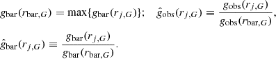
To reduce systematic uncertainties in the data before performing quantitative fits of MOND to the galaxies in Fig. 4, we defined the radius of maximum baryonic acceleration in the data (in analogy with the model rN above) and acceleration ratios as:
 (16)
(16)
These ratios, introduced in Frandsen & Petersen (2018), eliminate the systematic uncertainties on galactic distance and inclination angle for gobs, and they significantly reduce the systematic error from gas measurements and mass to-light ratios for gbar. The resulting uncertainties,  and
and  , are given in Frandsen & Petersen (2018) and reproduced in Appendix B. Using the acceleration ratios, we constructed the
  of each galaxy compared to the model acceleration,
 (17)
(17)
where  is the MOND model prediction with the data point
  as input, and the inverse variance matrix,
  , given in in Appendix B, takes into account the systematic uncertainty from the normalization point common to all acceleration ratios within a single galaxy. We neglected the uncertainties in
  which are small compared to those in
  for most data points, as seen in Figs. 7 and 6, where the acceleration ratios with errors are shown.
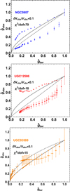 |
Fig. 6. Acceleration ratio curves |


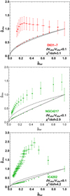 |
Fig. 7.
|


4.2.1. Cuspy SPARC galaxies
We first studied three of the cuspy galaxies shown in the top-right panel of Fig. 4. Their corresponding data curves – with errors in the normalized  variables and after imposing the data cut δvobs/vobs < 0.1 used in Lelli et al. (2017) and Lelli et al. (2016) – are shown in Fig. 6. Also shown are the MOND MI curves with g0 = 1.2 × 10⁻¹⁰ m s−2 (solid grey) and with the best-fit value g0, min that minimizes the
  in Eq. (17) (dashed grey). Finally, the MOND MG model curve using the Brada-Milgrom approximation is shown as points without errors in the same colour as the data.
The uncertainties on  are indeed small compared to those on
  for most points. We could therefore compute the
  value for each of these galaxies with respect to MOND using Eq. (17). We give the
  value of MOND MI with g0 = 1.2 × 10⁻¹⁰ m s−2 fixed (McGaugh et al. 2016) in the second row of Table 2 and the minimum
  with the corresponding g0, min value in the third row. As already discussed, and as is clear from the figures, the
  values of MOND MG will be larger or equal to those of MOND MI quoted here.
Acceleration ratio curves  (points with errors) in
  space for three of the cuspy SPARC galaxies.
4.2.2. Cored SPARC galaxies
We next considered fits of MOND to three of the cored galaxies shown in g2 space in the top-left panel of Fig. 4. The corresponding acceleration ratio curves are shown in Fig. 7. The  values of these galaxies with respect to MOND MI, analogous to those above for cuspy galaxies, are listed in Table 3.
χ2 values for fits of MOND MI to cored galaxy examples.
Again, we find large  values for the fits to MOND MI, and, given the very little difference between this and MOND MG seen in the figures, we can also take these values for MOND MG.
As summarized in Tables 2 and 3, the MOND fits to individual cuspy and cored galaxies return large χ2 values and a significant variation in g0. These best-fit values of g0 deviate considerably from the value g0 = 1.2 × 10⁻¹⁰ m s−2, which was found in Lelli et al. (2017) as a best fit to the entire SPARC dataset.
These deviations can be understood following the discussion in Petersen & Frandsen (2020): At large radii, MOND MI and MOND MG are indistinguishable, as shown in Fig. 3. (This is so since MOND MG reduces to MI in the spherical limit, which is approximately valid at large distances). They both predict  at these radii, and we should expect the models to reproduce data well by virtue of their original construction. By contrast, MOND MI and MOND MG differ distinctly at radii r ≲ rbar, where the difference between cuspy and cored acceleration curve geometries particularly manifests itself (it is also where the difference between cuspy and cored DM density profiles manifests itself).
The SPARC database is dominated by points at large radii, r > rbar (the 1983 points in grey in Fig. 5), which are indeed in good agreement with both MOND MI and MOND MG. Compared to MG, there are 385 points at small radii, r ≤ rbar (the red and blue points shown in Fig. 5 ), which are in poor agreement with MOND; Fig. 5 displays the large non-Gaussian residuals of these data points with respect to MOND MI with g0 = 1.2 × 10⁻¹⁰ m s−2.
Since most of the data points are at large radii, r > rbar, in SPARC, a fit to all these data points that does not retain radial information, as the one in Lelli et al. (2017), will also mostly test the behaviour of acceleration curves at large radii. However, radial information from each galaxy is needed in order to fully test any model and to distinguish between different models – for example, by simply analysing individual galaxies, as we do in this study.
5. Summary
In this paper we have provided and employed a new definition of cuspy and cored galactic acceleration curve geometries that is applicable to both DM and MOND models of missing mass. Cuspy and cored acceleration curves are defined relative to the curves of MOND MI, which we take as a neutral reference, and the classification in the space of baryonic and total accelerations (g2 space) is that proposed in Frandsen & Petersen (2018). This new definition is summarized in Table 1, illustrated in Fig. 1, and used throughout, unless otherwise stated.
Examples of cored and cuspy acceleration curves in g2 space, and corresponding rotation speed curves, from the SPARC database are shown in the top and bottom panels of Fig. 4. We fit MOND MI and MOND MG to some of these galaxies in Figs. 6 and 7, with the intrinsic MOND acceleration scale g0, defined in Eq. (4), as fit parameter. To eliminate systematic uncertainties from galaxy distance and inclination angle and to reduce the systematic uncertainty from mass-to-light ratios, the fit is performed on ratios of accelerations  and
and  defined in Eq. (16). As summarized in Tables 2 and 3, the fits return large χ2 values and significant variation in the best-fit values of g0 between different galaxies. Also, these best-fit values of g0 deviate considerably from the value g0 = 1.2 × 10⁻¹⁰ m s−2 that was found in Lelli et al. (2017) as a best fit to the entire SPARC dataset. These deviations are visually clear from Fig. 4 and are in line with our previous finding: that the neutral geometry of MOND MI, specifically the prediction gtot(rtot) = gtot(rN), is in tension with the full SPARC dataset of circa 150 galaxies Frandsen & Petersen (2018), independent of the MOND interpolation function chosen.
The cored acceleration curves from MOND MG models are most pronounced for galaxies with the most disc-like baryonic matter distribution, and, in the limit of spherical distributions, they reduce to the neutral curves of MOND MI with the functional relation gtot = gtot(gN). This is shown in Fig. 3 and discussed in Sect. 3. The cored and neutral curves of MOND can be contrasted with, for example, the cuspy curves from NFW DM density profiles that arise in N-body simulations of DM structure formation without baryons.
Based on our results and our new definition of cuspy, cored, and neutral acceleration curve geometries, we have elucidated an observational challenge for MOND, which we refer to as the cusp-core challenge: MOND MG leads to cored acceleration curves for isolated galaxies as a consequence of the solenoidal field, S, arising from the modified Poisson equation given in Eq. (5). MOND MI leads to neutral acceleration curves for isolated galaxies as a consequence of the one-to-one functional relationship between the Newtonian and MOND MI accelerations given in Eq. (7). In particular, neither allows for cuspy acceleration curves. By contrast, as illustrated in the top panels of Fig. 4, galactic acceleration curves inferred from observations display a diversity of cored and neutral as well as cuspy acceleration curve geometries.
This cusp-core challenge we have identified for MOND is analogous to – but essentially the inverse of – the DM cusp-core problem (Flores & Primack 1994), in the sense that DM-only N-body simulations lead to NFW-like cuspy DM density profiles (Navarro et al. 1996). By contrast, a diversity of cored and cuspy density profiles are inferred from observations.
Baryonic feedback from supernovae can change cuspy DM profiles into cored ones in some cases (Read & Gilmore 2005; Teyssier et al. 2013; Di Cintio et al. 2014). In the future, it would be interesting to investigate whether, for example, the external field effect in MOND or a radial dependence of the mass-to-light ratios impact and potentially alleviate the problem posed by the cusp-core challenge for MOND.
As in Frandsen & Petersen (2018), we used gtot for total predicted model accelerations and gobs for the total observed. Similarly, we used gN for the Newtonian accelerations from baryons in a given model and gbar for the same inferred quantity from data.
Acknowledgments
We thank J. Read, W.-C. Huang and J. Smirnov for discussions and comments on the draft. The authors acknowledge partial funding from The Council For Independent Research, grant number DFF 6108-00623. The CP3-Origins center is partially funded by the Danish National Research Foundation, grant number DNRF90.
References
- Banik, I., Milgrom, M., & Zhao, H. 2018, ArXiv e-prints [arXiv:1808.10545] [Google Scholar]
- Begeman, K. G., Broeils, A. H., & Sanders, R. H. 1991, MNRAS, 249, 523 [Google Scholar]
- Bekenstein, J. D. 2004, Phys. Rev. D, 70, 083509 [Erratum: Phys. Rev. D, 71, 069901(2005)] [Google Scholar]
- Bekenstein, J., & Milgrom, M. 1984, ApJ, 286, 7 [NASA ADS] [CrossRef] [Google Scholar]
- Bosma, A. 1981, AJ, 86, 1825 [NASA ADS] [CrossRef] [Google Scholar]
- Brada, R., & Milgrom, M. 1994, ArXiv e-prints [arXiv:astro-ph/9407071] [Google Scholar]
- Ciotti, L., Londrillo, P., & Nipoti, C. 2006, ApJ, 640, 741 [NASA ADS] [CrossRef] [Google Scholar]
- Clowe, D., Bradac, M., Gonzalez, A. H., et al. 2006, ApJ, 648, L109 [NASA ADS] [CrossRef] [Google Scholar]
- Di Cintio, A., Brook, C. B., Maccio, A. V., et al. 2014, MNRAS, 437, 415 [NASA ADS] [CrossRef] [Google Scholar]
- Dodelson, S. 2011, Int. J. Mod. Phys. D, 20, 2749 [NASA ADS] [CrossRef] [Google Scholar]
- Dodelson, S., & Liguori, M. 2006, Phys. Rev. Lett., 97, 231301 [NASA ADS] [CrossRef] [Google Scholar]
- Famaey, B., & McGaugh, S. 2012, Liv. Rev. Rel., 15, 10 [NASA ADS] [CrossRef] [Google Scholar]
- Flores, R. A., & Primack, J. R. 1994, ApJ, 427, L1 [NASA ADS] [CrossRef] [Google Scholar]
- Frandsen, M. T., & Petersen, J. 2018, ArXiv eprints [arXiv:1805.10706] [Google Scholar]
- Gentile, G., Famaey, B., & de Blok, W. J. G. 2011, A&A, 527, A76 [NASA ADS] [CrossRef] [EDP Sciences] [Google Scholar]
- Lee, B. W., & Weinberg, S. 1977, Phys. Rev. Lett., 39, 165, [,183(1977)] [NASA ADS] [CrossRef] [Google Scholar]
- Lelli, F., McGaugh, S. S., & Schombert, J. M. 2016, AJ, 152, 157 [Google Scholar]
- Lelli, F., McGaugh, S. S., Schombert, J. M., & Pawlowski, M. S. 2017, ApJ, 836, 152 [Google Scholar]
- Li, P., Lelli, F., McGaugh, S., & Schormbert, J. 2018, A&A, 615, A3 [NASA ADS] [CrossRef] [EDP Sciences] [Google Scholar]
- McGaugh, S. 2008, ApJ, 683, 137 [NASA ADS] [CrossRef] [Google Scholar]
- McGaugh, S. S., Schombert, J. M., Bothun, G. D., & de Blok, W. J. G. 2000, ApJ, 533, L99 [Google Scholar]
- McGaugh, S., Lelli, F., & Schombert, J. 2016, Phys. Rev. Lett., 117, 201101 [NASA ADS] [CrossRef] [Google Scholar]
- Milgrom, M. 1983, ApJ, 270, 365 [Google Scholar]
- Milgrom, M. 2010, MNRAS, 403, 886 [NASA ADS] [CrossRef] [Google Scholar]
- Milgrom, M., & Sanders, R. H. 2008, ApJ, 678, 131 [NASA ADS] [CrossRef] [Google Scholar]
- Miyamoto, M., & Nagai, R. 1975, PASJ, 27, 533 [NASA ADS] [Google Scholar]
- Navarro, J. F., Frenk, C. S., & White, S. D. M. 1996, ApJ, 462, 563 [Google Scholar]
- Navarro, J. F., Ludlow, A., Springel, V., et al. 2010, MNRAS, 402, 21 [Google Scholar]
- Oman, K. A., Navarro, J. F., Fattahi, A., et al. 2015, MNRAS, 452, 3650 [CrossRef] [Google Scholar]
- Orear, J. 1982, Am. J. Phys., 50, 912 [Google Scholar]
- Petersen, J., & Frandsen, M. T. 2020, MNRAS, 496, 1077 [NASA ADS] [CrossRef] [Google Scholar]
- Read, J. I., & Gilmore, G. 2005, MNRAS, 356, 107 [NASA ADS] [CrossRef] [Google Scholar]
- Read, J. I., Iorio, G., Agertz, O., & Fraternali, F. 2016, MNRAS, 462, 3628 [NASA ADS] [CrossRef] [Google Scholar]
- Rubin, V. C., & Ford, W. K., Jr 1970, ApJ, 159, 379 [NASA ADS] [CrossRef] [Google Scholar]
- Rubin, V. C., Thonnard, N., & Ford, W. K., Jr 1980, ApJ, 238, 471 [NASA ADS] [CrossRef] [Google Scholar]
- Sanders, R. H. 2003, MNRAS, 342, 901 [NASA ADS] [CrossRef] [Google Scholar]
- Sanders, R. H., & McGaugh, S. S. 2002, ARA&A, 40, 263 [NASA ADS] [CrossRef] [Google Scholar]
- Santos-Santos, I. M., Di Cintio, A., Brook, C. B., et al. 2018, MNRAS, 473, 4392 [NASA ADS] [CrossRef] [Google Scholar]
- Skordis, C., Mota, D. F., Ferreira, P. G., & Boehm, C. 2006, Phys. Rev. Lett., 96, 011301 [CrossRef] [Google Scholar]
- Smith, R., Flynn, C., Candlish, G. N., Fellhauer, M., & Gibson, B. K. 2015, MNRAS, 448, 2934 [Google Scholar]
- Steigman, G., & Turner, M. S. 1985, Nucl. Phys. B, 253, 375 [NASA ADS] [CrossRef] [Google Scholar]
- Stump, D., Pumplin, J., Brock, R., et al. 2001, Phys. Rev. D, 65, 014012 [NASA ADS] [CrossRef] [Google Scholar]
- Teyssier, R., Pontzen, A., Dubois, Y., & Read, J. 2013, MNRAS, 429, 3068 [NASA ADS] [CrossRef] [Google Scholar]
- Tully, R. B., & Fisher, J. R. 1977, A&A, 54, 661 [NASA ADS] [Google Scholar]
- Zwicky, F. 1933, Helv. Phys. Acta, 6, 110 [Gen. Rel. Grav. 41, 207 (2009)] [NASA ADS] [Google Scholar]
Appendix A: Galaxy data analysis
The SPARC database provides the observed rotational velocities, vobs(rj, G), as well as the inferred contributions to the baryonic velocity from the disc, bulge, and gas in the galaxy, vdisc(rj, G), vbul(rj, G), and vgas(rj, G), with rj, G the jth measured radius in the galaxy, G. The accelerations gobs(rj, G) and gbar(rj, G) are then
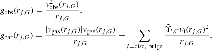 (A.1)
(A.1)
where  and
and  are unit-less mass-to-light ratio rescaling factors. They are included following McGaugh et al. (2016), Lelli et al. (2017), Lelli et al. (2016), and Li et al. (2018) because the speed data, vi(rj, G), listed in the SPARC database are all quoted assuming reference mass-to-light ratios equal to that of the Sun, Υi, G = M⊙/L⊙. Following McGaugh et al. (2016), Lelli et al. (2017), Lelli et al. (2016), and Li et al. (2018), we take the central values,
  and
and  , including a 25% relative uncertainty on both,
  .
.
We note the absolute value on vgas. This appears because for some galaxies in the SPARC database vgas is reconstructed as negative in the innermost regions of the galaxies. This happens when the gas distribution has a large central depression and the gravitational force from the material in the outer regions is stronger than the force from the material in the inner regions. In this case, the gas acts to reduce rather than enhance the total centripetal acceleration, and this is taken into account in the accelerations computed from SPARC data via negative vgas values for these radii as discussed in Lelli et al. (2016). The galaxy UGC03580, shown in Figs. 4 and 6, and the galaxy UGC08286, shown in Fig. 4 only, has such negative vgas values. All the other galaxies used here do not.
The SPARC database also provides the corresponding (random) uncertainties δvobs(rj, G), as well as the uncertainties δiG and δDG on the galaxy inclination angle, iG, and distance, DG. Following Lelli et al. (2017), we further adopted a 10% uncertainty on the HI flux calibration, which translated into a 10% uncertainty on the gas accelerations (i.e. δggas(rj, G) = 0.1ggas(rj, G)). From these uncertainty contributions, we can compute the full δgbar, δgobs uncertainties:
![Mathematical equation: $$ \begin{aligned} \delta {g_{\rm obs}}(r_{j,G})&= g_{\rm obs}(r_{j,G}) \sqrt{\bigg [\dfrac{2\delta {v_{\rm obs}} (r_{j,G}) }{v_{\rm obs}(r_{j,G}) }\bigg ]^{2} + \bigg [\dfrac{2\delta i_G}{\tan (i_G)}\bigg ]^{2} + \bigg [\dfrac{\delta D_G}{D_G}\bigg ]^{2}}, \nonumber \\ \delta {g_{\rm bar}}(r_{j,G})&= g_{bar}(r_{j,G})\sqrt{\bigg (\frac{\delta g_{\rm gas}(r_{j,G})}{g_{\rm bar}(r_{j,G})}\bigg )^2 + \sum _{k=disc,bulge}\bigg (\frac{v_{k}^2(r_{j,G}) \delta \Upsilon _{k,G}}{v_{bar}^2(r_{j,G})}\bigg )^2 }, \end{aligned} $$](/articles/aa/full_html/2021/12/aa40189-20/aa40189-20-eq65.gif) (A.2)
(A.2)
where we note that the inferred gbar(rj, G) are independent of distance, DG, and inclination angle, iG (Li et al. 2018). We treat the uncertainties δvobs as random Gaussian-distributed uncertainties for each data point, while the remaining uncertainties, δiG, δDG, δΥdisc, bulge, G, and δggas(rj, G), are systematic within each galaxy, meaning they rescale all data points within a given galaxy in one direction.
The normalized residuals that enter into the χ2 function, taking the errors in both the observed and baryonic accelerations into account, can be approximated as (Orear 1982)
 (A.3)
(A.3)
where  is the derivative with respect to the baryonic acceleration.
Appendix B: Uncertainties on acceleration ratios and variance matrix
The uncertainty contributions to  and
and  following from Eq. (A.1), are
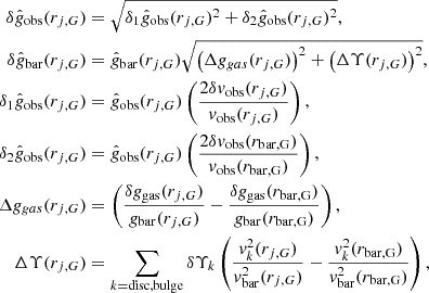 (B.1)
(B.1)
where we have separated the uncertainty contribution  which is random for all points within a galaxy, and the contribution from the normalization
  which is a systematic for all data points within a single galaxy. With these ratios, we constructed the χ2 of each galaxy compared to the model acceleration:
 (B.2)
(B.2)
where  is the MOND model prediction with the data point
  as input, and the inverse variance matrix (e.g. Stump et al. 2001) is
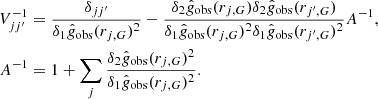 (B.3)
(B.3)
The second term in  comes from the systematic uncertainties
  introduced due to the common normalization point. We neglected the uncertainties in
  , which are small compared to those in
  for most data points, as seen in Figs. 7 and 6.
Appendix C: 3MN model
Parameters used for the 3MN model.
As discussed in the main text, the sum of three MN discs can be used to model an exponential disc profile using the following procedure (Smith et al. 2015). First, the single scale length used in all three potentials, b, is found in terms of the exponential disc scale length, Rd, and scale height, hz, as
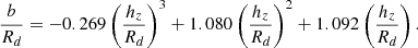 (C.1)
(C.1)
The remaining six parameters, the three mass scale parameters, MMN, 1, MMN, 2, and MMN, 3, and the three scale height parameters, a1, a2, and a3, are found from the equation
 (C.2)
(C.2)
with the numerical parameters ki given in Table C.1
The 3MN models found by this table match the analytical exponential disc < 1.0% out to 4Rd and < 3.3% out to 10Rd (Smith et al. 2015). For our purposes, the 3MN model is convenient because we can use it to explicitly interpolate between spherical and disc-like matter distributions.
All Tables
Geometric characteristics of cuspy, neutral, and cored geometries of rotation acceleration curves.
Acceleration ratio curves (points with errors) in space for three of the cuspy SPARC galaxies.
All Figures
|
Fig. 1. Top panel: centripetal acceleration curves in g2 space with the quantities rtot, rN, and 𝒞±, used for classification in Table 1, shown. The solid grey line shows a MOND MI curve with the radius of maximum baryonic acceleration and maximum total acceleration rN = rtot indicated. Also, the curve segments 𝒞+ and 𝒞− coincide, so the curve area is 𝒜(𝒞) = 0. The dotted grey and dotted black curves show the 𝒞± curve segments of a MOND MG curve, using the Brada-Milgrom approximation in Eq. (9), with rtot > rN and 𝒜(𝒞) > 0. For both, the baryonic matter is an infinitely thin exponential disc, Σ(r) = Σ0e−r/rd. The arrow indicates the direction of increasing radius along the curve. Bottom panel: corresponding rotation curves. |
| In the text | |
|
Fig. 2. Gradient of the norm of the Newtonian acceleration, ∇gN (left panel), the Newtonian acceleration vector, gN (middle panel), and the curl of the solenoidal field, ∇ × σ (right panel), in QUMOND for an MN disc model with mass parameter MMN = 1, scale height b = 0.5, and scale length a = 1. From the sign of ∇ × σ, we infer that the centripetal component of the curl acceleration is in the opposite direction of the Newtonian acceleration vector, gN, in the disc near z = 0. |
| In the text | |
|
Fig. 3. Top-left panel: centripetal acceleration curves in g2 space of MOND MI (solid grey curve) and MOND MG in the Brada-Milgrom approximation (black dotted curve) with acceleration scale g0 = 1.2 × 10⁻¹⁰ m s−2 for a 3MN model of an infinitely thin exponential disc galaxy with M = 1.2 × 10¹⁰ M⊙ and a scale length of rd = 3.5 kpc. The 3MN parameters are given in the appendix. The dotted coloured curves are the full MOND MG solution of the same model but with the scale height parameter of the 3MN model varied: b = 3 (green), b = 1 (red), and b = 0.3 (blue) (b → 0 is the disc limit, and b → ∞ is the spherical limit). Finally, the solid orange line gives the purely Newtonian acceleration. Top-right panel: corresponding rotation curves showing the full MOND MG solution only for b = 0.3. Bottom-left panel: corresponding curl field S for the b = 3 case, showing how the curl field at z = 0 is in the opposite direction to the Newtonian one and how it reduces the radial MOND MG acceleration compared to the MOND MI. Bottom-right panel: difference in curl fields for the most disc-like (b = 0.3) and most spherical (b = 3) parameter values, showing that the solenoidal field reduces the radial MOND MG acceleration in the z = 0 plane most for the most disc-like mass distributions. |
| In the text | |
|
Fig. 4. Top-left panel: acceleration curves of galaxies from SPARC in g2 space with cored geometry robs > rbar. Top-right panel: same but for cuspy galaxies with robs < rbar. Also shown in both panels are the MOND MI curves for the two interpolation functions considered in Eq. (6). Middle-left panel: corresponding model curves for the cored galaxies from MOND MG curves using the Brada-Milgrom approximation with the gbar and surface density Σ(r) values from SPARC. Middle-right panel: same as left but for the cuspy galaxies. For reference, the MOND MI curve is also shown again. Bottom-left panel: corresponding rotation speed curve data for two of the cored galaxies, compared to the MOND MI and MOND MG curves. Bottom-right panel: same as left but for two cuspy galaxies |
| In the text | |
|
Fig. 5. Top panel: distribution of the normalized residuals R(rj, G) in Eq. (A.3) of SPARC data with respect to MOND MI with g0 = 1.2 × 10⁻¹⁰ m s−2. The grey histograms with black dots at each bin top shown on both panels are the 1983 SPARC data points at large radii, i.e., rj, G > rbar, G, after imposing the basic quality criteria and the δvobs/vobs < 0.1 cut employed in McGaugh et al. (2016), Lelli et al. (2017), and Lelli et al. (2016). Also shown in the top panel are normalized residuals of data points at small radii, rj, G ≤ rbar, G, from the (cored) galaxies only with robs, G > rbar, G (red histogram). Bottom panel: points at small radii, rj, G < rbar, G, from (cuspy) galaxies only with robs, G < rbar, G (cuspy; blue histogram). |
| In the text | |
|
Fig. 6. Acceleration ratio curves |
| In the text | |
|
Fig. 7.
|
| In the text | |
Current usage metrics show cumulative count of Article Views (full-text article views including HTML views, PDF and ePub downloads, according to the available data) and Abstracts Views on Vision4Press platform.
Data correspond to usage on the plateform after 2015. The current usage metrics is available 48-96 hours after online publication and is updated daily on week days.
Initial download of the metrics may take a while.