| Issue |
A&A
Volume 655, November 2021
|
|
|---|---|---|
| Article Number | A43 | |
| Number of page(s) | 15 | |
| Section | Stellar structure and evolution | |
| DOI | https://doi.org/10.1051/0004-6361/202140391 | |
| Published online | 11 November 2021 | |
Looking into the cradle of the grave: J22564–5910, a potential young post-merger hot subdwarf
1
Institut für Physik und Astronomie, Universität Potsdam, Haus 28, Karl-Liebknecht-Str. 24/25, 14476 Potsdam-Golm, Germany
e-mail: This email address is being protected from spambots. You need JavaScript enabled to view it.
2
Astronomical Institute of the Czech Academy of Sciences, 251 65 Ondřejov, Czech Republic
3
Department of Physics, University of Warwick, Coventry CV4 7AL, UK
4
Astronomical Institute of the Slovak Academy of Sciences, 05960 Tatranska Lomnica, Slovak Republic
5
Lund University, Department of Astronomy and Theoretical Physics, Box 43 221-00 Lund, Sweden
6
Department of Astronomy, Boston University, 725 Commonwealth Ave., Boston, MA 02215, USA
7
Astroserver.org, 8533 Malomsok, Hungary
8
Department of Physics, Astronomy, and Materials Science, Missouri State University, Springfield, MO 65804, USA
9
University of North Carolina at Chapel Hill, Department of Physics and Astronomy, Chapel Hill, NC 27599, USA
10
Instituto de Física y Astronomía, Universidad de Valparaíso, Gran Bretaña 1111, Playa Ancha, Valparaíso 2360102, Chile
11
European Southern Observatory, Alonso de Cordova 3107, Santiago, Chile
Received:
21
January
2021
Accepted:
5
June
2021
Abstract
Context. We present the discovery of J22564–5910, a new type of hot subdwarf (sdB) which shows evidence of gas present in the system and it has shallow, multi-peaked hydrogen and helium lines which vary in shape over time. All observational evidence points towards J22564–5910 being observed very shortly after the merger phase that formed it.
Aims. Using high-resolution, high signal-to-noise spectroscopy, combined with multi-band photometry, Gaia astrometry, and TESS light curves, we aim to interpret these unusual spectral features.
Methods. The photometry, spectra, and light curves were all analysed, and their results were combined in order to support our interpretation of the observations: the likely presence of a magnetic field combined with gas features around the sdB. Based on the triple-peaked H lines, the magnetic field strength was estimated and, by using the SHELLSPEC code, qualitative models of gas configurations were fitted to the observations.
Results. All observations can either be explained by a magnetic field of ∼650 kG, which enables the formation of a centrifugal magnetosphere, or a non-magnetic hot subdwarf surrounded by a circumstellar gas disc or torus. Both scenarios are not mutually exclusive and both can be explained by a recent merger.
Conclusions. J22564–5910 is the first object of its kind. It is a rapidly spinning sdB with gas still present in the system. It is the first post-merger star observed this early after the merger event, and as such it is very valuable system to test merger theories. If the magnetic field can be confirmed, it is not only the first magnetic sdB, but it hosts the strongest magnetic field ever found in a pre-white dwarf object. Thus, it could represent the long sought-after immediate ancestor of strongly magnetic white dwarfs.
Key words: binaries: general / circumstellar matter / stars: evolution / stars: magnetic field / subdwarfs
© ESO 2021
1. Introduction
Hot subdwarf-B (sdB) stars are core helium-burning stars with M ≃ 0.5 M⊙ and hydrogen envelopes too thin to sustain hydrogen-shell burning (Menv < 0.01 M⊙, Heber 2016). They are of particular interest for binary evolution as they can only be formed through binary interaction mechanisms (Pelisoli et al. 2020). The three binary formation channels that are thought to contribute significantly to the population are as follows (Han et al. 2002, 2003). (1) In the case of common envelope (CE) ejection, the sdB star forms from the core of a red giant branch (RGB) star which has lost its envelope due to a companion and ignited helium. If mass transfer on the RGB is unstable, the binary enters a common envelope phase, and the orbit shrinks until the envelope is ejected, resulting in a short period sdB binary with a main sequence (MS) or white dwarf (WD) companion. (2) In regards to stable mass transfer, if mass transfer on the RGB in the previous scenario is stable, the sdB loses its envelope during Roche-lobe overflow (RLOF), resulting in a wide sdB + MS binary (e.g. Vos et al. 2020). (3) A last possibility is a merger of two low-mass He-WDs or a He-WD with an M dwarf (dM), resulting in a single sdB star (Webbink 1984).
Many studies have attempted to model this He-WD merger channel and produce the observed population of single sdBs and their hotter counterparts, the O-type subdwarf (sdO) stars (e.g. Iben 1990; Saio & Jeffery 2000; Zhang & Jeffery 2012). Two main problems remain in these models: (1) reproducing the atmospheric composition of the H-rich sdB stars and (2) spinning down the merger products. Recent models manage to match the observed H, He, and CNO composition of the observed single sdB stars (Hall & Jeffery 2016). However, He WD merger models still cannot explain the observed rotational velocities (Schwab 2018).
A suggested explanation for the discrepancy in rotational velocities between observed single sdBs and the models is the effect of magnetic fields. Magnetic coupling between the merger product and remaining mass around it could rapidly decrease the rotational velocity of the newborn sdB star (Iben & Tutukov 1986; Schwab 2018). Furthermore, the strong atmospheric composition anomalies found in hot subdwarfs have been linked to magnetic fields as they are similar to the anomalies found in magnetic main sequence Ap and Bp stars (Landstreet 2004).
Magnetic fields are known to exist in hot stars without deep outer convective zones on the main sequence, which is typically explained by mergers (Schneider et al. 2019) or being primordial (Neiner et al. 2015), and on the WD cooling track, usually explained by being primordial or related to CE evolution (Tout et al. 2008; Ferrario et al. 2015). In between, however, only weak magnetic fields are suggested in a few post-AGB stars (e.g. Sabin et al. 2015), as well as in central binaries in planetary nebulae (e.g. Jordan et al. 2005), and their existence is still debated (e.g. Jordan et al. 2012; Leone et al. 2014). Recently Momany et al. (2020) discovered spots on extreme horizontal branch stars in globular clusters, which are potentially attributed to magnetic fields. However conclusive proof of magnetic fields in those objects is still lacking. The detection of magnetic fields in hot subdwarfs, which evolve into hot WDs, could be very helpful in understanding the global magnetic field of the host star as it changes due to stellar evolution (Landstreet et al. 2012).
Surveys aimed at detecting magnetic fields in hot subdwarfs have found several candidates (e.g. Elkin 1996; O’Toole et al. 2005; Mathys et al. 2012; Heber et al. 2013). Still, a careful reanalysis of the observations indicates that magnetic fields of kilogauss (kG) strength might be very rare or completely absent in hot subdwarfs (Landstreet et al. 2012). Currently, no magnetic fields have been conclusively detected in cool sdBs or horizontal branch stars (Mathys et al. 2012).
In this article, we present the discovery of J22564–5910 (RA = 22:56:24.30, Dec = −59:10:14.38). This system is an sdB star with very unusual spectral features. We show that the most probable interpretation for it is that J22564–5910 is a young merger product, with an active magnetic field and gas present in the system.
2. Spectral energy distribution
The photometric spectral energy distribution (SED) of J22564–5910 can be used to estimate the effective temperature of the sdB and check for the possible close surrounding matter. Literature photometry from SKYMAPPER (Wolf et al. 2018), Gaia EDR3 (Gaia Collaboration 2021; Riello et al. 2021), APASS DR9 (Henden et al. 2015), 2MASS (Skrutskie et al. 2006), and WISE W1 and W2 from the unWISE survey (Schlafly et al. 2019) were used. There is also a Galex NUV measurement available, but this was not included in the fit for two main reasons. The GALEX UV photometry is not very reliable at the bright end, and the UV emission of sdB stars is very sensitive to metallicity (Heber 2016) and potential reddening from the surrounding dust. All used photometry is shown in Table 1.
Photometry of J22564–5910 collected from SKYMAPPER, Gaia, APASS, 2MASS, and WISE.
Using the Gaia parallax (Lindegren et al. 2021a), the radius and luminosity of the sdB star can be constrained. For J22564–5910, the distance obtained by inverting the parallax is d = 646 ± 13 pc. The parallax zero point offset of Lindegren et al. (2021b) was applied before inverting the parallax. The Gaia RUWE factor is 1.032, which suggests a reliable astrometric solution, particularly taking into account the fact that variability also causes an increase in RUWE (Belokurov et al. 2020). Furthermore, we checked the reddening from the dust maps of Lallement et al. (2019), which predict a reddening of E(B − V) = 0.015 ± 0.01 in the direction of J22564–5910. It has to be noted that these maps would not take the local dust in the system into account, and they can thus not be used to constrain the SED fit.
To fit the SED of the sdB star, models from the Tübingen NLTE Model-Atmosphere package (Werner et al. 2003, TMAP) were used. It is clear from the SED that there is a significant contribution of a cooler component (see Fig. 1). This is most likely a disc-like structure. However, the SED fitting package used here can only include spherical components. Therefore, the IR excess was modelled as a cool star using both Kurucz atmosphere models (Kurucz 1979) and a simple black body. A Markov chain Monte-Carlo approach was used to find the global minimum and determine the error on the fit parameters. The error on the distance was propagated throughout the fit. The code used is included in the SPEEDYFIT python package1. A more detailed explanation of the SED fitting approach can be found in Vos et al. (2012, 2013, 2017).
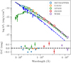 |
Fig. 1. Photometric SED of J22564–5910 obtained from literature photometry. The best-fitting model is shown with solid black line, with the contribution of the sdB shown with a blue-dashed line. The contribution of the IR excess, likely from a disc, is shown with a green-dashed line. The bottom shows the O–C between the observations and the best fitting model. |
The best fitting binary SED models using a Kurucz and black body model for the companion are given in Table 2. Both models are indicative of a rather cool sdB star combined with a cool component with a temperature between 5000 and 6000 K and a radius around 0.3 R⊙. The fitted reddening is higher than the value obtained from Lallement et al. (2019), but it has a large error. The model of the cool component is almost certainly non-physical, and the IR excess is likely caused by a disc-like structure, not a star. The reason for this is that such a star would require an unlikely combination of a high surface temperature with a very small radius. Secondly, if this would be a dwarf star or even an ultra-hot Jupiter (e.g. Lillo-Box et al. 2014), its spectral features should be visible in the spectra, which is not the case. It is clear that a more detailed model taking the possible geometry of the companion into account is necessary to adequately fit the SED. However, the temperature and radius of the sdB star are likely reliable, as they are supported by the presence of several strong He I lines and the absence of He II lines in the spectra.
Results of the SED fit.
3. Spectral analysis
The original EFOSC2 spectra were too low in resolution to show many features and only covered a small wavelength range. They did, however, show very broad H and He lines. If caused by stellar rotation alone, they would require a v sin i ∼ 1100 km s−1, which surpasses the critical velocity of sdBs. This discovery led to follow-up observations on 29-12-2018 using the Goodman spectrograph (Clemens et al. 2004) mounted on the 4.1-m Southern Astrophysical Research (SOAR) telescope on Cerro Pachón in Chile. Using a 930-line grating with a 0.45″ slit, the SOAR spectra have a better resolution and broader wavelength coverage but still had an insufficient signal-to-noise ratio (S/N). They did, however, show an indication of line splitting for the hydrogen lines and clear emission profiles for the Hα line, confirming the suspicion of gas or a magnetic field being present in the star. Based on these observations, follow-up observing proposals at both UVES and X-shooter were approved to study the unusual spectral features of J22564–5910.
In total, six extra spectra were obtained, including three UVES spectra and three X-shooter spectra. Two UVES spectra were taken one right after the other, followed by a third one, 1 month later. The X-shooter spectra have 1 week and 1 month in between them. These combinations allowed us to check for variability on different time scales. The X-shooter spectra were taken with a setup that favoured a higher S/N in the UVB and VIS in exchange for limited calibration of the NIR arm. Therefore the NIR spectra are of little use and are not included in our analysis. Details of these observations are given in Table 3.
Observing date, exposure time, signal-to-noise ratio (S/N), and resolution of the reduced spectra of the UVES and X-shooter observations of J22564–5910.
In Figs. A.1 and A.2, the normalised spectrum created by summing the three X-shooter spectra in both the UVB and VIS arm is shown. The spectrum shows several interesting features. Two Balmer lines, Hβ and Hγ, show a very clear triple absorption peak structure in their core. The same triple peak structure is visible in Hδ to Hη, but it is not as strong. The Hα line shows a very clear emission core that is stronger than the absorption part of the line. In the blue part of the spectrum, the calcium K line has a triple absorption peak structure with a very sharp absorption peak at the centre of the line. The centre absorption peak is interstellar in origin. The interstellar Ca-H line is visible near the centre of the Hη line. Furthermore, there are several He I lines visible. The He Iλ 4471 line shows the same triple peak structure visible in some of the hydrogen lines, but the centre of the line is shifted with respect to the rest wavelength by roughly 5 Å. The He I lines at 4921 and 5015 Å show an emission core and also appear shifted with respect to the rest wavelength. The He I line at 5875 Å also has a strong emission core, but it is roughly centred at its rest wavelength. At the end of the UVB arm of the spectrum, some bumps are visible which could be the Mg I triplet at 5167, 5173, and 5184 Å. However, the quality of the spectrum is not sufficient to confirm this. The two sharp absorption lines in the red part of the line are the Sodium doublet NaDλ 5890 and 5896 Å. Further in the red part of the spectrum, the O I triplet at 7774 Å shows core inversion similar to many of the He lines. The spectrum also shows some sharp lines in the red part, for example, at 6450−6520, 6960−7160, 7320−7400, and 7850−8100 Å. These lines are terrestrial and not related to the system.
3.1. Spectral trails
As multiple spectra are available, we can check if there is any change in the spectral features over time. In Fig. 2 the He I lines at 4471 and 5875 Å are shown together with Hα, Hβ, CaK, and the O Iλ 7774 line. The change in the Hα line is clearly visible. The emission core of the line varies between a single-peaked structure and a double-peaked structure. The He I 5875 shows a similar but much weaker change, an emission peak that shifts from a double peak or flat-topped structure to a sharper single peak. The CaK does not show clear variations. But the O Iλ 7774 line does show variations, with the strongest absorption peak moving from blue to red shifted and back. Interestingly, the latter two lines are typically not visible in sdB spectra as they require lower temperatures. These could be produced in circumstellar matter.
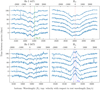 |
Fig. 2. Spectral trail of hydrogen and helium lines visible in the spectrum of J22564–5910. The rest wavelength of each line is shown in red dotted line. On the top left plot the Mg IIλ 4483 line is marked in green. On the bottom right plot the location of RK is indicated in blue dash-dotted line (see Sect. 6.1). The spectra are shown in order of observations – the time since the first spectrum is shown on the y axis. The bottom three spectra were taken with UVES, while the top three spectra were taken with X-shooter. The first two UVES spectra were taken back to back. The axes on the bottom of the plot shows wavelength, while that on the top shows velocity compared to the rest wavelength. |
The He Iλ 4471 line is a somewhat different feature. It can be interpreted as a triple absorption line that is shifted strongly from its central wavelength. Such a wavelength shift could be caused by the presence of a magnetic field (see Sect. 6.1). Another possible interpretation is that the line is a broad absorption line with an emission core centred on the rest wavelength of the line similar to the other two lines and that the rightmost absorption peak is caused by a different element (see Sect. 6.2).
The actual periodicity of the line changes cannot be determined from these spectra, but it is estimated to be of the order of several days to potentially even weeks. Another limiting factor of this analysis is that if the observed period is in fact due to rotation, the spectra should be affected by rotational smearing given the long exposure times (up to a third of the period). This implies that we might not be sampling the spectral variability completely. An important thing to notice is that the different lines vary with different periodicity. When comparing the Hα with the O Iλ 7774 line, at time 0, both are central peaked. At time 33 days, they have opposite absorption peaks with Hα being blue shifted and O I being red shifted. At time 75, they are both red shifted. This would indicate that they have different origins or originate in different locations in the disc.
3.2. Radial velocity variations
Given that the spectra are taken at different time intervals, it makes sense to attempt to check for radial velocity (RV) variations. However, this is complicated by the broad lines and varying line shapes. As the line cores of the hydrogen and helium lines vary strongly over time, they cannot be used to derive velocities. No clear, sharp lines are visible in the spectrum belonging to the system, so the only remaining approach is to use the wings of the hydrogen lines. Different approaches were attempted, using cross-correlation with a template spectrum and the best-observed spectra, as well as fitting Gaussian functions to the wings. The most successful approach was Gaussian fitting, as it resulted in the least difference between RVs determined for different lines in the same spectrum.
To derive the RVs, hydrogen lines from Hβ to Hη and H10 were used. For these lines, the line centres were removed. The wavelength region that is excluded was determined by eye by selecting the line part that varies the most in between the six spectra. Afterwards, a Gaussian was fitted to the wings of the same hydrogen line in all spectra, and the average value for its FWHM was used as a fixed value for the FWHM in the final fit. This way, all hydrogen lines were fitted, and the final RV is the average of the RV of the different hydrogen lines. The error was calculated as the standard deviation between the different lines.
The resulting RVs are shown in Fig. 3, and they are given in Table 3. As can be seen from that figure, almost all RVs are consistent with no significant RV variation. One spectrum, the first of the X-shooter spectra, shows a possible deviation. However, from these observations, it is not possible to conclude whether the system is RV variable or not.
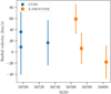 |
Fig. 3. Radial velocities of J22564–5910 as determined from the wings of the hydrogen lines. The first three measurements in blue are obtained from the UVES spectra, while the latter measurements are from the X-shooter spectra. Apart from one measurement, all RVs are consistent with no variation. |
4. TESS lightcurve
J22564–5910 (TIC 220490049) was observed by the Transiting Exoplanet Survey Satellite (TESS Ricker et al. 2015) during Sectors 01 and 28. Two-minute cadence data are not available because the object was not included in the TESS target list, but full-frame images (FFI) are available, with a 30-min cadence for Sector 01 and a 10-min cadence for Sector 28. We downloaded a cutout of 50 × 50 pixels using TESSCut (Brasseur et al. 2019) and performed photometry using the package lightkurve (Lightkurve Collaboration 2018). We used a 3 × 3 aperture centred on the star to avoid contamination by a bright (V = 9.79) star 2 arcmin away (which corresponds to only ∼6 pixels in TESS). The background was estimated using the same aperture in a region with no stars. Using the VARTOOLS program (Hartman & Bakos 2016), we performed a generalised Lomb-Scargle search (Zechmeister & Kürster 2009; Press et al. 1992) for periodic sinusoidal signals. In the periodogram (grey line in the top panel in Fig. 4), we find the strongest signal at P = 0.069764 ± 0.000005 d, with an associated false alarm probability of log(FAP) = − 152. The error on the period was estimated by running a differential evolution Markov chain Monte Carlo (DEMCMC) routine (Ter Braak 2006), employing the – nonlinfit command implemented in the VARTOOLS program. The phase-folded and phase-binned, TESS light curve is shown in red in the bottom panel of Fig. 4. The black line represents a fit of a harmonic series (Eq. (48) in Hartman & Bakos 2016, also used for the DEMCMC), to the phase-folded light curve. The peak-to-peak amplitude (defined as the difference of the maximum and minimum of the fit) of the phase-folded light curve is 23 mmag. We note, however, that due to the long exposure time (about one-tenth of the period), neither the amplitude nor the shape of this phase-folded light curve can be considered as reliable. After whitening the light curve for this signal, no other significant peaks remain in the periodogram (light blue line in the top panel in Fig. 4).
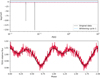 |
Fig. 4. Top: periodogram (grey) of the TESS light curve for J22564–5910. The light blue line is the re-calculated periodogram after the first whitening cycle. The red-dashed line indicates log(FAP) = − 4. Bottom: phase-folded (at the 0.069764 d period, respectively) and averaged (every 50 points) TESS light curve. |
The amplitude of the P = 0.069764 d peak is too high to be explained as a g-mode pulsation (Green et al. 2003), although the period is in the correct range. Most likely the variability is explained by a spot on the surface of the star, driven by the magnetic field, leading to periodic variations in observed flux as the star rotates. The uneven minima might suggest that two magnetic dark spots are present rather than one, which would be consistent with a dipole magnetic field (e.g. Jagelka et al. 2019). The non-sinusoidal shape of the phase-folded light curve (Fig. 4) is also typical of rotational modulation (e.g. Angus et al. 2018). Assuming the radius R = 0.1 R⊙ from the SED fit and rotational period of Prot = 0.069764 d, we derived a rotational velocity of Vrot = 73 km s−1.
5. Galactic orbit
Based on the Gaia EDR3 data, we can calculate the Galactic orbit of J22564–5910. For this the GALPY (Bovy 2015) python package was used. The parameters used as input for the Galpy code are shown in Table 4. They are all taken from Gaia EDR3, except the RV. For the RV, the weighted average of the RV measurements of the six spectra was taken. To calculate the errors, a Monte Carlo approach with 500 iterations was used. We find that J22564–5910 has a Galactic orbit with a maximum height above the plane (Zmax) of 688 ± 288 pc, a pericentre and apocentre distance (Rper, Rapo) of 3.7 ± 0.5 kpc and 7.7 ± 0.1 kpc, respectively, and an eccentricity (Ecc) of 0.36 ± 0.05 and an angular momentum of Jz = 1166 ± 88 kpc km s−1. These parameters are also summarised in Table 4.
Galactic orbit calculation of J22564–5910: input parameters for GALPY together with the resulting Galactic orbital parameters.
When comparing J22564–5910 to other hot subdwarf systems, from for example Luo et al. (2020), it would belong to the group of systems with relatively low Jz and above-average eccentricity (the average eccentricity in the sample of Luo is 0.23). It has similar kinematics as thick disc stars, but is located close to the boundary between the thick and thin disc (Pauli et al. 2006). While J22564–5910 lies on the edge of the Jz-eccentricity regions occupied by the hot subdwarfs in the thin and thick discs, it is certainly not an outlier relative to either of these two populations.
One can link the kinematic properties of a system to its age. Thin disc stars are initially born on planar and circular orbits. Over time, interactions with different Galactic components (spiral arms, the bar, and molecular clouds) make stellar orbits eccentric, induce radial migration, and drive the orbits off-plane. Therefore, the present-day eccentricity and vertical extent of the orbit of J22564–5910 may be linked to its age.
Asteroseismic observations combined with kinematics data show that stars typically found at Z-heights of about 500 pc, which approximates the time-averaged absolute Z-location of the system, have ages between 2 and 8 Gyr (Casagrande et al. 2016). Taking into account that the progenitors of sdB stars need to evolve off the MS, this would correspond to a progenitor’s primary masses of between 0.9 and 1.5 M⊙ (see, e.g. Vos et al. 2020). Furthermore, Frankel et al. (2018) show that stars can migrate in radial direction by 4 kpc on about an 8 Gyr timescale. Here the difference between Rper and Rapo of 4 kpc can be taken as a proxy for this migration process. The corresponding migration timescale of 8 Gyr is consistent with the age constraint based on the Z-location of the system. In summary, the Galactic orbit is consistent with an interaction of two older stars (for example, a He double WD merger), as well as a different formation channel involving an initial primary with a mass of up to about 1.5 M⊙.
In the Gaia images, a nearby star at nearly the same distance as J22564–5910 is visible. However, the two systems are likely not related. More information is given in Appendix B.
6. Interpretation
6.1. Magnetic fields
The triplet structure that is clearly visible in several hydrogen and helium lines immediately brings magnetic fields and Zeeman splitting to mind. This interpretation fits in with the expected evolution history of this system. As a single sdB formed by a merger, it is expected that J22564–5910 would acquire a strong magnetic field, generated through a dynamo process during the common-envelope evolution or the subsequent merger (e.g. Tout et al. 2008; García-Berro et al. 2012).
We applied a method similar to that of Kepler et al. (2013) to estimate the field strength necessary to produce the observed line splitting. The method relies on the fact that, for magnetic fields in the range 10 kG−2 MG, the observed line shift Δλ caused by a field B to the hydrogen lines can be approximated in the first order by
 (1)
(1)
where the wavelength is measured in Å and the magnetic field in MG. To account for contributions of higher-order terms, we utilised the models of Schimeczek & Wunner (2014) (see their Fig. 5) to estimate the averaged component separation predicted by the models. To calculate the observed separation for our obtained spectra, Gaussian lines were fitted to each Zeeman component. We only used the lines Hβ, Hγ, and Hδ; as for higher-order lines, the triplet structure is not apparent even for low fields (see, e.g. Fig. 5 of Kepler et al. 2013), and Hα is seen in emission. Moreover, we only applied this method to the spectra in which the three components could be identified for these lines. Depending on field structure and orientation, one or more components can be suppressed. Our method is illustrated in Fig. 5. For each spectrum, we searched for the field strength whose predicted separation could better explain the observed spectrum by minimising the difference between the observed and predicted separation for the three lines simultaneously. To estimate uncertainties, we drew flux values a thousand times, assuming a 10% uncertainty on the observed values, and we repeated the estimate for each of the simulated spectra. The results are shown in Table 5. Assuming that the field does not change significantly over time, which seems to be suggested by our consistent estimates, the average field is 656 ± 51 kG.
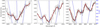 |
Fig. 5. Magnetic field estimate for the last obtained X-shooter spectrum. We note that Hδ, Hγ, and Hβ are shown from left to right. The observed spectrum is shown as a thin black line; a smoothed spectrum, restricted to the region where the Zeeman components were fitted, is shown as a thicker line. The fits to each Zeeman component are shown as red-dashed lines. The models of Schimeczek & Wunner (2014) are shown in grey, with the averaged separation including higher-order terms shown in blue, and the corresponding field strength shown on the right-hand side. The estimate for this spectrum was 660 ± 62 kG. |
Field estimates for the three spectra in which three Zeeman components can be identified for the Hβ, Hγ, and Hδ lines.
Emission in Hα is not an atypical phenomenon amongst magnetic stars. Magnetically active (sub-)giants, for example, show chromospheric emission lines in Hα, but at the same time also in the cores of the Ca II H and K lines, as well as sometimes other lines in the optical or ultraviolet (Wilson 1963, 1968; Gray & Corbally 2009). For some of these stars, time-variability in the chromospheric Hα emission, which is not correlated to the rotation period, has also been reported, though, the exact origin of the variability is not yet understood (e.g., Dorren et al. 1984; Vida et al. 2015; Kővári et al. 2019; Werner et al. 2020).
There is also a small group of three cool (effective temperatures between 7500 K and 7865 K), magnetic and apparently single WDs known that exhibit Zeeman-split Balmer emission lines (Greenstein & McCarthy 1985; Reding et al. 2020; Gänsicke et al. 2020). It is thought that a conductive planet in a close orbit around these stars could result in the generation of electric currents that heat the regions near the magnetic poles of the WD. The planet, in this case, would have formed in a metal-rich debris disc that was left over by a double WD merger that could have produced the magnetic WD (Li et al. 1998; Wickramasinghe et al. 2010). However, in contrast to our star, the emission lines in these WDs are not only seen in Hα but also Hβ and they are triple-peaked instead of single or double-peaked.
Last but not least, for magnetic O- and B-type main sequence stars that host a wind-fed, co-rotating, circumstellar magnetosphere, emission in Hα is the primary visible magnetospheric diagnostic. In Fig. 6, we show such a model applied to our system. In slowly rotating stars, the material persists within the magnetosphere only over the free-fall timescale, and it is pulled back onto the star by gravity (so-call dynamical magnetosphere, Landstreet & Borra 1978; Ud-Doula & Owocki 2002; Petit et al. 2013). However, if the star is rapidly rotating or if the magnetic field strength is high enough, the co-rotating material in the magnetosphere can reach high enough rotational velocities so that the gravitational infall can be prevented. This is the case when the Alfvén radius RA, which characterises the maximum height of closed magnetic loops, exceeds the Keplerian co-rotation radius, RK (point of balance between gravitational and centrifugal force). While below RK, the star retains a dynamical magnetosphere, above RK and extending to RA, a so-called centrifugal magnetosphere forms. Herein, the trapped wind material accumulates into a relatively dense, stable, and long-lived ‘rigidly rotating magnetosphere’ (RRM, Townsend & Owocki 2005; Townsend et al. 2007). According to the RRM model, the distribution of the material then depends on the tilt, β, of the magnetic axis with respect to the rotational axis of the star. While for β = 0°, a continuous torus in the magnetic equatorial plane forms, two distinct plasma clouds are expected near the intersections of the magnetic and rotational equatorial planes for β = 90°. The typical RRM geometry, thus, produces a double-humped emission profile, when the circumstellar magnetosphere is seen face on. Since the magnetosphere has its highest density close to RK, the Hα emission is also found to peak close to RK (typically around 1.25 × RK, Shultz et al. 2020). The remaining shape of the Hα emission then depends on the geometry of the RRM. Non-eclipsing stars with small β show emission at all velocities across the line profile, whereas non-eclipsing stars with large β display emission only outside of ±RK at maximum emission. The emission line profile is modulated by the rotation of the object. As the projected distance of the clouds from the star decreases, and – at the same time – the projected area of the clouds becomes smaller when changing from face-on to edge-on, the Hα emission bumps decrease in strength (Shultz et al. 2020).
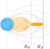 |
Fig. 6. Illustration for the structure of the system for the magnetic interpretation. The spinning subdwarf (in blue) generates a dipolar magnetic field around it, which is not necessarily aligned with the spin. The wind material in the innermost region, within Kepler radius RK, has no centrifugal support and can fall freely back onto the star, thus forming a dynamical magnetosphere. The material between the Keplerian co-rotation radius RK and the Alfvén radius RA has centrifugal support. It cannot fall back onto the star, thus forming a much denser rigidly rotating magnetosphere. The illustration is inspired by Petit et al. (2013). |
Since, also in our star, we detect this time-variable, double-humped Hα emission profile, the RRM model appears attractive. The multi-component absorption features seen for the CaII and OI originating in the circumstellar material (Fig. 7) could also be explained by the distribution of the material in the magnetosphere. Magneto-hydrodynamic simulation studies (e.g., Ud-Doula & Owocki 2002; Ud-Doula et al. 2008) show that in case of a large-scale, dipole magnetic field, a magnetosphere forms when the wind magnetic confinement parameter (η⋆) is larger than one:
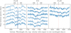 |
Fig. 7. Same as Fig. 2, but spectral trail of lines likely to originate in the circumstellar material visible in the spectrum of J22564–5910. For the Ca II line, the UVES spectra show only noise and they are not shown here. The other two components of the Ca IR triplet are not visible in the spectra. |
Here Beq = Bd/2 is the field strength at the magnetic equatorial surface radius, R⋆, and ṀB = 0 and v∞ are the fiducial mass-loss rate and terminal wind speed that the star would have in the absence of any magnetic field (all in centimeter-gram-second units). Assuming a typical mass loss rate for an sdB star of 10−11.5 M⊙ yr−1 (Vink & Cassisi 2002), v∞ = vesc = 1338 km s−1 (assuming M = 0.47 M⊙, and R = 0.1 R⊙, Hamann et al. 1981; Howarth 1987) and R = 0.1 R⊙; we find that in case of J22564–5910, a magnetosphere can already form for Beq ⪆ 24 G. This is many orders of magnitude below what we find above, thus, the requirement for a centrifugal magnetosphere (RA > RK) can be easily fulfilled. Assuming M = 0.47 M⊙, and R = 0.1 R⊙, we find RK = 5.5 R⋆ assuming the 0.07 d period observed in the TESS light curve is the rotational period of the star. The Alfvén radius, RA, can be estimated from the wind magnetic confinement parameter, η*, via RA/R⋆ ≈ 0.3 (η* + 0.4)1/4 (Ud-Doula et al. 2008). Here, we find RA = 118.6 R⋆, but it should be noted that the exact value depends on the mass loss rate and terminal wind velocity, which we can only estimate. Moreover, additional circumstellar material might be present as a result of the possible merger, which we do not take into account here. What can, however, be taken away from this is that a centrifugal magnetosphere can be expected2.
Since the rigid-body rotation of the circumstellar magnetosphere implies that the line of sight velocity, v, is directly proportional to the projected distance from the star (v/(vrot sin i) = r/R⋆), one can in principle test the circumstellar magnetosphere scenario with the Hα line profile directly (Shultz et al. 2020), as the emission peaks should occur around RK (see above). We find that the observed emission peaks of the Hα line in J22564–5910 would be located at RK if we assume for the 0.07 d period an inclination angle of i ≈ 20° (blue dashed-dotted lines in Fig. 2). Unfortunately, due to the lack of any photospheric metal lines and the high magnetic field, it is not possible to measure vrot sin i, plus the lack of knowledge on stellar mass adds another uncertainty when calculating RK. In addition, we note that if the 0.07 d period is indeed the rotational period, then the spectra should suffer considerably from rotational smearing due to the long exposure time (one quarter of the period). Hence the line profile shapes may not be considered as reliable. Thus, based on the current data, it is not possible to entirely confirm the RRM model.
6.2. Circumstellar material (non-magnetic scenario)
Complicated spectral line profiles may also have another explanation that does not require magnetic fields. In this section, we investigate the idea that the spectral lines are shaped by circumstellar material (CM). Such material is often present in interacting binaries or hot stars and might be present in our system too. It gives rise to emission lines of a rather complicated shape which may be superposed on the absorption lines originating from the stellar atmosphere. The result would be even more complicated spectral line profiles. In this scenario, double absorption such as in the Hα line would not be composed of two absorption lines but from a single broad absorption line (from the stellar atmosphere) filled up by more narrow central emission from the CM. Lines with triple absorption could be understood as a single broad absorption from the photosphere filled in by a double peak emission from CM.
The most natural form of circumstellar material in a binary system or in a merger of two stars is probably an accretion disc. Typically, such a disc gives rise to a double-peaked emission (unless seen pole-on). Thus an inclined disc might explain triple absorption profile seen best in Hβ. To demonstrate the idea that such line profiles may be due to CM, we performed a synthetic spectra calculation. As this analysis aims to be a qualitative one and not a quantitative fit to the spectra, we used a master spectrum for the comparison of the models with the observations. This master spectrum was obtained by summing all three X-shooter spectra without any RV corrections for stellar motion. The spectra were then normalised.
As a first step, we calculated the stellar atmosphere model using the TLUSTY code (Hubeny & Lanz 1995). These are 1D non-local-thermodynamic-equilibrium (NLTE) atmosphere models. The spectra emerging from these atmosphere models were calculated using the code SYNSPEC (Hubeny & Lanz 2017). We assumed Teff = 26 000 K, log g = 6.1 [cgs], and solar chemical composition. Such synthetic spectra of the Hβ line are shown in Fig. 8. One can see very strong, deep, and relatively sharp absorption originating from the stellar atmosphere. The major challenge of this model is filling this profile with emission. This intrinsic spectrum of the star was used as a boundary condition to calculate the spectra of the star and CM, for which we used the SHELLSPEC code (Budaj & Richards 2004). It is designed to calculate light curves and spectra of interacting binaries embedded in a 3D moving CM, assuming local thermodynamic equilibrium (LTE) and optically thin scattering. The assumed stellar mass, radius, and projected equatorial rotation velocity are M = 0.47 M⊙, R = 0.1 R⊙, and v sin i = 70 km s−1, respectively. Quadratic limb darkening coefficients for the star from Claret (2000) were assumed. The chemical composition of the CM was identical to that of the star. CM had the form of an accretion disc. Synthetic spectra of the most interesting and most complicated Hβ line are also shown in Fig. 8. One can clearly see a double peak emission from the disc filling in the central part of the absorption from the photosphere. The result might look like a triple absorption.
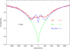 |
Fig. 8. Synthetic spectra of the Hβ line compared with the observations. The theoretical spectrum of the star without the disc is shown in green. The theoretical spectrum of the star + disc is shown in blue. The observed spectrum is shown in red. More details may be found in Sect. 6.2. |
The properties of the CM are described below. The disc was modelled using an object called NEBULA in the SHELLSPEC code. It is a flared disc characterised by its inner, Rin, and outer, Rout, radius, and an inclination i. Its density is decreasing in the radial direction as a power law, ρ(r) = ρin(r/rin)ρexp, and in the vertical direction as a Gaussian. It is characterised by the density at the inner radius ρin and exponent ρexp. We assumed ρexp = −1 based on Budaj et al. (2005). The temperature, similarly, has a radial power-law dependence characterised by Tin and exponent Texp. The velocity field is Keplerian. In reality, it may be much more complicated. The disc may have a radial inflow component and is also often accompanied by winds, jets, or other outflows. That is why we also introduced a simple parameter called ‘turbulence’, vT. Electron number densities were calculated from the density, temperature, and chemical composition assuming LTE. Values of all these parameters are summarised in Table 6.
Properties of the circumstellar medium (CM) used in the SHELLSPEC model.
We can conclude that CM material might explain the complicated shapes of the spectral lines we observe in this star. However, these calculations should be understood only as a demonstration of the effect, and disc parameters (mainly densities) represent rather a lower limit. In reality, the geometry, velocity field, and behaviour of state quantities of the CM may be much more complicated than our simple disc model. Their effect will be mainly to smooth the ideal theoretical line profile. We experimented with dozens of other models of CM-like shells, discs, and temperature inversions, and many of them produce a similar outcome, that is to say triple absorption profiles. The most difficult problem is to fill in the sharp central absorption peak.
The advantage of this model is that it also has the potential to explain the IR excess observed in the SED, as well as the emission seen in other H and He lines in the spectra. The change in the line profiles that is shown in Fig. 2 might be explained by the disc model as well. Accretion structures are not necessarily stable and can change over time, causing changes in the line profiles. If a magnetic field is present, this can also affect the structure and cause variability. Furthermore, if there would be a secondary body present in the system, it can cause precession of the disc which would cause changes in the emission cores of the H and He lines. This body would have to be much closer than the nearby companion described in Appendix B.
6.3. CE outcome versus merger
The three formation channels for hot subdwarf stars are stable RLOF, CE ejection, and a merger. Based on the observations, we can exclude two of these channels with a very high likelihood.
All known wide sdB binaries that formed through the stable RLOF channel have FGK type companions (e.g. Vos et al. 2017). These companions can be clearly seen in high-resolution spectroscopy. There is no sign of such a companion in J22564–5910, and thus this scenario can be excluded. There are then two possibilities left. J22564–5910 can be a close binary with a dM or WD companion, or it can be a single merger product.
In the case that J22564–5910 would be an sdB+dM binary, we can compare it to the known population of sdB+dM binaries. These systems all have short orbits, with their period distribution peaking at less than a day. Using the LCURVE package (Copperwheat et al. 2010, Appendix A), we computed the expected amplitude for the reflection effect in sdB+dM binaries for a typical dM companion at different orbital periods and inclinations angles (see Fig. 9). From this figure, it is clear that such a binary would be detected in the TESS light curve for orbital periods up to ∼8 days. Since these systems are nearly never found at orbital periods larger than a few days, we can conclude that the sdB+dM possibility is very unlikely.
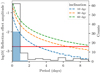 |
Fig. 9. Expected reflection effect for a typical dM companion at different inclination angles as a function of orbital period. The solid red line shows the detection limit of TESS. On the right axis, the known period distribution of sdB+dM binaries is shown in blue. In black, the period distribution of sdB binaries with an unknown companion (low mass MS or WD) is shown. The period distributions were taken from Kupfer et al. (2015). |
The above considerations leave the sdB+WD possibility. Such systems do not show a significant reflection effect in the light curves, but they can show ellipsoidal modulations. LCURVE models show that such effects would be detectable for typical WD companions for orbital periods up to ∼0.3 days. As sdB+WD binaries are observed on longer orbital periods than that, the light curve alone is not sufficient to exclude this possibility.
To further judge the sdB+WD option, the RVs derived from the spectra can be used. Known sdB+WD systems have short orbital periods and thus high RV variations. The RVs that are derived in Sect. 3.2 show possible variations of up to ∼30 km s−1. This would correspond to sdB+WD systems on orbital period > 5 days, which is very exceptional for sdB+WD systems (Kupfer et al. 2015; Prince et al. 2019). The RV analysis used the wings of the H lines, which originate from the central star, and they are likely not significantly influenced by the disc.
Based on the limits obtained from the light curve and the spectra, we can with high certainty say that J22564–5910 is a single sdB and thus a merger product. The derived properties suggest that the object is in a core-He burning phase. For typical double-degenerate mergers, this phase is only reached long after the merger (∼106 yr), at which point all the circumstellar material resulting from the merger should have been lost. Additionally, He-core burning products of double degenerate mergers are expected to show higher temperatures and be H-deficient, which is not the case here (Dan et al. 2014; Schwab 2018). Therefore, a WD+MS merger is a more likely scenario for the formation of J22564–5910 as in this case the He-core burning phase can occur at lower effective temperature, and high amounts of hydrogen are still expected (Zhang et al. 2017).
In the case that J22564–5910 would indeed be a magnetic system, there is an extra argument to be made against the CE formalism. While the dynamo actions arising during the CE phase can indeed cause magnetic fields, models show that these fields are weak and do not last long after the CE ejection (see e.g. Potter & Tout 2010).
7. Discussion and conclusions
J22564–5910 is a hot subdwarf star with very shallow, variable, multi-peaked H and He lines, with an Hα emission, IR excess, photometric variability, and possibly with a high rotational velocity. Based on the multi-band photometry, time-resolved spectroscopy, Gaia astrometry, and the TESS light curve, we have found two possible interpretations of the spectrum. The first one is that the multi-peaked spectral features are caused by the existence of a magnetic field of about 650 kG. The IR excess in the SED and the emission core in the Hα line can then be caused by the formation of a magnetosphere. Similarly, this would explain the time variation of the spectral lines. A second possibility is the existence of a circumstellar disc that would explain both the IR excess and the special line shapes. Changes in the line shapes can be explained by variations in the circumstellar material or a precessing disc.
The major problem with this star is that the observed hydrogen lines are too shallow. Helium lines are equally shallow and broad compared with theoretically expected lines originating from the stellar photosphere. Some other hot subdwarf stars show a relatively narrow emission in Hα. This, however, happens at much hotter temperatures and is caused by NLTE effects that affect the level populations of the hydrogen atom (e.g. Rauch et al. 2010; Reindl et al. 2014; Latour et al. 2015; Dorsch et al. 2020). Thus we can exclude that this is the reason for the observed emission in Hα and shallowness of other H and He lines.
All hot subdwarf stars are formed through a binary interaction, whether it is a stable RLOF, a CE ejection phase, or a merger. In this case, the observations point strongly to a post-merger single sdB. A CE ejection resulting in a close binary with a WD companion is possible but very unlikely. The presence of circumstellar material in the system and the line variations would indicate that we are observing this system very closely after the interaction phase. Both of our interpretations of the observations are consistent with the merger scenario, as a magnetic field could be instilled in the final product, and a significant amount of mass would end up around the sdB.
Regardless of whether the observed features are caused by magnetism or circumstellar matter, J22564–5910 is a very interesting system that could provide insight in the early dawn after a binary merger phase. It has the potential to solve several outstanding problems in the physical explanation of this phase, including the discrepancy between the predicted high rotational velocities for post merger products versus the observed low rotation rates of single sdBs, or the predictions that mergers can instill magnetic fields in their products. If J22564–5910 turns out to be a a magnetic sdB, then it could be a long sought immediate ancestor of strongly magnetic WDs. This could provide vital clues to help understand the magnetic field evolution across the Hertzsprung Russell diagram.
The likely origin of J22564–5910 is the CE evolution of an RGB and a He-WD. The CE episode would either have led to a merger within the red giant envelope, between the He-RG core and the He-WD, or to a short-period He-WD binary which later merges due to gravitational wave emission (Han et al. 2002). In this case, the observed properties of J22564–5910 may be explained by it being a particularly young member of the class of single sdBs.
The two interpretations offered here are not mutually exclusive and are not the only possible explanations of this system, although in our opinion they are the most likely. It is perfectly possible that both a circumstellar disc and a magnetic field are present in the system. The spectrum of this system contains multiple components which, with the currently available observations, are impossible to disentangle. Further investigation of, for example, spectropolarimetry can confirm if a magnetic field is really present in the system. Time-resolved spectroscopy will allow for the investigation of the line profile variations. Observations in the UV or even in the X-ray domain with eRosita would be valuable to constrain models of the system as, for example, X-ray flares may be expected (e.g. Groote & Schmitt 2004). On the other end of the spectrum, observations in the far-IR with, for example, ALMA would provide clues as to structure of the gas and the dust present in the system.
Observationally, centrifugal magnetospheres are detected in stars with log(RA/RK) > 0.7 (Shultz et al. 2020).
Acknowledgments
The authors would like to thank Uli Heber for his very helpful referee report. This work was supported by a fellowship for postdoctoral researchers from the Alexander von Humboldt Foundation awarded to JV. IP was partially funded by the Deutsche Forschungsgemeinschaft under grant GE2506/12-1. J.B. was supported by the VEGA 2/0031/18 and by the Slovak Research and Development Agency under the contract No. APVV-20-0148. V.S. is supported by the Deutsche Forschungsgemeinschaft (DFG) through grant GE 2506/9-1 M.U. acknowledges financial support from CONICYT Doctorado Nacional in the form of grant number No: 21190886 and the ESO studentship program. Based on observations collected at the European Southern Observatory under ESO programmes 0101.D-0440, 0103.D-0129 and 0104.D-0596. Based in part on observations obtained at the SOAR telescope, which is a joint project of the Ministério da Ciência, Tecnologia e Inovações (MCTI/LNA) do Brasil, the US National Science Foundation’s NOIRLab, the University of North Carolina at Chapel Hill (UNC), and Michigan State University (MSU). This work has made use of data from the European Space Agency (ESA) mission Gaia (https://www.cosmos.esa.int/gaia), processed by the Gaia Data Processing and Analysis Consortium (DPAC, https://www.cosmos.esa.int/web/gaia/dpac/consortium). Funding for the DPAC has been provided by national institutions, in particular the institutions participating in the Gaia Multilateral Agreement. This research made use of Astropy, a community-developed core Python package for Astronomy (Astropy Collaboration 2013).
References
- Angus, R., Morton, T., Aigrain, S., Foreman-Mackey, D., & Rajpaul, V. 2018, MNRAS, 474, 2094 [Google Scholar]
- Astropy Collaboration (Robitaille, T. P., et al.) 2013, A&A, 558, A33 [NASA ADS] [CrossRef] [EDP Sciences] [Google Scholar]
- Belokurov, V., Penoyre, Z., Oh, S., et al. 2020, MNRAS, 496, 1922 [Google Scholar]
- Bovy, J. 2015, ApJS, 216, 29 [NASA ADS] [CrossRef] [Google Scholar]
- Brasseur, C. E., Phillip, C., Fleming, S. W., Mullally, S. E., & White, R. L. 2019, Astrophysics Source Code Library [record ascl:1905.007] [Google Scholar]
- Budaj, J., & Richards, M. T. 2004, Contrib. Astron. Obs. Skaln. Pleso, 34, 167 [NASA ADS] [Google Scholar]
- Budaj, J., Richards, M. T., & Miller, B. 2005, ApJ, 623, 411 [NASA ADS] [CrossRef] [Google Scholar]
- Casagrande, L., Silva Aguirre, V., Schlesinger, K. J., et al. 2016, MNRAS, 455, 987 [Google Scholar]
- Claret, A. 2000, A&A, 363, 1081 [NASA ADS] [Google Scholar]
- Clemens, J. C., Crain, J. A., & Anderson, R. 2004, in Ground-based Instrumentation for Astronomy, eds. A. F. M. Moorwood, & M. Iye, SPIE Conf. Ser., 5492, 331 [NASA ADS] [CrossRef] [Google Scholar]
- Copperwheat, C. M., Marsh, T. R., Dhillon, V. S., et al. 2010, MNRAS, 402, 1824 [Google Scholar]
- Dan, M., Rosswog, S., Brüggen, M., & Podsiadlowski, P. 2014, MNRAS, 438, 14 [NASA ADS] [CrossRef] [Google Scholar]
- Dorren, J. D., Guinan, E. F., & McCook, G. P. 1984, PASP, 96, 250 [CrossRef] [Google Scholar]
- Dorsch, M., Latour, M., Heber, U., et al. 2020, A&A, 643, A22 [EDP Sciences] [Google Scholar]
- Elkin, V. G. 1996, A&A, 312, L5 [NASA ADS] [Google Scholar]
- Ferrario, L., de Martino, D., & Gänsicke, B. T. 2015, Space Sci. Rev., 191, 111 [Google Scholar]
- Frankel, N., Rix, H.-W., Ting, Y.-S., Ness, M., & Hogg, D. W. 2018, ApJ, 865, 96 [NASA ADS] [CrossRef] [Google Scholar]
- Gaia Collaboration (Brown, A. G. A., et al.) 2021, A&A, 650, C3 [EDP Sciences] [Google Scholar]
- Gänsicke, B. T., Rodríguez-Gil, P., Gentile Fusillo, N. P., et al. 2020, MNRAS, 499, 2564 [CrossRef] [Google Scholar]
- García-Berro, E., Lorén-Aguilar, P., Aznar-Siguán, G., et al. 2012, ApJ, 749, 25 [CrossRef] [Google Scholar]
- Gray, R. O., & Corbally, C. J. 2009, Stellar Spectral Classification (Princeton: Princeton University Press) [Google Scholar]
- Green, E. M., Fontaine, G., Reed, M. D., et al. 2003, ApJ, 583, L31 [Google Scholar]
- Greenstein, J. L., & McCarthy, J. K. 1985, ApJ, 289, 732 [CrossRef] [Google Scholar]
- Groote, D., & Schmitt, J. H. M. M. 2004, A&A, 418, 235 [NASA ADS] [CrossRef] [EDP Sciences] [Google Scholar]
- Hall, P. D., & Jeffery, C. S. 2016, MNRAS, 463, 2756 [NASA ADS] [CrossRef] [Google Scholar]
- Hamann, W. R., Gruschinske, J., Kudritzki, R. P., & Simon, K. P. 1981, A&A, 104, 249 [NASA ADS] [Google Scholar]
- Han, Z., Podsiadlowski, P., Maxted, P. F. L., Marsh, T. R., & Ivanova, N. 2002, MNRAS, 336, 449 [Google Scholar]
- Han, Z., Podsiadlowski, P., Maxted, P. F. L., & Marsh, T. R. 2003, MNRAS, 341, 669 [NASA ADS] [CrossRef] [Google Scholar]
- Hartman, J. D., & Bakos, G. Á. 2016, Astron. Comput., 17, 1 [Google Scholar]
- Heber, U. 2016, PASP, 128, 082001 [Google Scholar]
- Heber, U., Geier, S., & Gaensicke, B. 2013, Eur. Phys. J. Web Conf., 43, 04002 [NASA ADS] [CrossRef] [EDP Sciences] [Google Scholar]
- Henden, A. A., Levine, S., Terrell, D., & Welch, D. L. 2015, Am. Astron. Soc. Meet. Abstr., 225, 336.16 [Google Scholar]
- Howarth, I. D. 1987, MNRAS, 225, 33P [Google Scholar]
- Hubeny, I., & Lanz, T. 1995, ApJ, 439, 875 [Google Scholar]
- Hubeny, I., & Lanz, T. 2017, ArXiv e-prints [arXiv:1706.01859] [Google Scholar]
- Iben, I., Jr. 1990, ApJ, 353, 215 [NASA ADS] [CrossRef] [Google Scholar]
- Iben, I., Jr., & Tutukov, A. V. 1986, ApJ, 311, 742 [NASA ADS] [CrossRef] [Google Scholar]
- Igoshev, A. P., Perets, H. B., & Michaely, E. 2020, MNRAS, 494, 1448 [NASA ADS] [CrossRef] [Google Scholar]
- Jagelka, M., Mikulášek, Z., Hümmerich, S., & Paunzen, E. 2019, A&A, 622, A199 [NASA ADS] [CrossRef] [EDP Sciences] [Google Scholar]
- Jordan, S., Werner, K., & O’Toole, S. J. 2005, A&A, 432, 273 [NASA ADS] [CrossRef] [EDP Sciences] [Google Scholar]
- Jordan, S., Bagnulo, S., Werner, K., & O’Toole, S. J. 2012, A&A, 542, A64 [NASA ADS] [CrossRef] [EDP Sciences] [Google Scholar]
- Kepler, S. O., Pelisoli, I., Jordan, S., et al. 2013, MNRAS, 429, 2934 [Google Scholar]
- Kővári, Z., Strassmeier, K. G., Oláh, K., et al. 2019, A&A, 624, A83 [NASA ADS] [CrossRef] [EDP Sciences] [Google Scholar]
- Kupfer, T., Geier, S., Heber, U., et al. 2015, A&A, 576, A44 [NASA ADS] [CrossRef] [EDP Sciences] [Google Scholar]
- Kurucz, R. L. 1979, ApJS, 40, 1 [NASA ADS] [CrossRef] [Google Scholar]
- Lallement, R., Babusiaux, C., Vergely, J. L., et al. 2019, A&A, 625, A135 [NASA ADS] [CrossRef] [EDP Sciences] [Google Scholar]
- Landstreet, J. D. 2004, in The A-Star Puzzle, eds. J. Zverko, J. Ziznovsky, S. J. Adelman, & W. W. Weiss, 224, 423 [NASA ADS] [Google Scholar]
- Landstreet, J. D., & Borra, E. F. 1978, ApJ, 224, L5 [NASA ADS] [CrossRef] [Google Scholar]
- Landstreet, J. D., Bagnulo, S., Fossati, L., Jordan, S., & O’Toole, S. J. 2012, A&A, 541, A100 [NASA ADS] [CrossRef] [EDP Sciences] [Google Scholar]
- Latour, M., Fontaine, G., Green, E. M., & Brassard, P. 2015, A&A, 579, A39 [NASA ADS] [CrossRef] [EDP Sciences] [Google Scholar]
- Leone, F., Corradi, R. L. M., Martínez González, M. J., Asensio Ramos, A., & Manso Sainz, R. 2014, A&A, 563, A43 [NASA ADS] [CrossRef] [EDP Sciences] [Google Scholar]
- Li, J., Ferrario, L., & Wickramasinghe, D. 1998, ApJ, 503, L151 [NASA ADS] [CrossRef] [Google Scholar]
- Lightkurve Collaboration (Cardoso, J. V. D. M., et al.) 2018, Astrophysics Source Code Library [record ascl:1812.013] [Google Scholar]
- Lillo-Box, J., Barrado, D., Moya, A., et al. 2014, A&A, 562, A109 [NASA ADS] [CrossRef] [EDP Sciences] [Google Scholar]
- Lindegren, L., Klioner, S. A., Hernández, J., et al. 2021a, A&A, 649, A2 [EDP Sciences] [Google Scholar]
- Lindegren, L., Bastian, U., Biermann, M., et al. 2021b, A&A, 649, A4 [EDP Sciences] [Google Scholar]
- Luo, Y., Németh, P., & Li, Q. 2020, ApJ, 898, 64 [Google Scholar]
- Mardling, R., & Aarseth, S. 1999, in The Dynamics of Small Bodies in the Solar System, A Major Key to Solar System Studies, eds. B. A. Steves & A. E. Roy, NATO Adv. Study Inst. (ASI) Ser. C, 522, 385 [NASA ADS] [CrossRef] [Google Scholar]
- Mathys, G., Hubrig, S., Mason, E., et al. 2012, Astron. Nachr., 333, 30 [Google Scholar]
- Momany, Y., Zaggia, S., Montalto, M., et al. 2020, Nat. Astron., 4, 1092 [Google Scholar]
- Neiner, C., Mathis, S., Alecian, E., et al. 2015, in Polarimetry, eds. K. N. Nagendra, S. Bagnulo, R. Centeno, & M. Jesús Martínez González, 305, 61 [Google Scholar]
- O’Toole, S. J., Jordan, S., Friedrich, S., & Heber, U. 2005, A&A, 437, 227 [CrossRef] [EDP Sciences] [Google Scholar]
- Pauli, E. M., Napiwotzki, R., Heber, U., Altmann, M., & Odenkirchen, M. 2006, A&A, 447, 173 [NASA ADS] [CrossRef] [EDP Sciences] [Google Scholar]
- Pelisoli, I., Vos, J., Geier, S., Schaffenroth, V., & Baran, A. S. 2020, A&A, 642, A180 [NASA ADS] [CrossRef] [EDP Sciences] [Google Scholar]
- Petit, V., Owocki, S. P., Wade, G. A., et al. 2013, MNRAS, 429, 398 [NASA ADS] [CrossRef] [Google Scholar]
- Potter, A. T., & Tout, C. A. 2010, MNRAS, 402, 1072 [NASA ADS] [CrossRef] [Google Scholar]
- Press, W. H., Teukolsky, S. A., Vetterling, W. T., & Flannery, B. P. 1992, Numerical Recipes in C. The Art of Scientific Computing (Cambridge: Cambridge University Press) [Google Scholar]
- Prince, T., Burdge, K., Bellm, E., et al. 2019, Am. Astron. Soc. Meet. Abstr., 233, 418.05 [NASA ADS] [Google Scholar]
- Rauch, T., Werner, K., & Kruk, J. W. 2010, Ap&SS, 329, 133 [NASA ADS] [CrossRef] [Google Scholar]
- Reding, J. S., Hermes, J. J., Vanderbosch, Z., et al. 2020, ApJ, 894, 19 [NASA ADS] [CrossRef] [Google Scholar]
- Reindl, N., Rauch, T., Werner, K., Kruk, J. W., & Todt, H. 2014, A&A, 566, A116 [NASA ADS] [CrossRef] [EDP Sciences] [Google Scholar]
- Ricker, G. R., Winn, J. N., Vanderspek, R., et al. 2015, J. Astron. Telesc. Instrum. Syst., 1, 014003 [Google Scholar]
- Riello, M., De Angeli, F., Evans, D. W., et al. 2021, A&A, 649, A3 [NASA ADS] [CrossRef] [EDP Sciences] [Google Scholar]
- Sabin, L., Hull, C. L. H., Plambeck, R. L., et al. 2015, MNRAS, 449, 2368 [NASA ADS] [CrossRef] [Google Scholar]
- Saio, H., & Jeffery, C. S. 2000, MNRAS, 313, 671 [NASA ADS] [CrossRef] [Google Scholar]
- Schimeczek, C., & Wunner, G. 2014, ApJS, 212, 26 [CrossRef] [Google Scholar]
- Schlafly, E. F., Meisner, A. M., & Green, G. M. 2019, ApJS, 240, 30 [Google Scholar]
- Schneider, F. R. N., Ohlmann, S. T., Podsiadlowski, P., et al. 2019, Nature, 574, 211 [Google Scholar]
- Schwab, J. 2018, MNRAS, 476, 5303 [Google Scholar]
- Shultz, M. E., Owocki, S., Rivinius, T., et al. 2020, MNRAS, 499, 5379 [NASA ADS] [CrossRef] [Google Scholar]
- Skrutskie, M. F., Cutri, R. M., Stiening, R., et al. 2006, AJ, 131, 1163 [NASA ADS] [CrossRef] [Google Scholar]
- Ter Braak, C. J. F. 2006, Stat. Comput., 16, 239 [Google Scholar]
- Toonen, S., Hamers, A., & Portegies Zwart, S. 2016, Comput. Astrophys. Cosmol., 3, 6 [NASA ADS] [CrossRef] [Google Scholar]
- Toonen, S., Portegies Zwart, S., Hamers, A. S., & Bandopadhyay, D. 2020, A&A, 640, A16 [NASA ADS] [CrossRef] [EDP Sciences] [Google Scholar]
- Tout, C. A., Wickramasinghe, D. T., Liebert, J., Ferrario, L., & Pringle, J. E. 2008, MNRAS, 387, 897 [NASA ADS] [CrossRef] [Google Scholar]
- Townsend, R. H. D., & Owocki, S. P. 2005, MNRAS, 357, 251 [NASA ADS] [CrossRef] [Google Scholar]
- Townsend, R. H. D., Owocki, S. P., & Ud-Doula, A. 2007, MNRAS, 382, 139 [NASA ADS] [CrossRef] [Google Scholar]
- Ud-Doula, A., & Owocki, S. P. 2002, ApJ, 576, 413 [NASA ADS] [CrossRef] [Google Scholar]
- Ud-Doula, A., Owocki, S. P., & Townsend, R. H. D. 2008, MNRAS, 385, 97 [NASA ADS] [CrossRef] [Google Scholar]
- Vida, K., Korhonen, H., Ilyin, I. V., et al. 2015, A&A, 580, A64 [NASA ADS] [CrossRef] [EDP Sciences] [Google Scholar]
- Vink, J. S., & Cassisi, S. 2002, A&A, 392, 553 [NASA ADS] [CrossRef] [EDP Sciences] [Google Scholar]
- Vos, J., Østensen, R. H., Degroote, P., et al. 2012, A&A, 548, A6 [NASA ADS] [CrossRef] [EDP Sciences] [Google Scholar]
- Vos, J., Østensen, R. H., Németh, P., et al. 2013, A&A, 559, A54 [NASA ADS] [CrossRef] [EDP Sciences] [Google Scholar]
- Vos, J., Østensen, R. H., Vučković, M., & Van Winckel, H. 2017, A&A, 605, A109 [NASA ADS] [CrossRef] [EDP Sciences] [Google Scholar]
- Vos, J., Bobrick, A., & Vučković, M. 2020, A&A, 641, A163 [NASA ADS] [CrossRef] [EDP Sciences] [Google Scholar]
- Webbink, R. F. 1984, ApJ, 277, 355 [NASA ADS] [CrossRef] [Google Scholar]
- Werner, K., Deetjen, J. L., Dreizler, S., et al. 2003, in Stellar Atmosphere Modeling, eds. I. Hubeny, D. Mihalas, & K. Werner, ASP Conf. Ser., 288, 31 [Google Scholar]
- Werner, K., Reindl, N., Löbling, L., et al. 2020, A&A, 642, A228 [NASA ADS] [CrossRef] [EDP Sciences] [Google Scholar]
- Wickramasinghe, D. T., Farihi, J., Tout, C. A., Ferrario, L., & Stancliffe, R. J. 2010, MNRAS, 404, 1984 [NASA ADS] [Google Scholar]
- Wilson, O. C. 1963, ApJ, 138, 832 [NASA ADS] [CrossRef] [Google Scholar]
- Wilson, O. C. 1968, ApJ, 153, 221 [Google Scholar]
- Wolf, C., Onken, C. A., Luvaul, L. C., et al. 2018, PASA, 35, e010 [Google Scholar]
- Zechmeister, M., & Kürster, M. 2009, A&A, 496, 577 [CrossRef] [EDP Sciences] [Google Scholar]
- Zhang, X., & Jeffery, C. S. 2012, MNRAS, 419, 452 [NASA ADS] [CrossRef] [Google Scholar]
- Zhang, X., Hall, P. D., Jeffery, C. S., & Bi, S. 2017, ApJ, 835, 242 [NASA ADS] [CrossRef] [Google Scholar]
Appendix A: X-shooter spectra
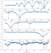 |
Fig. A.1. Merged X-shooter spectrum of J22564-5910, showing the UVB arm. Spectral features of interest of the star are indicated by vertical red-dashed lines. The sharp interstellar Ca lines are marked in black. The location of the Mg I triplet is marked, but the quality of the spectra is not sufficient to confirm its detection. |
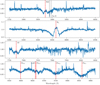 |
Fig. A.2. Merged X-shooter spectrum of J22564-5910, showing the VIS arm. Spectral features of interest of the star are indicated by vertical red-dashed lines. The interstellar sharp sodium doublet is marked in black. The Pachen H lines are indicated by ‘Pann’. The location of the λ8662 line of the Ca IR triple is shown in the bottom row. The other two lines of the Ca IR triplet are not visible in the spectrum. |
Appendix B: Nearby companion
Images show a relatively nearby star (Gaia EDR3 6491685391064878080) at a separation of ∼ 17.2 arcsec. The parallax and proper motion of both stars are given in Table B.1. The parallax of the nearby star is nearly identical to that of J22564–5910, 1.58 ± 0.02 and 1.52 ± 0.13 for J22564–5910 and the companion, respectively. At a distance of 635 pc, the separation between both systems is roughly 8300 AU, which is fairly common for sdBs with wide astrometric companions (Igoshev et al. 2020). The SED of the companion star hints at a very cool small star (Teff < 3500K, R ∼ 0.5 R⊙). This companion star is too far away and too faint (Gaia G = 18.4 mag, 2MASS J = 15.7 mag) to influence the observations of J22564–5910.
Parallax and proper motion of J22564–5910 and its nearby companion, obtained from Gaia EDR3.
The difference in the proper motion between J22564–5910 and the companion corresponds to a physical velocity of 58.7 km/s. At the same time, the escape velocity for a 0.5+0.5 M⊙ binary with a separation of 8300 AU is equal to ∼0.33 km/s. This strongly suggests that the objects are unbound from each other. When tracing their galactic orbits backwards, they cross but not at the same time. It is possible to interpret this as a scenario where the system started out as a hierarchical triple. The inner binary merges to form the sdB, and due to the merger process, the outer companion gets ejected. In this case, the distance and velocity difference can be used to estimate the time passed since the merger. Assuming the trajectories of the two stars share the same origin, the travel time would be about 670 yr. J22564–5910 would then be observed very early after the merger. However, since the orbits do not place both components at exactly the same position and at the same time, it is possible that this is just a chance encounter.
The presence of a nearby optical companion can indicate a possible triple origin of the system, (e.g. Toonen et al. 2016). In this case, the MS companion would be ejected during a dynamical triple interaction phase between the MS companion and two He-WDs. J22564–5910 would then form as a remnant from a merger of these two He-WDs. In this case, the system would have to be only ∼700 yr old, which might explain the presence of disc-like CM or the strong magnetic field of the sdB, which would then be driven by trace accretion. Such a dynamical triple interaction could have been triggered by mass transfer between an RGB star and a He-WD companion. Mass loss from the more massive red giant would widen the inner orbit and, if the tertiary companion were sufficiently close, drive the system made of the tertiary MS star, the He-WD accretor, and the core of the red giant towards a chaotic dynamical triple interaction phase (Mardling & Aarseth 1999; Toonen et al. 2020). At the end of this phase, the He-WDs would merge, leaving an unbound MS companion. This scenario requires that some red giant material lost during the mass transfer phase would remain between J22564–5910 and its companion, not bound to either star in particular, which may possibly be detectable with ALMA. Similarly, this scenario requires that in RV, the MS companion is moving away from J22564–5910.
All Tables
Photometry of J22564–5910 collected from SKYMAPPER, Gaia, APASS, 2MASS, and WISE.
Observing date, exposure time, signal-to-noise ratio (S/N), and resolution of the reduced spectra of the UVES and X-shooter observations of J22564–5910.
Galactic orbit calculation of J22564–5910: input parameters for GALPY together with the resulting Galactic orbital parameters.
Field estimates for the three spectra in which three Zeeman components can be identified for the Hβ, Hγ, and Hδ lines.
Parallax and proper motion of J22564–5910 and its nearby companion, obtained from Gaia EDR3.
All Figures
|
Fig. 1. Photometric SED of J22564–5910 obtained from literature photometry. The best-fitting model is shown with solid black line, with the contribution of the sdB shown with a blue-dashed line. The contribution of the IR excess, likely from a disc, is shown with a green-dashed line. The bottom shows the O–C between the observations and the best fitting model. |
| In the text | |
|
Fig. 2. Spectral trail of hydrogen and helium lines visible in the spectrum of J22564–5910. The rest wavelength of each line is shown in red dotted line. On the top left plot the Mg IIλ 4483 line is marked in green. On the bottom right plot the location of RK is indicated in blue dash-dotted line (see Sect. 6.1). The spectra are shown in order of observations – the time since the first spectrum is shown on the y axis. The bottom three spectra were taken with UVES, while the top three spectra were taken with X-shooter. The first two UVES spectra were taken back to back. The axes on the bottom of the plot shows wavelength, while that on the top shows velocity compared to the rest wavelength. |
| In the text | |
|
Fig. 3. Radial velocities of J22564–5910 as determined from the wings of the hydrogen lines. The first three measurements in blue are obtained from the UVES spectra, while the latter measurements are from the X-shooter spectra. Apart from one measurement, all RVs are consistent with no variation. |
| In the text | |
|
Fig. 4. Top: periodogram (grey) of the TESS light curve for J22564–5910. The light blue line is the re-calculated periodogram after the first whitening cycle. The red-dashed line indicates log(FAP) = − 4. Bottom: phase-folded (at the 0.069764 d period, respectively) and averaged (every 50 points) TESS light curve. |
| In the text | |
|
Fig. 5. Magnetic field estimate for the last obtained X-shooter spectrum. We note that Hδ, Hγ, and Hβ are shown from left to right. The observed spectrum is shown as a thin black line; a smoothed spectrum, restricted to the region where the Zeeman components were fitted, is shown as a thicker line. The fits to each Zeeman component are shown as red-dashed lines. The models of Schimeczek & Wunner (2014) are shown in grey, with the averaged separation including higher-order terms shown in blue, and the corresponding field strength shown on the right-hand side. The estimate for this spectrum was 660 ± 62 kG. |
| In the text | |
|
Fig. 6. Illustration for the structure of the system for the magnetic interpretation. The spinning subdwarf (in blue) generates a dipolar magnetic field around it, which is not necessarily aligned with the spin. The wind material in the innermost region, within Kepler radius RK, has no centrifugal support and can fall freely back onto the star, thus forming a dynamical magnetosphere. The material between the Keplerian co-rotation radius RK and the Alfvén radius RA has centrifugal support. It cannot fall back onto the star, thus forming a much denser rigidly rotating magnetosphere. The illustration is inspired by Petit et al. (2013). |
| In the text | |
|
Fig. 7. Same as Fig. 2, but spectral trail of lines likely to originate in the circumstellar material visible in the spectrum of J22564–5910. For the Ca II line, the UVES spectra show only noise and they are not shown here. The other two components of the Ca IR triplet are not visible in the spectra. |
| In the text | |
|
Fig. 8. Synthetic spectra of the Hβ line compared with the observations. The theoretical spectrum of the star without the disc is shown in green. The theoretical spectrum of the star + disc is shown in blue. The observed spectrum is shown in red. More details may be found in Sect. 6.2. |
| In the text | |
|
Fig. 9. Expected reflection effect for a typical dM companion at different inclination angles as a function of orbital period. The solid red line shows the detection limit of TESS. On the right axis, the known period distribution of sdB+dM binaries is shown in blue. In black, the period distribution of sdB binaries with an unknown companion (low mass MS or WD) is shown. The period distributions were taken from Kupfer et al. (2015). |
| In the text | |
|
Fig. A.1. Merged X-shooter spectrum of J22564-5910, showing the UVB arm. Spectral features of interest of the star are indicated by vertical red-dashed lines. The sharp interstellar Ca lines are marked in black. The location of the Mg I triplet is marked, but the quality of the spectra is not sufficient to confirm its detection. |
| In the text | |
|
Fig. A.2. Merged X-shooter spectrum of J22564-5910, showing the VIS arm. Spectral features of interest of the star are indicated by vertical red-dashed lines. The interstellar sharp sodium doublet is marked in black. The Pachen H lines are indicated by ‘Pann’. The location of the λ8662 line of the Ca IR triple is shown in the bottom row. The other two lines of the Ca IR triplet are not visible in the spectrum. |
| In the text | |
Current usage metrics show cumulative count of Article Views (full-text article views including HTML views, PDF and ePub downloads, according to the available data) and Abstracts Views on Vision4Press platform.
Data correspond to usage on the plateform after 2015. The current usage metrics is available 48-96 hours after online publication and is updated daily on week days.
Initial download of the metrics may take a while.