| Issue |
A&A
Volume 655, November 2021
|
|
|---|---|---|
| Article Number | A48 | |
| Number of page(s) | 17 | |
| Section | Catalogs and data | |
| DOI | https://doi.org/10.1051/0004-6361/202038318 | |
| Published online | 16 November 2021 | |
An XMM–Newton catalogue of BL Lacs⋆
1
Quasar Science Resource S.L. for the European Space Agency (ESA), European Space Astronomy Centre (ESAC), Camino Bajo del Castillo s/n, 28692 Villanueva de la Cañada, Madrid, Spain
e-mail: This email address is being protected from spambots. You need JavaScript enabled to view it.
2
European Space Agency (ESA), European Space Astronomy Centre (ESAC), Camino Bajo del Castillo s/n, 28692 Villanueva de la Cañada, Madrid, Spain
3
Serco Gestión de Negocios SLU for the European Space Agency (ESA), European Space Astronomy Centre (ESAC), Camino Bajo del Castillo s/n, 28692 Villanueva de la Cañada, Madrid, Spain
4
Center for Interdisciplinary Exploration and Research in Astrophysics (CIERA) and Department of Physics and Astronomy, Northwestern University, 1800 Sherman, Evanston, IL 60201, USA
Received:
1
May
2020
Accepted:
2
July
2021
Abstract
Aims. We present an XMM–Newton catalogue of BL Lac X-ray, optical, and UV properties based on cross-correlation with the 1151 BL Lacs listed in the fifth edition of the Roma–BZCAT.
Methods. We searched for the X-ray counterparts to these objects in the field of view of all pointed observations in the XMM–Newton archive over nearly 20 years of mission. The cross-correlation yields a total of 310 XMM–Newton fields which correspond to 103 different BL Lacs. We homogeneously analysed data from the three EPIC cameras (X-ray) and OM (optical/UV) using the XMM–Newton SAS software, and produced images, light curves, and spectral products for BL Lacs detected in any of the three EPIC cameras. We tested two different phenomenological models, log parabola and power law, with different variations of the absorbing column density and extracted their parameters. We derived time-variability information from the light curves following well-established statistical methods and quantified variability through statistical indicators. OM magnitudes and fluxes were computed wherever possible.
Results. We see that the log parabola model is preferred over the power law model for sources showing higher fluxes, which might indicate that curvature is intrinsic to BL Lacs and is only seen when the flux is high. We present the results of our analysis as a catalogue of X-ray spectral properties of the sample in the 0.2–10 keV energy band as well as in the optical/UV band. We complete the catalogue with multi-wavelength information at radio and γ-ray energies.
Key words: BL Lacertae objects: general / galaxies: active / X-rays: galaxies / catalogs
Tables B.1–B.4 and C.1 are only available at the CDS via anonymous ftp to cdsarc.u-strasbg.fr (130.79.128.5) or via http://cdsarc.u-strasbg.fr/viz-bin/cat/J/A+A/655/A48
© ESO 2021
1. Introduction
According to the unified scheme of active galactic nuclei (AGNs), a blazar is considered to be a radio-loud AGN that displays highly variable, beamed, non-thermal emission covering a broad wavelength range from radio to γ-ray energies (Urry & Padovani 1995). The properties of the blazar non-thermal emission suggest a relativistic origin in a jet oriented at a small angle to our line of sight (Blandford & Rees 1978). The blazar class encompasses BL Lacertae (BL Lac) objects and flat-spectrum radio quasars (FSRQs). The most striking difference between the two lies in their optical spectra, with the former showing weak or no emission or absorption lines (EW < 5 Å, Stickel et al. 1991) and the latter strong broad emission lines. One difficulty in the study of BL Lacs is indeed that in many cases it is not possible to measure any redshift because of a lack of features in their optical spectra (see e.g., Álvarez Crespo et al. 2016). Blazars, and in particular BL Lacs, are very strong γ-ray emitters, being the most numerous extragalactic sources at high energies (see Acero et al. 2015; Nolan et al. 2012; Abdo et al. 2010a).
Observationally, the spectral energy distribution (SED) of blazars in a νFν representation shows two broad distinctive peaks (see e.g., Padovani & Giommi 1995). The most widely accepted interpretation of the first bump of the SED is that it is due to synchrotron radiation of relativistic electrons moving along the jet. Different models offer alternative solutions as to the origin of the second spectral component, namely leptonic or hadronic. In the leptonic model, the second peak is the result of inverse Compton (IC) scattering of low-energy photons to high energies by the very same electrons that produce the synchrotron peak. The up-scattered photons can be the synchrotron photons themselves (self-synchrotron Compton model, SSC; Ghisellini 1999; Ghisellini et al. 1992) or ambient photons of different origins (external Compton model, EC; see review Sikora et al. 2001). On the other hand, hadronic models establish the origin of the second peak as synchrotron emission from high-energy protons or photoproduction induced by accelerated protons (see e.g., Mannheim 1996; Aharonian 2000; Mücke et al. 2003). Blazars presenting the first peak in their SED at UV/X-ray energies ( Hz) are referred to as high-synchrotron peaked blazars (HSPs). For intermediate-synchrotron peaked blazars (ISPs), the synchrotron peak frequency lies at 10
 Hz. Those blazars presenting their synchrotron peak frequency at
  Hz, between radio and optical wavelengths, are known as low-synchrotron peaked blazars (LSPs; Abdo et al. 2010b). BL Lacs can belong to all these three categories, while most FSRQs have been classified as LSPs.
Fossati et al. (1998) showed that the SED in blazars is correlated with the bolometric luminosity, forming the so-called blazar sequence. As the bolometric luminosity increases, blazars become redder, that is, their two bumps in the SED show smaller peak frequencies and the Compton peak becomes increasingly dominant. Ghisellini et al. (1998) interpret this as a result of the different amounts of radiative cooling suffered by electrons in different sources. On the other hand, Giommi et al. (2012) consider that this blazar sequence is most likely a selection effect due to the selection of sources from radio- and X-ray-flux-limited samples. Using Monte Carlo simulations to populate the blazar sequence, these latter authors consider that BL Lacs could not be plotted at high luminosity and high  ; not because these objects do not exist but rather because it is not possible to measure their redshifts and therefore it is not possible to estimate their luminosities. Ghisellini et al. (2017) used the Third Large-Area telescope AGN Catalogue (3LAC, Ackermann et al. 2015) to revisit the blazar sequence. They constructed their average SED using γ-ray luminosities, finding an anti-correlation with the synchrotron peak frequency. Their new results support the blazar sequence scenario.
The Fermi Gamma-ray Space Telescope launched in 2008 has revealed more than 5000 sources. With a sky density of ∼0.1 sources deg2, blazars and particularly BL Lacs dominate the γ-ray sky and constitute more than 75% of the associated sources in all releases of the Fermi catalogues (1FGL, Abdo et al. 2010a), (2FGL, Nolan et al. 2012), (3FGL, Acero et al. 2015) and (4FGL, Abdollahi et al. 2020). However, all these catalogues present a fraction of about one-third of the sources as unassociated or unknown. The discovery that blazars occupy a narrow region in the WISE IR colour-colour space, the so-called WISE blazar strip (WBS, Massaro et al. 2011; D’Abrusco et al. 2012), has been used to search for blazar-like sources within the positional uncertainty regions of the unidentified or unassociated γ-ray sources (UGSs) leading to many new blazar candidates (D’Abrusco et al. 2014; D’Abrusco et al. 2019; Álvarez Crespo et al. 2016; de Menezes et al. 2020).
Several studies have proven that BL Lacs exhibit high amplitude and rapid variability on timescales that can vary from hours to months, and so the nature of the X-ray spectra in BL Lacs is variable and shows a complex behaviour (see e.g., Zhang et al. 2006; Falcone et al. 2004; Brinkmann et al. 2005). The shape of the X-ray spectrum can provide information that can be used to reveal the emission components, as X-ray emission probably originates in the inner parts of the relativistic jet. The transition in the SED between synchrotron and IC in BL Lacs is located with the X-rays, and therefore characterising the spectra in this band where both processes can contribute to the X-rays is of special relevance. When the mechanism responsible for the emission is synchrotron, we observe a steep power-law energy distribution (α > 1, F ∝ ν−α) due to the tail of its spectrum, while if IC is the dominant process we observe a flat component (α < 1). In the SED of HSPs, the X-ray radiation comes from the high-energy end of the synchrotron, whereas in LSPs it comes from Compton scattering.
Here we present a catalogue that compiles 310 observations corresponding to 103 different BL Lacs observed with XMM–Newton over nearly 20 years of operations. We make use of the fifth edition of the catalogue Roma-BZCAT (‘BZCAT’ hereafter, Massaro et al. 2015), which constitutes the most comprehensive list of blazars known to date and is based on multi-frequency surveys and information reported in the literature. BZCAT contains 3561 sources, of which 1151 are confirmed BL Lacs. Here we report those BL Lacs observed by XMM–Newton and reported in the archival public observations1 up to September 2019. We fit six different models to each XMM–Newton source where sufficient counts are available to produce a spectrum: two different phenomenological models, log parabola and power law, each with three different flavours for the absorbing column density. We study their parameters and choose the best-fit model. The catalogue includes light curves, derived variability parameters, and optical and ultraviolet (UV) information when available.
The paper is organised as follows. In Sects. 2 and 3 we describe the sample selection with observations and data analysis, respectively. In Sect. 4, we describe the catalogue, the products and how to access it. In Sect. 5 we present and discuss the spectral properties and the results of the best-fit model, and in Sect. 6 we present our conclusions.
Unless otherwise stated, we assume a flat ΛCDM cosmology with a Hubble constant H0 = 70 km s−1 Mpc−1, total matter density Ωm = 0.27 and dark energy density ΩΛ = 0.73. Magnitudes throughout this paper refer to the AB magnitude system (Oke 1974).
2. Sample selection
The sample we present here is the result of a cross-correlation between the 1151 BL Lac subsample given in the fifth version of the Roma–BZCAT and all the pointed science public observations available in the XMM–Newton archive. Overall, observations covered by the catalogue include the period from March 2000 to September 2019. Calibration observations cover up to September 2020. Their cross-correlation with the XMM–Newton archive yields a total of 310 XMM–Newton observations that contain a BZCAT source, corresponding to 103 different BZCAT sources. The 310 XMM–Newton observations are selected by searching in squares of sizes Sx = 0.5°/cos(Dec), Sy = 0.5°, centred at the positions of the BZCAT sources to see if the centre of an XMM–Newton observation is contained within this box, which is equivalent to saying that the BZCAT source is contained within any field of view of an XMM–Newton observation. Figure 1 shows the sky distribution in equatorial coordinates of the BZCAT BL Lacs and those present in our XMM–Newton BL Lac Catalogue. Because of the selection procedure, the sample is heterogeneous, certainly not complete, and sources are observed in different epochs.
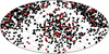 |
Fig. 1. Equatorial coordinates of the BL Lacs from BZCAT, indicated as black points. Red crosses mark the distribution of those sources contained in the catalogue of XMM–Newton BL Lacs. |
In the XMM–Newton BL Lac catalogue, 101 of the 103 different sources are detected in the EPIC cameras (EPIC-MOS and EPIC-pn, respectively) as described in Sect. 3. The BL Lac 5BZBJ2214+0020 (1/103) is detected in one pointing and undetected in another. For the remaining (2/103) BL Lacs, flux upper limits are provided. The BL Lacs detected in our catalogue are a combination of XMM–Newton targets (41/101) and serendipitous objects (60/101) found anywhere within the field of view of the EPIC cameras. Within the 41 sources that are targets, 4 sources are the target of observations in some observations and field sources in other observations. Any source lying more than 0.5′ from the nominal XMM–Newton pointing is considered serendipitous. All calibration sources are considered as targets, even if displaced from the nominal pointing.
We classify the BL Lacs according to the estimated value of the synchrotron peak frequency  calculated in the observed frame as defined in Sect. 1, following the nomenclature used in the Fourth Large-Area Telescope AGN Catalogue (4LAC, Ajello et al. 2020). For some BL Lacs these values are reported in the 4LAC, while for the rest of the sources we build their SEDs source by source using the ASDC SED Builder Tool2, which collects all available data in the literature. We estimate the peak of the synchrotron emission
  using a third-degree polynomial fit on the low-energy hump:
 (1)
(1)
where the error associated with  is typically ∼0.5 due to the use of non-simultaneous broadband data (Kapanadze 2013).
With this criteria, about 48% of the BL Lacs in the XMM–Newton catalogue are classified as HSPs, 26% as ISPs, and 21% as LSPs. For the remaining fraction of sources, it is not possible to make a classification because of a lack of sufficient broadband data to perform an adequate fit.
3. Observations and data analysis
3.1. Instrument and observations
The XMM–Newton observatory carries several coaligned X-ray instruments: the European Photon Imaging Camera (EPIC) and two reflection grating spectrometers (RGS1 and RGS2, Jansen et al. 2001). The EPIC cameras consist of two metal-oxide semiconductors (EPIC-MOS, Turner et al. 2001) and one pn junction (EPIC-pn, Strüder et al. 2001) CCD array, which have a ∼30′ field of view (FOV) and can offer 5–6″ spatial resolution and 70–80 eV energy resolution in the 0.2–10 keV energy band. XMM–Newton also has a co-aligned optical/UV telescope of 30 cm in diameter (Optical Monitor, OM), providing strictly simultaneous observations with the X-ray telescopes (Mason et al. 2001). It has three optical and three UV filters, with effective wavelengths V: 543 nm, B: 450 nm, U: 344 nm, UVW1: 291 nm, UVM2: 231 nm, and UVW2: 212 nm covering a 17 × 17 arcmin2 FOV (but with the actual imaged sky area being dependent on the user-chosen mode) and a point spread function (PSF) of less than 2″ FWHM –depending on filter– over the full FOV (Rosen 2020).
The information on the 310 XMM–Newton observations reported in this work comes mainly from the EPIC detector. EPIC observations present in this catalogue have been taken under timing and imaging mode, this latter in combination with different window modes (Small Window, Large Window, and Full Frame) and filters (Thick, Medium, and Thin). EPIC data are available for all observations in at least one of the three cameras. For 35% (36/103) of the objects, several observations exist. Observing times per observation range between 2.7 ks and 144 ks (see Fig. 2), and observing times per object range between 2.7 ks and 2.2 Ms, spanning several years in some cases.
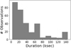 |
Fig. 2. Distribution of the exposure time (in ks) of single observations included in the catalogue of XMM–Newton BL Lacs. |
Data provided by the OM exist for 45% (46/103) of the objects in at least one of the filters. For 8 objects, data exists in all six filters (three optical and three UV). For 12 objects, there are data in all three optical filters, and for 13 there are data in all three UV filters. For 26 objects there are data in at list one optical and one UV filter. For 5 objects, no OM data are available due to the presence of bright objects in the field of view.
The following sections describe the EPIC data-reduction procedure.
3.2. Data reduction
Our sample has been uniformly analysed using the XMM–Newton standard Science Analysis System (SAS, v18.0.0; Gabriel et al. 2004) and most updated calibration files. Different observations of the same source are not combined for any purposes, including source detection. If several exposures exist for any given observation of a source, then the one with the longest exposure time is used. Event lists are produced for the three EPIC cameras following the standard SAS reduction procedure. Periods of high-background activity are removed following the standard method (Lumb et al. 2002), that is, monitoring the rate of events with pattern ‘0’ and energies > 10 keV (the limits that define the good time intervals (GTIs) are defined by background rates EPIC-pnrate < 1.0 cts/s−1 and EPIC-MOSrate < 0.8 cts/s−1).
EPIC-MOS1 exposures taken in TIMING mode contained in our data sample are discarded and not used in our analysis. Details explaining why this is the case can be found in the EPIC Status of Calibration and Data Analysis; latest update Oct 2019 (Smith 2019).
We use the standard omichain SAS task to analyse OM data. The processing chain performs source detection and computes rates and instrumental magnitudes as well as fluxes for every source detected.
In the following sections we highlight the main analysis steps needed to go from EPIC source detections (3.2.1), through coordinate corrections (3.2.2), and source cross-match (3.2.3) to end with the extraction of the catalogue products (3.2.4).
3.2.1. Source detection
The source-detection algorithm is applied only to exposures taken in IMAGING mode. If the exposure time is less than 100 s in any given EPIC exposure after GTI filtering, the exposure is not considered for source detection and the source is flagged as not detected. All the TIMING exposures in our data sample contain a source, so they are flagged as detections by default.
The GTI-filtered event-detection criteria have to be established for the EPIC cameras. For this purpose, images with a bin size of 40 pixels bin−1 are produced in five different energy ranges (EPIC-pn: 300–500, 500–2000, 2000–4500, 4500–7500, 7500–12 000 eV; EPIC-MOS: 200–500, 500–2000, 2000–4500, 4500–7500, 7500–12 000 eV). These images are used by the SAS task edetect_chain to establish source detection. This task is run simultaneously over the five energy bands and each camera independently. A positive detection requires a detection likelihood threshold of 10. A radial statistical error is associated to every detected source, computed as  , where RAerr and Decerr are the 1σ statistical uncertainties in the derived RA and Dec coordinates respectively.
3.2.2. Source position rectification
Subsets of objects within the XMM–Newton FOV, extracted from large astrometric reference catalogues, are used to rectify the source positions derived by edetect_chain. Before this is done, the SAS task srcmatch is used to create a unique EPIC source list using information from all EPIC cameras in which the source has been detected. This unique list contains average source information, such as fluxes. Within this unique list, the associated RA and DEC are an average of those found independently for each camera, and the positional error is a combination of statistical and systematic errors. For reference, the average 1σ positional error for the whole Fourth XMM–Newton Serendipitous Source Catalogue (4XMM, Webb et al. 2020) is better than ∼1.7″, with a standard deviation of 1.4. As for the systematic errors, the relative astrometry within each camera is accurate to within 1.5″ over the full FOV.
The SAS task catcorr is run over the unique EPIC source list to update the sky coordinates by cross-matching them with up to three reference external catalogues, (i) the USNO B1 catalogue (Monet et al. 2003), (ii) the 2MASS catalogue (Skrutskie et al. 2006), and (iii) the SDSS (DR9) catalogue (Ahn et al. 2012), to find optical or infrared (IR) counterparts and to find the small frame shifts or rotations that optimise the match. If sufficient matches are found within the FOV to optimise the correction, these shifts are then applied to the positions of all the EPIC sources in the field. The average 1σ field correction is of the order of 2.5″. Where catcorr fails to obtain a statistically reliable result, the associated systematic error is assumed to be 1.5″.
The average (over all EPIC cameras) and external catalogue rectified sky coordinates are used as the coordinates of the XMM–Newton X-ray sources that make up our catalogue. The catalogue includes the coordinates XMM_RA_NOCORR, XMM_DEC_NOCORR, and XMM_RADEC_ERR_NOCORR before astrometric rectification, and XMM_RA, XMM_DEC, and XMM_RADEC_ERR after astrometric rectification. Two further columns in the catalogue, AstCorr and PosCorr, identify if astrometric rectification has been applied and if the fitting was successful in providing updated coordinates.
3.2.3. Catalogue cross-match
Once we have the XMM–Newton sources with rectified positions, a positive match with a BZCAT source is considered if:
 (2)
(2)
where distance refers to the distance between the XMM–Newton and BZCAT source in units of arcsec; σBZCAT is the reported positional uncertainty of the order of 1″; and σXMM the estimated XMM–Newton positional uncertainty, a combination of  , the statistical and systematic uncertainty in the XMM–Newton position, where σSTAT = 1.5″ on average, and σSYS ∼ 1.5″. This translates to an average distance no greater than ∼5″ (2σ) between the XMM–Newton detected source and the BZCAT source in order to consider the X-ray source a match of the BZCAT one.
In summary, if the XMM–Newton detected source is within ∼5″ of the BZCAT one, we consider the X-ray source to be a positive match. With this criteria, the cross-match yields 307/310 XMM–Newton observations with an identified BZCAT source, corresponding to 103 different BZCAT sources.
3.2.4. Catalogue product extraction
Once a positive identification of the X-ray source has been established, source and background extraction regions are defined to derive source light curves and spectra.
For IMAGING mode, the source region is chosen to be circular around the source centroid with a minimum radius of 20″ and limited to a maximum of 40″, whereas the background region is an annulus around the source region with inner radius rmin = 60″ and outer radius rmax = 120″. This selection ensures that the source region is greater than the PSF of the instrument (4–6″) and that the background region is away from any possible source contamination. Additional X-ray sources in the background region are masked out by removing those with a detection likelihood greater than 50. The SAS task eregionanalyse is used to maximise the S/N calculated from the source counts, the encircled energy fraction, and the background counts to give the optimum source radius and source centroid. If eregionanalyse cannot find an optimal extraction radius, the exposure is discarded by our analysis.
An exception to the above rule for IMAGING mode exposures is the definition of background extraction regions taken from exposures in Small Window mode. To avoid contamination from the bright central source, for EPIC-pn the background region is taken from a circular region from a corner of the available window rather than from an annulus around the source. The circular background-extraction region has a radius of 37.5″. For EPIC-MOS, the background region is taken from a circular region from one of the outer CCDs, in particular from CCD5. The radius of the background-extraction region is 120″. Figure 3 illustrates how extraction regions are selected for the two IMAGING mode EPIC exposures, Full Frame and Small Window.
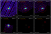 |
Fig. 3. Top: EPIC IMAGING Full Frame mode source (orange) and background (red) extraction region definition for the source 5BZBJ0333-3619. Left panel: PN, middle panel: MOS1, and right panel: MOS2 cameras. Bottom: EPIC IMAGING Small Window mode source (orange) and background (red) extraction region definition for the source 5BZBJ0326+0225. |
For TIMING mode exposures in EPIC-pn, both source and background are extracted from boxes in RAWX versus RAWY. The source region is defined from a box of 16 × 199 RAW X,Y units with centre Xcentre = ⟨RAWX⟩ and Ycentre = 101. The background is extracted from a box of 16 × 199 RAW X, Y units with centre Xcentre = 8.5 and Ycentre = 101. The background box is moved along RAWX from the edge of the detector by 0.5 units.
For TIMING mode exposures in EPIC-MOS, the source and background are extracted from boxes in RAWX versus TIME. The source region is defined from a box of 60 RAWX units and full time (Exposure) interval with centre Xcentre = ⟨RAWX⟩ and Ycentre = T_Start + ⟨Exposure⟩/2.. The background is extracted from a box of 20 RAWX units with centre Xcentre = 264.0 and Ycentre = T_Start + < Exposure > /2, where T_Start is the exposure start time.
3.2.5. Pile-up evaluation and correction
For IMAGING mode exposures, the presence of ‘pile-up’ is evaluated. To test for pile-up we derived the source+background count rate extracted from a circle around the source of 60″ (this radius contains about 95% of the PSF). To establish the presence of pile-up, these count rates are compared against pile-up limits given in Table 2 of Jethwa et al. (2015) which are in line with the following criteria: a conservative limit where 2%–3% flux loss and less than 1% spectral distortion is incurred, and a tolerant limit allowing for 4%–6% flux loss and 1%–1.5% spectral distortion. These limits are a function of the EPIC observing submodes and are available for Full Frame, Large Window, and Small Window modes, both for EPIC-pn and EPIC-MOS. If the submode is outside these values, a tag UNK is used to mark in the catalogue the presence of pile-up. The number of IMAGING mode exposures in the catalogue where pile-up is present is: 82/238 for EPIC-pn, 102/253 for EPIC-MOS1, and 114/284 for EPIC-MOS2.
An attempt is made to reduce the pile-up only below the 2%–3% flux loss limit. This is only done to extract spectral products, the correction is not applied to extract light-curve products. The procedure involves iteratively removing circles around the source centroid, starting with a radius of 10″ and taking increasing steps of 5″ until the pile-up is below the 2%–3% flux loss limit. In every step, the presence of pile-up is tested up to a maximum removal radius of 30″ (about 90% of the PSF). If at this point pile-up is still present, no more corrections are attempted as no PSF would be left to extract any meaningful spectral products. However, rather than throwing out the exposure, spectral products are still derived from the full source region, and so care has to be taken in interpreting the spectral results derived from these exposures. Overall, the pile-up correction worked for 54/82 EPIC-pn exposures, 56/102 EPIC-MOS1 exposures, and 67/114 EPIC-MOS2 exposures where pile-up was present. Table 1 collects the list of 53 observations where there is at least one exposure where pile-up could not be removed. Of these, 25 observations contain no exposures free of pile-up, where 24 of these 25 correspond to observations of MRK 421 (5BZBJ1104+3812). In the remaining 28, it is possible to find at least one exposure that is free of pile-up. In summary, out of the 310 observations contained in the catalogue, 25/310 suffer from irrecoverable pile-up effects.
53 observations with at least one EPIC exposure where pile-up is present and cannot be corrected.
3.2.6. Quality flags
Several quality flags are checked before catalogue products are extracted. First, we check whether the GTI filtered exposure time is greater than 100 s; if it is not, the analysis of the exposure stops here. If there is a positive detection, the next step is to establish the presence of pile-up, and if present, whether it can be corrected as described in Sect. 3.2.5. For the light-curve generation, a minimum of 500 s is required. Finally, the spectrum has to contain at least 300 counts to ensure a minimum quality spectral fitting.
3.3. Catalogue products
The catalogue products include EPIC images, light curves, and spectral products. These are obtained from the GTI-filtered event lists as described in Sect. 3.2. Light-curve and spectral products are acquired from the source- and background-extraction regions as described in Sect. 3.2.4. When available, OM images together with magnitudes and fluxes are given too. All products have been visually screened to check for problems. In the following sections, we describe how individual products are obtained.
3.3.1. Image generation
Images are produced for all individual IMAGING mode exposures in sky coordinates with a bin size of 40 units. These images are used for source detection and are available in five energy ranges (EPIC-pn : 300–500, 500–2000, 2000–4500, 4500–7500, 7500–12 000 eV; EPIC-MOS: 200–500, 500–2000, 2000–4500, 4500–7500, 7500–12 000 eV). Thumbnail true colour images are produced around the X-ray source, as seen in Fig. 4 (Events in red: 0.5–4.5 keV, green: 4.5–7.5 keV, blue: 7.5–12.0 keV).
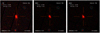 |
Fig. 4. EPIC IMAGING mode thumbnail true colour images around the X-ray source 5BZBJ0613+7107 marked by a red cross (Events in red: 0.5–4.5 keV, green: 4.5–7.5 keV, blue: 7.5–12.0 keV). Blue circles mark other X-ray sources in the field. |
3.3.2. OM image and source information
OM images and source information are obtained via the SAS task omichain when OM exposures are available. This SAS perl script reduces OM Imaging mode data and produces individual mosaiced sky images and combined source lists with flux and magnitude information. For the purpose of this work, omichain is run with the optional parameters processmosaicedimages and usecat set to true in order to maximise the astrometric accuracy of the detected sources and provide the deepest level of imaging product (mosaiced sky images) when possible.
omichain comprises a number of SAS tasks. The imaging pipeline first processes the image for individual exposures, producing a set of OM imaging-mode products including the list of detected sources per exposure through the omdetect SAS task. In cases where more than one exposure is available per filter, the ommosaic SAS task generates a mosaic sky image per filter as a combination of the individual exposures. omsrclistcomb then combines the source lists corresponding to the available individual exposures. Finally, ommergelists combines all the available source lists for the different filters and produces an associated region file. Source quality flags for OM are one of the outputs of omichain and are included in Table B.3 of the catalogue (see Sect. 4.1).
The main OM information contained in our catalogue is magnitudes and fluxes in any of the six passbands where the source is detected. This information is extracted from the observation source list produced by omichain, which includes the results of the combination of multiple exposures and different extraction apertures. These apertures are used to derive fluxes and are not fixed, but vary between 3″ and 6″. Fluxes provided in our catalogue are not extinction corrected. For a more detailed discussion on apertures used to extract fluxes and how to deal with extinction corrections we refer the readers to Page et al. (2012).
For the astrometric corrections of the detected sources, omsrclistcomb identifies if a USNO catalogue file is available, and if so corrects the astrometry –depending on whether there are sufficient matches of OM detections with USNO objects–in order to account for any offset between the OM and USNO source adding the columns RA_CORR and Dec_CORR to the combined master source list. This final list is then cross-matched with the coordinates of our source of interest. We follow the same procedure as described in Sect. 3.2.3 for the EPIC cameras. In this case, we consider  the estimated positional uncertainty, a combination of statistical and systematic uncertainties in the OM position, where σSTAT ranges from 0.05 to 2.57″, with a mean position uncertainty of 0.68″ (Page et al. 2012) and σSYS ∼ 0.7″ (Rosen 2020). In a similar manner as with EPIC sources, this implies that a significant positive match is found if the BZCAT source lies within ∼3″ of the OM source. This is a purely geometrical approach based on the statistical coordinates of the OM source and no attempt has been made to use the extent of the OM source. The observation source lists contain information relative to the extension of the source. This information is not contained in our catalogue.
3.3.3. Light-curve generation
Source and background light curves are produced in two energy ranges, Esoft = 0.2 − 2.0 keV and Ehard = 2.0 − 10.0 keV, over bins of 500 s. For TIMING mode exposures, the low-energy limit of the soft band light curve is set at 0.3 keV to avoid low-energy noise.
The SAS task epiclccorr is used to produce background-subtracted source light curves corrected for inefficiencies of the instrument (vignetting, chip gaps, PSF etc.) and time corrections (dead time, GTIs, etc.). A hardness ratio (Ehard/Esoft) light curve is also produced. The left panel in Fig. 5 shows a representative example of a generated light curve. Weighted average rates over the entire exposure are derived for the two energy bands and marked in the figure with a discontinuous line. Time bins below 15% effective exposure are identified (marked in red) and not used in the calculation of these average rates.
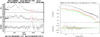 |
Fig. 5. Example light curve and spectra of 5BZBJ1221+2813. Left: EPIC-pn light curve in the 0.2–2.0 keV (top) and 2.0–10.0 keV (middle) bands and hardness ratio (bottom). Red symbols indicate those bins for which the effective exposure is below 15%. Right: combined spectral fit for EPIC-pn (black), EPIC-MOS1 (green), and EPIC-MOS2 (red) spectra corresponding to the power law with the two-absorption-component model. |
3.3.4. X-ray variability
We measure and quantify the source X-ray variability using the above-generated light curves for each exposure separately and over the two defined energy ranges (Esoft = 0.2–2 keV and Ehard = 2–10 keV). For both, we use the SAS task ekstest. The task uses the source and background time series to run several variability tests. Only bins within GTI intervals are used and bins containing null or negative values are eliminated.
The χ2 analysis is used to test the null hypothesis of a constant source rate, so that sources are reported as variable in Table C.1 when the χ2 probability is ≤10−5 in at least one exposure (Rosen et al. 2016). Both quantities, χ2 and χ2 probability, are included in the catalogue for every EPIC exposure and each energy range (Esoft and Ehard).
In addition, to quantify the scale of the variability, we use the fractional root mean squared variability amplitude Fvar (Nandra et al. 1997; Vaughan et al. 2003). This variable is the square root of the excess variance after normalisation by the mean count rate  . This is used as an estimator of the intrinsic source variance and is defined as:
 (3)
(3)
where S2 is the variance of the time series with N bins,
 (4)
(4)
and  is the mean square error of the time series. Fvar can be expressed as a percentage. The uncertainty in Fvar takes the form:
 (5)
(5)
Both quantities Fvar and ΔFvar are included in the catalogue for every EPIC exposure and each energy range (Esoft and Ehard).
3.3.5. Spectra generation
Source and background spectra are produced in the full energy range (0.2–10 keV) with an energy resolution of 5 eV. The SAS task backscale is used to calculate the area of the two regions used to extract the spectra. The corresponding response and ancillary files are also created. Finally, the spectra are re-binned in order to avoid over sampling the intrinsic energy resolution of the EPIC cameras by a factor larger than three while making sure that each spectral channel contains at least 25 background-subtracted counts to ensure the validity of Gaussian statistics and hence the applicability of the χ2 goodness-of-fit test.
3.3.6. Spectral fits
All the spectral fits are performed uniformly over our data sample with the XSPEC package version 12.10.1 (Arnaud et al. 1996). Spectral fits to the time-averaged spectra are performed in the energy range 0.3–10 keV in the case of IMAGING mode exposures and 0.6–10 keV in the case of TIMING mode exposures. Upper and lower confidence intervals are derived for relevant model parameters at the 68% level. For those fits where  , confidence intervals are not derived and instead parameter errors are reported at the 1σ level.
For all those instruments available within an observation where the source has been detected and passes the quality control flags (Sect. 3.2.6), we perform spectral fits and derive spectral parameters on an instrument-by-instrument basis and for the combined spectra of all those instruments.
Within XSPEC, fits are performed using C-statistics, while to test the goodness of fit, that is, how well the statistical model matches the data, χ2 statistics is used with standard weights (the statistical error given in the input spectrum). All spectra are fitted using the following two baseline models (Perlman et al. 2005):
– Power law:
 (6)
(6)
where Γ is the photon index. Within XSPEC, we use the pegpwrlw model, which also allows a simple extraction of the flux at a given energy value. In our case, we extract the X-ray flux at 5 keV.
– Log parabola:
 (7)
(7)
where Γ is the photon index and β measures the curvature of the parabola. E1 is a scale parameter (always frozen during the fitting procedure) which is set to the lower energy range used for fitting (Massaro et al. 2004). Within XSPEC, the logpar model is used.
Both models are applied using neutral cold absorption (e−σNH) where NH is the column density and σ is the photoelectric cross-section of the process according to Morrison & McCammon (1983). For NH, the following variations are tested:
– NH fixed to the Galactic column density, NH, Gal, during the fitting procedure. NH, Gal has been taken from the HI4PI, a full-sky HI survey based on EBHIS and GASS HI4PI Collaboration (2016). Within XSPEC, the tbabs model is used.
– NH is left free to vary during the fitting procedure. Within XSPEC, the tbabs model is used.
– A combination of two NH values is used, NH, Gal and NH, Z. The first fixed to the Galactic column density value during the fitting procedure and the second one used to account for any extra local absorption and left free to vary during the fitting procedure. This extra local component is a function of the source redshift. Within XSPEC, the ztbabs model is used.
Absorbed fluxes and luminosities (when redshifts are available) are derived inside XSPEC over the three bands used (soft, 0.2–2.0 keV; hard, 2.0–10.0 keV; and full energy band 0.2–10.0 keV). The right panel of Fig. 5 shows an example generated spectrum and the results of the combined spectral fit using the model power law with two absorption components, NH, Gal and NH, Z.
3.3.7. Flux upper limits
When no X-ray source is detected, flux upper limits at the BZCAT source location are derived over three different energy ranges (soft, 0.2–2.0 keV; hard, 2.0–10.0 keV; and full energy band 0.2–10.0 keV) at the 3σ confidence level. Flux upper limits are first derived in cts/sec from a 30″ radius region around the source location using the SAS task eregionanalyse using both a background and an exposure map. Count rates are converted afterwards to flux in units of 10−11 erg cm−2 s−1 using Energy Conversion Factors (ECFs) for each energy range (Mateos et al. 2009). These ECFs are derived from simulations assuming an absorbed power law model with NH = 3.0 × 10²⁰ hydrogen atoms cm−2 and Photon Index = 1.7. The ECFs used are camera-, energy band-, and filter dependent. When the redshift is available, upper limits to the luminosity are also derived. Only two sources in the catalogue do not show significant X-ray emission, namely 5BZBJ1721+6004 and 5BZBJ2036+6553. The source 5BZBJ2214+0020 is present in two XMM–Newton observations and in one of them (ObsId 0673000137) no significant emission is detected. Table 2 summarises these results.
XMM–Newton observations where no X-ray emission is detected at the location of the BZCAT source.
4. The catalogue
4.1. Description and access
The full catalogue is divided into four different tables. Tables B.1–B.4 report the description of the contents of each one, including the column name, units, and a short description of each column.
The first table is named “catalogue”, and contains 310 rows, one for each unique XMM–Newton observation, each characterised by an observation ID (ObsId) and 148 columns (Table B.1). Here, for each individual EPIC camera within an observation, we report different exposure and analysis properties, such as analysis quality flags (Sect. 3.2.6), source position rectification (Sect. 3.2.2), detection flags (Sect. 3.2.1), pile-up and pile-up-correction flags (Sect. 3.2.5), fit statistics (section 3.3.6), and flags to check whether light curves and spectral products are extracted (Sects. 3.3.3 and 3.3.5). The table also reports some source properties, such as count rates and variability parameters as defined in Sect. 3.3.4, also the flux extracted at 5 keV, the total flux, and the luminosity in the entire, soft, and hard energy bands extracted from the combined EPIC fit for the model power law with two absorption components (Sect. 3.3.6). Finally, detection flags and OM magnitudes and fluxes in the available filters are included (Sect. 3.3.2).
The next table of the catalogue of XMM–Newton BL Lacs is named “model” and reports information on the fits to the individual and combined EPIC exposures. The table contains 7440 rows and 62 columns as described in Table B.2. Here we report the best-fit model parameters obtained from the spectral fits (Sect. 3.3.6). The model table also includes background-subtracted counts (Sect. 3.3.3) and pile-up information (Sect. 3.2.5). For each ObsId, there are six rows corresponding to the results of the fits for the six different models and for each one of the three EPIC instruments (a total of 18 rows). The table also includes six rows, one for each of the six different models, for the results of the combination of spectra for all the EPIC instruments for which there is a valid spectra. The combined spectral fit results are reported as “epic” under the Inst column of the table. In summary, for each unique observation (ObsId) there are 24 rows (6 models for each one of the three EPIC instruments plus their combination).
The third extension is “auxdata” and contains 310 rows, one for each ObsId and 53 columns with auxiliary data. These include cross-matched source information, product-extraction regions (source and background), pile-up-correction regions, EPIC light curve start and end time, light-curve time bin, and OM source quality flags (Sect. 3.3.2). The description for these columns is reported in Table B.3.
The last table from the catalogue of XMM–Newton BL Lacs is called “multifreq”, contains 92 rows and 45 columns, and is described in Table B.4. This table reports the non-biased ObsIds that correspond to 79 different BL Lacs selected as reported in Sect. 5.3. This set of observations is used to study the average spectral properties of the sample. The spectral information included in the table comes from the model log parabola with NH free. This table also combines this information with multi-frequency information as explained in Sect. 4.2.
In Table C.1 we present a “slim” version of the source catalogue. The slim version includes one entry per source in the catalogue (103) and information on some source properties, including BL Lac name and coordinates taken from BZCAT, redshift, galactic column density from the HI4PI, a full-sky HI survey based on EBHIS and GASS (HI4PI Collaboration 2016). The cumulative XMM–Newton exposure time available per each BL Lac and the number of observations available in the XMM–Newton archive (XSA) for each BL Lac is also included. Those BL Lacs that are not the target of an XMM–Newton observation but rather found in the FOV are indicated by a symbol. We also include a flag indicating whether the light curve and spectra are produced. Additionally, we report the SED classification, the logarithm of the synchrotron peak in observed frame as indicated in Sect. 2, and a flag indicating whether the source is variable in the soft and hard bands as described in Sect. 3.3.4. Finally, some multi-wavelength information is included, such as the name of the 4FGL catalogue association and a flag indicating whether there is an association in the TeVCat.
The full catalogue is provided in a series of Flexible Image Transport System (FITS) files with extension names: “catalogue”, “model”, “auxdata”, and “multifreq”, corresponding to the tables described above. The catalogue of XMM–Newton BL Lacs can be found at VizieR3 and will also be available through ESASky4.
4.2. Multi-wavelength information
As BL Lacs are the most numerous extragalactic γ-ray emitters, we have cross-matched our catalogue of XMM–Newton BL Lacs with the 4FGL (Abdollahi et al. 2020) to search for γ-ray counterparts. A BL Lac from our catalogue is considered to be associated with a 4FGL source when their angular distance is equal to or smaller than the semi-major axis of the 95% error ellipse for the position of the 4FGL source.
About 61% (63/ 103) of the XMM–Newton BL Lacs are present in the 4FGL, so they are strong γ-ray emitters. The table “multifreq” includes the associated 4FGL source name, the photon flux between 1 and 100 GeV (Flux_1000), the energy flux between 100 MeV and 100 GeV (Energy_Flux1000), the variability index (Variability_Index_4FGL), and the fractional variability (Frac_Variability_4FGL).
Moreover, we report the associations with the TeVCat5 version 3.4 updated up to March 2021, which is an online catalogue for TeV astronomy. For the identification, we used the same angular distance as for the 4FGL. About 17.5% (18/103) of the XMM–Newton BL Lacs have associated TeV emission.
Additionally, we report associations with several radio catalogues. The radio flux density at 1.4 GHz is selected, performing a cross-match with the latest version of the radio catalogue NRAO VLA Sky Survey (NVSS, Condon et al. 1998), as well as that at 845 MHz from the latest release of the Sydney University Molonglo Sky Survey Source catalogue (SUMSS, Mauch et al. 2003). All the cross-matches are performed establishing a search radius of 10″(Galbiati et al. 2005).
4.3. Calibration sources
Several of the sources included in our catalogue are –or were– part of the XMM–Newton Routine Calibration Plan, updated most recently in March 2020 (Smith 2020). These sources have been routinely monitored for instrument calibration purposes and include: MRK 421, H1426+428, PG1553+11, and PKS2155−304 (5BZBJ1104+3812, 5BZBJ1428+4240, 5BZBJ1555+1111 and 5BZBJ2158-3013 respectively). Other sources, XMMJ03114−7701, MS06079+7108, MS07379+7441, MS12292+6430, and SDSSJ12350+6205 (5BZBJ0311−7701, 5BZBJ0613+7107, 5BZBJ0744+7433, 5BZBJ1231+6414 and 5BZBJ1237+6258 respectively) have been used sporadically for calibration purposes over the course of the mission. MRK 421 and PKS2155−304 are used for monitoring the effective area of the RGS instruments. During these RGS calibration observations, the EPIC instrumental setup is not optimised for scientific return, which means that in many cases the reported observations could suffer from irrecoverable pile-up or other effects. H1426+428, PG1553+11, and PKS2155−304 are also used for cross-calibration purposes either between different XMM–Newton instruments or with other observatories. In these cases, the EPIC instrumental setup is optimised for maximum scientific return and the reported observations in the catalogue can be safely used for science. Table 3 contains the list of calibration observations included in the catalogue. Here, RA Nom. and Dec Nom. correspond to the nominal pointing of the XMM–Newton observation rather than the coordinates of the source.
XMM–Newton calibration observations included in the catalogue.
4.4. Sources with long cumulative exposure times
There are 19 sources in our catalogue with cumulative exposure times longer than 100 ks as a result of the existence of several observations spread out in time. Some of these sources are of potential interest for studies of long-term variability. Five of these sources are the above-mentioned calibration sources MRK 421, PG1553+11, PKS2155−304, H1426+428, and MS12292+6430 (5BZBJ1104+3812, 5BZBJ1555+1111, 5BZBJ2158−3013, 5BZBJ1428+4240 and 5BZBJ1231+6414, respectively).
Another six correspond to some well-studied BL Lacs, such as 5BZBJ0854+2006 (PKS 0537-441, 364.6 ks) which is a variable BL Lac (Pian et al. 2007). 5BZBJ1031+5053 (1ES 1028+511, 307.3 ks) has been observed by Fermi and has been studied at several wavelengths (Wu et al. 2007; Kapanadze 2009). 5BZBJ1221+2813 (W Comae,111.6 ks) has been detected in TeV (Acciari et al. 2008). 5BZBJ1653+3945 (Mrk501, 1946.7 ks) is a very high-energy (VHE) BL Lac Sahu et al. (2020), Deng et al. (2021). 5BZBJ2202+4216 (195.4ks) is the famous BL Lacertae, the prototype of the BL Lac class AGN (Schmitt 1968; Our 1969; Pigg & Cohen 1971). 5BZBJ2359−3037 (H2356-309, 687.6 ks) has been followed up because of its VHE TeV emission (Aharonian et al. 2006; H.E.S.S. Collaboration 2010).
The remaining eight sources are serendipitous BL Lacs that happen to be in the FOV of XMM–Newton observations. This is the case for 5BZBJ0057−2212 (219.7 ks), 5BZBJ0333−3619 (1094.4 ks), 5BZBJ0613+7107 (267.2 ks; additionally, this BL Lac has been used sporadically for calibration purposes), 5BZBJ0721+7120 (172.4 ks; in some observations this source is the target of XMM–Newton observations), 5BZBJ0958+6533 (159.6 ks), 5BZBJ1136+1601 (140.7 ks), 5BZBJ1210+3929 (167.8 ks), and 5BZBJ2258-3644 (170.3 ks). Appendix A collects some basic information on these sources.
5. Results
5.1. Redshift distribution
This catalogue presents a uniform analysis of 310 observations covering nearly 20 years of XMM–Newton archival public observation of 103 BL Lacs up to September 2019. From these observations, we are able to extract and fit the spectra for 271/307 (∼88%) of them, which are used to derive spectral properties of the sample. Light curves are extracted for 305/307(∼99%) of the observations, which are used to apply statistical tools to estimate and quantify the flux variability of the sources in the catalogue.
Figure 6 shows the distribution of redshift for the 62/103 (∼60%) BL Lacs for which redshift information is available. The same plot shows the kernel density estimate (KDE) curves for the distribution of redshifts when the sources are classified according to HSPs, ISPs, and LSPs. The sample includes objects with redshift up to 1.11.
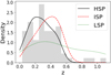 |
Fig. 6. Redshift distribution for the sources in the XMM–Newton BL Lac catalogue. Grey bars represent all BL Lacs for which the redshift is known (60% of the total sample), while curves represent the KDE curves for the subpopulations HSP (solid black), ISP (dashed red), and LSP (dotted green). |
In order to derive average X-ray spectral parameters from the best-fit model, we need to establish first which spectral model out of the six tested best fits the data on average (Sect. 3.3.6). Also, we need to remove any bias introduced by the existence of many observations from certain sources. In the coming sections, we discuss the selection of the best-spectral-fit model and then the average X-ray spectral properties derived from it.
5.2. Best-fit model
In order to determine which spectral model best fits the data, we use the fit results from the combination of the EPIC detectors, indicated as “epic” in column Inst of Table B.2, which are free or successfully corrected for pile-up. For every single observation, this can be any combination of one, two, or three EPIC cameras. This leaves a total of 218 observations, which are used to extract results for each one of the six available models.
The power law and log parabola models with the different flavours of NH are fitted uniformly to the entire sample. The goodness of fit is evaluated using χ2 statistics. Figure 7 presents a box plot of the distribution of  for the six models applied and described in Sect. 3.3.6. This type of plot is a non-parametric method for graphically representing variation in samples of a statistical population without making any assumptions as to the underlying statistical distribution. These plots show the median, the upper (Q3, 75%), and lower (Q1, 25%) quantiles, the minimum and maximum values after excluding possible outliers (indicated in the figure by the whiskers), the confidence interval (represented as 1.5× (Q3–Q1) and indicated in the figure by a notch), and outliers (indicated in the figure by the stars).
 |
Fig. 7.
|

Figure 7 shows that the best models in terms of goodness of fit are both the log parabola with NH free and the log parabola with two NH components (NH, Gal and NH, z). Of the six models tested, the log parabola with NH free provides the best fit in 71/218 cases, followed by the log parabola with two NH components (57/218). The power law model with two absorption components follows (35/218) and then the log parabola fixing NH (24/218). The power law with NH free (19/218) and fixing NH (12/218) provide the least number of times the best representation of the data. Figure 7 also shows that, on average, log parabola models provide a better fit to the data than power law models, with lower medians and less dispersion of  . A log parabola is favoured in 152/218 of the spectra fitted versus a simple power law which is favoured in 66/218. In terms of NH, using two NH components (NH, Gal and NH, z) provides better fits (92/218), while leaving the NH free to vary during the fitting procedure is favoured in 90/218 spectra and fixing NH to the NH, Gal is favoured in 36/218 spectra.
In Fig. 8 we represent the flux distributions in the 0.2–10.0 keV band for those sources for which the power law model is preferred and those best fitted by a log parabola (combining all three absorption flavours), and see that those sources favouring a log parabola present significantly higher fluxes. We use a t-test and reject the null hypothesis that the means of both distributions are equal considering different variances with 99% confidence. The fact that the log parabola is preferred for sources that show higher fluxes, that is, sources with higher S/N as in Donato et al. (2005), might indicate that curvature is intrinsic to this type of object but only shows when the S/N is sufficiently high.
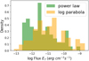 |
Fig. 8. Flux distribution in the band 0.2–10.0 keV (in green) for the sources best fitted by the power law model, and the same for the log parabola (in orange) combining all three absorption flavours. |
5.3. Spectral properties
For the following analysis, we only consider the best-fit model log parabola with NH free, and we exclude from this sample those ObsIds poorly fitted with a value for the  and those ObsIds that show pile-up in any of the EPIC cameras (see Table 1). After filtering, we have 200 ObsIds that correspond to 79 different BL Lacs. To avoid over-representation by sources observed multiple times we adopt the following procedure (Donato et al. 2005):
– For non-variable sources that only show small variations in both photon index and flux in the 0.2–10 keV band, that is, ΔΓ ≤ 0.5 and flux variation of a factor of less than two between maximum and minimum, we use the mean value for all output parameters derived using the log parabola with NH free model. Given that XSPEC returns asymmetric errors, the mean and its error are calculated as follows: for each of the 200 ObsIds, we create a Gaussian distribution centred at the parameter’s value and a total dispersion with an amplitude of the asymmetric error, and take a value inside this distribution. We repeat this process 1000 times and choose as the mean parameter the mean of all simulations for each BL Lac.
– For variable sources that show significant photon index and/or flux variations, that is, ΔΓ > 0.5 and/or flux variation of a factor of greater than two between maximum and minimum, we consider the observations corresponding to the extreme parameters, so that the source is represented in both states.
The result of this exercise is what we refer to as a non-biased sample and is summarised in the fourth table of the catalogue, named “multifreq” as explained in Sect. 4.1, and its columns are reported and described in Table B.4.
We study the model parameters separating them according to BL Lac subpopulations, seeing that the photon index is steepest for ISPs, followed by LSPs, and lastly HSPs (Γ = 2.84, 2.59 and 2.49, respectively, as seen in the top panel of Fig. 9). The ISP distribution is shifted towards higher ΓX values, however this effect might be affected by the source 5BZBJ0021−2550, for which ΓX = 3.99, although the model clearly does not represent the data well enough as  = 0.6124. As for the curvature parameter βX, LSPs are those showing the lowest values (distribution peaks at −0.289) while ISPs and HSPs show values for the peak of the distribution at −0.209 and −0.013 respectively, as seen in the bottom panel of Fig. 9. Only a few sources have positive βX values, which could indicate an upward curvature due to the presence of both synchrotron and inverse Compton components (Giommi et al. 2002).
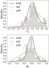 |
Fig. 9. Top: log parabola NH free model photon index ΓX distribution for the non-biased sample of BL Lacs (grey bars), and curves showing the KDE for the subpopulations HSP (black solid line), ISP (dashed red line), and LSP (green dotted line). Bottom: idem βX distribution. |
5.4. Luminosity
The distribution of the X-ray luminosity in the intervals 0.2–10.0 keV, 0.2–2.0 keV, and 2.0–10.0 keV for the non-biased sample is given in Fig. 10 in the top, middle, and bottom panels, respectively. The peak of the distribution for BL Lacs in the 0.2–10.0 keV band falls at  erg s−1. LSPs are the most luminous BL Lacs in X-rays, where the median values in the 0.2–10.0 keV band, are
  ,
,  9.58, and
  in units of 1044 erg s−1. This is true for both soft and hard bands.
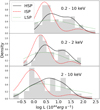 |
Fig. 10. Luminosity distribution of the non-biased sample in the energy intervals 0.2–10.0 keV (top), 0.2–2.0 keV (middle), and 2.0–10.0 (bottom). Grey bars represent sources with available redshift, while curves represent the KDE for HSPs (solid black), ISPs (dashed red), and LSPs (dotted green). |
5.5. Variability
The fraction of BL Lacs reported as variable in either band according to the χ2 probability of the constancy test is 56/103 (∼54%). These sources are mostly HSPs (31), but also there are 9 ISPs and 14 LSPs that are variable, and 5 of them remain unclassified. The peak of the synchrotron emission  for variable BL Lacs lies at higher values (
 ) than for non-variable BL Lacs (
 ). Additionally, most of the sources that are strong γ-ray emitters are variable (13/18 TeV sources and 42/63 4FGL sources).
6. Conclusions
This paper presents the XMM–Newton BL Lac catalogue, which comprises a sample of those BL Lacs reported by BZCAT observed with XMM–Newton over almost 20 years of the mission. We report results from a total of 310 observations that contain information on 103 different BL Lacs.
We have developed an analysis pipeline to automatically cross-match sources from the BZCAT catalogue and XMM–Newton public observations contained in the XSA archive as of September 2019. Source-matching and detection algorithms yield 310 positive X-ray source identifications which have been homogeneously analysed to generate XMM–Newton images, spectra, and light curves from the three EPIC cameras. OM exposures within these observations are also reduced when available and visual magnitudes and fluxes are provided.
While the sources contained in the XMM–Newton BL Lac catalogue are also present in the 4XMM, our pipeline has been specifically designed for the analysis of BL Lacs. The main difference can be found in the derivation of the reported fluxes. The pipeline used to extract the 4XMM is optimised for source detectability and to homogeneously account for all the different classes of sources included in the catalogue. Unlike in the XMM–Newton BL Lac catalogue, 4XMM sources are not pile-up corrected and the fluxes are derived from energy conversion factors (ECFs), assuming a spectral model of an absorbed power law with absorbing column density Nh = 3.0 × 1020 cm2 and continuum spectral slope Γ = 1.7 (Rosen et al. 2016).
We extracted close to 1000 background-subtracted light curves over two different energy ranges, soft and hard, together with time variability information following statistical indicators. Half of our sample shows indication for variable X-ray emission, most attributed to HSPs. Regarding the spectra, we performed around 7000 spectral fits to extract the best-fit model X-ray spectral parameters for two different models, namely power law and log parabola, with three different flavours for the absorption column density (fixed to the galactic column density, left free to vary, and a combination of galactic column density plus extra local absorption). We observe a wide span of photon indices, from the very flat hard values indicating inverse-Compton-dominated spectra up to very steep soft indices where the tail of the synchrotron emission reaches the X-rays. The curvature parameter is mostly negative and lower for sources with lower νpeak, reaching minimum values for LSPs.
As in previous works (Giommi et al. 2002; Donato et al. 2005; Perlman et al. 2005) we find that the model that best represents the X-ray spectra of BL Lacs is the log parabola with NH left free to vary. Moreover, we see that models best fit by a log parabola show higher fluxes than those best represented by a power law, indicating that curvature is intrinsic to this type of object; however we are only able to evaluate curvature when spectra have high S/N. Massaro et al. (2004) explained the log parabolic spectrum as the result of a statistical acceleration mechanism in which the probability of a particle to remain inside an acceleration region decreases as the energy of the particles increases.
The XMM–Newton BL Lac catalogue is intended to be used as a valuable resource to better understand BL Lacs in the X-rays and their correlations with other wavelengths. Incremental releases are planned to augment this catalogue, with continuous efforts made by the astronomical community in discovering new BL Lacs and more observations becoming available in the XMM–Newton archive in coming years. XMM–Newton instruments remain in good health and are expected to continue being operational for several more years.
Acknowledgments
We thank the anonymous referee for her/his insightful comments that led to significant improvements in the paper. IC would like to thank the XMM–Newton SOC and its members for many fruitful discussions. IC would like to acknowledge support by the Torres Quevedo fellowship programme from the Ministerio de Educación y Ciencia Español and from INSA, and to N. Loiseau who proposed this fellowship. NAC is supported by European Space Agency (ESA) Research Fellowships. This work is based on observations with XMM–Newton, an ESA science mission with instruments and contributions directly funded by ESA Member States and NASA. This research has made use of data archives, catalogues and software tools from the ASDC, a facility managed by the Italian Space Agency (ASI). This research has made use of the NASA/IPAC Extragalactic Database, operated by the Jet Propulsion Laboratory, Caltech, under the contract with NASA, and the NASA Astrophysics Data System Abstract Service.
References
- Abdo, A. A., Ackermann, M., Ajello, M., et al. 2010a, ApJS, 188, 405 [NASA ADS] [CrossRef] [Google Scholar]
- Abdo, A. A., Ackermann, M., Agudo, I., et al. 2010b, ApJ, 716, 30 [NASA ADS] [CrossRef] [Google Scholar]
- Abdollahi, S., Acero, F., Ackermann, M., et al. 2020, ApJs, 247, 33 [NASA ADS] [CrossRef] [Google Scholar]
- Acciari, V. A., Aliu, E., Beilicke, M., et al. 2008, ApJ, 684, L73 [NASA ADS] [CrossRef] [Google Scholar]
- Acero, F., Ackermann, M., Ajello, M., et al. 2015, ApJS, 218, 23 [Google Scholar]
- Ackermann, M., Ajello, M., Atwood, W. B., et al. 2015, ApJ, 810, 14 [NASA ADS] [CrossRef] [Google Scholar]
- Agudo, I., Krichbaum, T. P., Ungerechts, H., et al. 2006, A&A, 456, 117 [NASA ADS] [CrossRef] [EDP Sciences] [Google Scholar]
- Aharonian, F. A. 2000, New Astron., 5, 377 [NASA ADS] [CrossRef] [Google Scholar]
- Aharonian, F., Akhperjanian, A. G., Bazer-Bachi, A. R., et al. 2006, A&A, 455, 461 [NASA ADS] [CrossRef] [EDP Sciences] [Google Scholar]
- Ahn, C. P., Alexandroff, R., Allende Prieto, C., et al. 2012, ApJS, 203, 21 [Google Scholar]
- Ajello, M., Angioni, R., Axelsson, M., et al. 2020, ApJ, 892, 105 [NASA ADS] [CrossRef] [Google Scholar]
- Álvarez Crespo, N., Massaro, F., Milisavljevic, D., et al. 2016, AJ, 151, 95 [CrossRef] [Google Scholar]
- Arnaud, K. A. 1996, in Astronomical Data Analysis Software and Systems V, eds. G. H. Jacoby, & J. Barnes, ASP Conf. Ser., 101, 17 [NASA ADS] [Google Scholar]
- Bach, U., Krichbaum, T. P., Kraus, A., Witzel, A., & Zensus, J. A. 2006, A&A, 452, 83 [NASA ADS] [CrossRef] [EDP Sciences] [Google Scholar]
- Blandford, R. D., & Rees, M. J. 1978, Phys. Scr., 17, 265 [CrossRef] [Google Scholar]
- Brinkmann, W., Papadakis, I. E., Raeth, C., Mimica, P., & Haberl, F. 2005, A&A, 443, 397 [NASA ADS] [CrossRef] [EDP Sciences] [Google Scholar]
- Condon, J. J., Cotton, W. D., Greisen, E. W., et al. 1998, AJ, 115, 1693 [Google Scholar]
- D’Abrusco, R., Massaro, F., Ajello, M., et al. 2012, ApJ, 748, 68 [CrossRef] [Google Scholar]
- D’Abrusco, R., Massaro, F., Paggi, A., et al. 2014, ApJS, 215, 14 [Google Scholar]
- D’Abrusco, R., Álvarez Crespo, N., Massaro, F., et al. 2019, ApJS, 242, 4 [Google Scholar]
- de Menezes, R., D’Abrusco, R., Massaro, F., Gasparrini, D., & Nemmen, R. 2020, ApJS, 248, 23 [NASA ADS] [CrossRef] [Google Scholar]
- Deng, X.-C., Hu, W., Lu, F.-W., & Dai, B.-Z. 2021, MNRAS, 504, 878 [CrossRef] [Google Scholar]
- Donato, D., Sambruna, R. M., & Gliozzi, M. 2005, A&A, 433, 1163 [NASA ADS] [CrossRef] [EDP Sciences] [Google Scholar]
- Falcone, A. D., Cui, W., & Finley, J. P. 2004, ApJ, 601, 165 [NASA ADS] [CrossRef] [Google Scholar]
- Fossati, G., Maraschi, L., Celotti, A., Comastri, A., & Ghisellini, G. 1998, MNRAS, 299, 433 [Google Scholar]
- Gabriel, C., Denby, M., Fyfe, D. J., et al. 2004, in The XMM-Newton SAS - Distributed Development and Maintenance of a Large Science Analysis System: A Critical Analysis, eds. F. Ochsenbein, M. G. Allen, & D. Egret, ASP Conf. Ser., 314, 759 [Google Scholar]
- Galbiati, E., Caccianiga, A., Maccacaro, T., et al. 2005, A&A, 430, 927 [NASA ADS] [CrossRef] [EDP Sciences] [Google Scholar]
- Ghisellini, G. 1999, Astropart. Phys., 11, 11 [NASA ADS] [CrossRef] [Google Scholar]
- Ghisellini, G., Celotti, A., George, I. M., & Fabian, A. C. 1992, MNRAS, 258, 776 [NASA ADS] [CrossRef] [Google Scholar]
- Ghisellini, G., Celotti, A., Fossati, G., Maraschi, L., & Comastri, A. 1998, MNRAS, 301, 451 [NASA ADS] [CrossRef] [Google Scholar]
- Ghisellini, G., Righi, C., Costamante, L., & Tavecchio, F. 2017, MNRAS, 469, 255 [NASA ADS] [CrossRef] [Google Scholar]
- Giommi, P., Capalbi, M., Fiocchi, M., et al. 2002, Blazar Astrophysics with BeppoSAX and Other Observatories, eds. P. Giommi, E. Massaro, & G. Palumbo, 63 [Google Scholar]
- Giommi, P., Padovani, P., Polenta, G., et al. 2012, MNRAS, 420, 2899 [NASA ADS] [CrossRef] [Google Scholar]
- H.E.S.S. Collaboration (Abramowski, A., et al.) 2010, A&A, 516, A56 [CrossRef] [EDP Sciences] [Google Scholar]
- H.E.S.S. Collaboration (Abramowski, A., et al.) 2014, A&A, 564, A9 [NASA ADS] [CrossRef] [EDP Sciences] [Google Scholar]
- HI4PI Collaboration (Ben Bekhti, N., et al.) 2016, A&A, 594, A116 [NASA ADS] [CrossRef] [EDP Sciences] [Google Scholar]
- Jansen, F., Lumb, D., Altieri, B., et al. 2001, A&A, 365, L1 [NASA ADS] [CrossRef] [EDP Sciences] [Google Scholar]
- Jethwa, P., Saxton, R., Guainazzi, M., Rodriguez- Pascual, P., & Stuhlinger, M. 2015, A&A, 581, A104 [NASA ADS] [CrossRef] [EDP Sciences] [Google Scholar]
- Kapanadze, B. Z. 2009, MNRAS, 398, 832 [NASA ADS] [CrossRef] [Google Scholar]
- Kapanadze, B. Z. 2013, AJ, 145, 31 [NASA ADS] [CrossRef] [Google Scholar]
- Kushwaha, P., & Pal, M. 2020, Galaxies, 8, 66 [NASA ADS] [CrossRef] [Google Scholar]
- Lico, R., Giroletti, M., Orienti, M., & D’Ammando, F. 2016, A&A, 594, A60 [NASA ADS] [CrossRef] [EDP Sciences] [Google Scholar]
- Lumb, D. H., Warwick, R. S., Page, M., & De Luca, A. 2002, A&A, 389, 93 [NASA ADS] [CrossRef] [EDP Sciences] [Google Scholar]
- Mannheim, K. 1996, Space Sci. Rev., 75, 331 [NASA ADS] [CrossRef] [Google Scholar]
- Mason, K. O., Breeveld, A., Much, R., et al. 2001, A&A, 365, L36 [NASA ADS] [CrossRef] [EDP Sciences] [Google Scholar]
- Massaro, E., Perri, M., Giommi, P., & Nesci, R. 2004, A&A, 413, 489 [NASA ADS] [CrossRef] [EDP Sciences] [Google Scholar]
- Massaro, F., D’Abrusco, R., Ajello, M., Grindlay, J. E., & Smith, H. A. 2011, ApJ, 740, L48 [NASA ADS] [CrossRef] [Google Scholar]
- Massaro, E., Maselli, A., Leto, C., et al. 2015, Astrophys. Space Sci., 357, 75 [NASA ADS] [CrossRef] [Google Scholar]
- Mateos, S., Saxton, R. D., Read, A. M., & Sembay, S. 2009, A&A, 496, 879 [NASA ADS] [CrossRef] [EDP Sciences] [Google Scholar]
- Mauch, T., Murphy, T., Buttery, H. J., et al. 2003, MNRAS, 342, 1117 [Google Scholar]
- Monet, D. G., Levine, S. E., Canzian, B., et al. 2003, AJ, 125, 984 [Google Scholar]
- Morrison, R., & McCammon, D. 1983, ApJ, 270, 119 [Google Scholar]
- Mücke, A., Protheroe, R. J., Engel, R., Rachen, J. P., & Stanev, T. 2003, Astropart. Phys., 18, 593 [Google Scholar]
- Nandra, K., George, I. M., Mushotzky, R. F., Turner, T. J., & Yaqoob, T. 1997, ApJ, 476, 70 [Google Scholar]
- Nolan, P. L., Abdo, A. A., Ackermann, M., et al. 2012, ApJS, 199, 31 [Google Scholar]
- Oke, J. B. 1974, ApJs, 27, 21 [NASA ADS] [CrossRef] [Google Scholar]
- Our, A. C. 1969, Nature, 223, 566 [Google Scholar]
- Padovani, P., & Giommi, P. 1995, ApJ, 444, 567 [NASA ADS] [CrossRef] [Google Scholar]
- Page, M. J., Brindle, C., Talavera, A., et al. 2012, MNRAS, 426, 903 [NASA ADS] [CrossRef] [Google Scholar]
- Perlman, E. S., Madejski, G., Georganopoulos, M., et al. 2005, ApJ, 625, 727 [NASA ADS] [CrossRef] [Google Scholar]
- Pian, E., Romano, P., Treves, A., et al. 2007, ApJ, 664, 106 [NASA ADS] [CrossRef] [Google Scholar]
- Pigg, J. C., & Cohen, M. H. 1971, PASP, 83, 680 [NASA ADS] [CrossRef] [Google Scholar]
- Rosen, S. 2020, XMM-Newton Optical and UV Monitor (OM) Calibration Status http://xmmweb.esac.esa.int/docs/documents/CAL-TN-0019.pdf [Google Scholar]
- Rosen, S. R., Webb, N. A., Watson, M. G., et al. 2016, A&A, 590, A1 [NASA ADS] [CrossRef] [EDP Sciences] [Google Scholar]
- Sahu, S., López Fortín, C. E., Castañeda Hernández, L. H., Nagataki, S., & Rajpoot, S. 2020, ApJ, 901, 132 [NASA ADS] [CrossRef] [Google Scholar]
- Schmitt, J. L. 1968, Nature, 218, 663 [NASA ADS] [CrossRef] [Google Scholar]
- Sikora, M., & Madejski, G. 2001, AIP Conf. Ser., 558, 275 [NASA ADS] [CrossRef] [Google Scholar]
- Skrutskie, M. F., Cutri, R. M., Stiening, R., et al. 2006, AJ, 131, 1163 [NASA ADS] [CrossRef] [Google Scholar]
- Smith, M. 2019, EPIC Status of Calibration and Data Analysis, http://xmmweb.esac.esa.int/docs/documents/CAL-TN-0018.pdf [Google Scholar]
- Smith, M. 2020, Routine Calibration Plan, http://xmmweb.esac.esa.int/docs/documents/CAL-PL-0001.pdf [Google Scholar]
- Stickel, M., Padovani, P., Urry, C. M., Fried, J. W., & Kuehr, H. 1991, ApJ, 374, 431 [Google Scholar]
- Strüder, L., Briel, U., Dennerl, K., et al. 2001, A&A, 365, L18 [Google Scholar]
- Turner, M. J. L., Abbey, A., Arnaud, M., et al. 2001, A&A, 365, L27 [CrossRef] [EDP Sciences] [Google Scholar]
- Urry, C. M., & Padovani, P. 1995, PASP, 107, 803 [NASA ADS] [CrossRef] [Google Scholar]
- Vaughan, S., Edelson, R., Warwick, R. S., & Uttley, P. 2003, MNRAS, 345, 1271 [Google Scholar]
- Webb, N. A., Coriat, M., Traulsen, I., et al. 2020, A&A, 641, A136 [NASA ADS] [CrossRef] [EDP Sciences] [Google Scholar]
- Wu, Z., Jiang, D. R., Gu, M., & Liu, Y. 2007, A&A, 466, 63 [NASA ADS] [CrossRef] [EDP Sciences] [Google Scholar]
- Zhang, Y. H., Bai, J. M., Zhang, S. N., et al. 2006, ApJ, 651, 782 [NASA ADS] [CrossRef] [Google Scholar]
Appendix A: Appendix A: Sources with long cumulative exposure times.
Nineteen BL Lacs in our catalogue have long cumulative exposure times of over 100 ks, as a result of the existence of several observations, in some cases, spread out over several years. Amongst these BL Lacs, eight are serendipitous sources contained in the FOV of XMM–Newton target observations. Most of these eight sources are contained in different samples of objects selected according to different properties. Below we summarise some of their X-ray spectral properties.
5BZBJ0057-2212. Of unknown redshift, there are four observations contained in the catalogue (2000, 2002, 2015 and 2016). All observations but one show a weak X-ray source for which it is not possible to extract good-quality spectra. For the observation with best statistics (2015), the optimal fit is provided by a power law model with two absorption components. The photon index is 1.84 with a flux of 3.24 ⋅ 10−13 erg cm−2 s−1 in the 0.2 - 10 keV range. The source shows no sign of variability within the timescale of the observations for the default 500 s bins used.
5BZBJ0333-3619. This BL Lac is observed at z= 0.308. Twelve observations spanning 2003 - 2013 are included in the catalogue and all but one are best fitted by a log parabolic model. The average flux is about 0.5 − 3.5 ⋅ 10−12 erg cm−2 s−1 in the 0.2 - 10 keV range. This source is part of a sample of AGNs that have been the target of TeV observations by H.E.S.S. up to 2011 that show no significant excess in high-energy emission (H.E.S.S. Collaboration 2014). There is no significant variability within the timescale of the observations for the default 500 s bins used.
5BZBJ0613+7107. The redshift of this source is 0.267. Sixteen observations from 2000 to 2015 are contained in the catalogue. Eight observations show a weak X-ray source for which it is not possible to extract good-quality spectra. For the remaining observations, the most favoured fit is provided by a power law model with two absorption components, although in several observations a log parabolic model fits better. The flux ranges between 0.6 − 1.3 ⋅ 10−12 erg cm−2 s−1 in the 0.2 - 10 keVrange. There is no significant variability within the timescale of the observations for the default 500 s bins used.
5BZBJ0721+7120. (also known as PKS 0716+714) has been extensively studied because of its intraday variability. Simultaneous radio, optical, UV, and X-ray observations yielded a short duty cycle of variability at all frequencies and a correlation between different wavelengths (Agudo et al. 2006). VLBI images show a compact, one-sided core jet (Bach et al. 2006). Of unknown redshift, five observations are found between 2001 and 2007 in our catalogue. In the 2001 and 2002 observations, this is a field source while in 2004 and 2007 it was the XMM–Newton target, part of a target of opportunity (ToO) program to explore blazars in outburst. During 2004 and 2007 the source displayed high flux variability within the XMM–Newton observations, with rapid flares of the order of a few hours (Kushwaha & Pal 2020). During these observations the average flux was of the order of 1.0 ⋅ 10−11 erg cm−2 s−1 in the 0.2 - 10 keV range. In all observations the best fit is provided by a log parabolic model.
5BZBJ0958+6533. This is a LSP BL Lac at z= 0.367 and famous for its intraday variability (Bach et al. 2006). It shows a one-sided jet structure that bends from milliarcsecond to arcsecond scales (Lico et al. 2016). There are three observations contained in our catalogue, one from 2005 and two from 2007. In all cases, the log parabolic model provides the best fit. The X-ray flux in the 0.2 - 10 keV range varies between 2.5 and 3.3⋅10−13 erg cm−2 s−1. The first observation in 2007 shows a significant steady increase, a factor two, in flux over the course of the observation, more noticeable in the low 0.2-2.0 keV energy range, which results in a softening of the spectrum over the course of the observation.
5BZBJ1136+1601. This BL Lac lies at z= 0.574. There are five observations contained in our catalogue taken between May and June 2014. In all cases, the best-fit model is a power law with two absorption components and photon index between 2.4 and 2.8. The X-ray flux in the 0.2 - 10 keV range varies between 2.2 and 2.5⋅10−13 erg cm−2 s−1. There is no significant variability within the timescale of the observations for the default 500 s bins used.
5BZBJ1210+3929. The redshift of this source is z= 0.617. We report nine observations in total from 2000 (2x), 2011 (3x), and 2012 (4x). All observations are best fitted by a power law with two absorption components. The photon index varies between 2.1 and 2.3 and the X-ray flux varies in the range 3.0 − 8.2 ⋅ 10−12 erg cm−2 s−1 in the 0.2 - 10 keV range. The source does not display significant source variability, being consistent with a constant source over the course of the observations.
5BZBJ2258-3644. Of unknown redshift, two observations are present in the catalogue, from 2005 and 2015. In both cases the spectra are best fitted by a power law with two absorption components. The photon index of the 2005 observation is 2.9 and the flux 3.67 ⋅ 10−13 erg cm−2 s−1 in the 0.2 - 10 keV range; while in the 2015 the photon index is 3.33 and the flux 4.96 ⋅ 10−13 erg cm−2 s−1 in the 0.2 - 10 keV range.
All Tables
53 observations with at least one EPIC exposure where pile-up is present and cannot be corrected.
XMM–Newton observations where no X-ray emission is detected at the location of the BZCAT source.
All Figures
|
Fig. 1. Equatorial coordinates of the BL Lacs from BZCAT, indicated as black points. Red crosses mark the distribution of those sources contained in the catalogue of XMM–Newton BL Lacs. |
| In the text | |
|
Fig. 2. Distribution of the exposure time (in ks) of single observations included in the catalogue of XMM–Newton BL Lacs. |
| In the text | |
|
Fig. 3. Top: EPIC IMAGING Full Frame mode source (orange) and background (red) extraction region definition for the source 5BZBJ0333-3619. Left panel: PN, middle panel: MOS1, and right panel: MOS2 cameras. Bottom: EPIC IMAGING Small Window mode source (orange) and background (red) extraction region definition for the source 5BZBJ0326+0225. |
| In the text | |
|
Fig. 4. EPIC IMAGING mode thumbnail true colour images around the X-ray source 5BZBJ0613+7107 marked by a red cross (Events in red: 0.5–4.5 keV, green: 4.5–7.5 keV, blue: 7.5–12.0 keV). Blue circles mark other X-ray sources in the field. |
| In the text | |
|
Fig. 5. Example light curve and spectra of 5BZBJ1221+2813. Left: EPIC-pn light curve in the 0.2–2.0 keV (top) and 2.0–10.0 keV (middle) bands and hardness ratio (bottom). Red symbols indicate those bins for which the effective exposure is below 15%. Right: combined spectral fit for EPIC-pn (black), EPIC-MOS1 (green), and EPIC-MOS2 (red) spectra corresponding to the power law with the two-absorption-component model. |
| In the text | |
|
Fig. 6. Redshift distribution for the sources in the XMM–Newton BL Lac catalogue. Grey bars represent all BL Lacs for which the redshift is known (60% of the total sample), while curves represent the KDE curves for the subpopulations HSP (solid black), ISP (dashed red), and LSP (dotted green). |
| In the text | |
|
Fig. 7.
|
| In the text | |
|
Fig. 8. Flux distribution in the band 0.2–10.0 keV (in green) for the sources best fitted by the power law model, and the same for the log parabola (in orange) combining all three absorption flavours. |
| In the text | |
|
Fig. 9. Top: log parabola NH free model photon index ΓX distribution for the non-biased sample of BL Lacs (grey bars), and curves showing the KDE for the subpopulations HSP (black solid line), ISP (dashed red line), and LSP (green dotted line). Bottom: idem βX distribution. |
| In the text | |
|
Fig. 10. Luminosity distribution of the non-biased sample in the energy intervals 0.2–10.0 keV (top), 0.2–2.0 keV (middle), and 2.0–10.0 (bottom). Grey bars represent sources with available redshift, while curves represent the KDE for HSPs (solid black), ISPs (dashed red), and LSPs (dotted green). |
| In the text | |
Current usage metrics show cumulative count of Article Views (full-text article views including HTML views, PDF and ePub downloads, according to the available data) and Abstracts Views on Vision4Press platform.
Data correspond to usage on the plateform after 2015. The current usage metrics is available 48-96 hours after online publication and is updated daily on week days.
Initial download of the metrics may take a while.