| Issue |
A&A
Volume 654, October 2021
|
|
|---|---|---|
| Article Number | A93 | |
| Number of page(s) | 12 | |
| Section | Extragalactic astronomy | |
| DOI | https://doi.org/10.1051/0004-6361/202141797 | |
| Published online | 18 October 2021 | |
Polar dust obscuration in broad-line active galaxies from the XMM-XXL field⋆
1
Aix Marseille Univ, CNRS, CNES, LAM, Marseille, France
e-mail: This email address is being protected from spambots. You need JavaScript enabled to view it.
2
Institut Universitaire de France (IUF), Paris, France
3
Instituto de Fisica de Cantabria (CSIC-Universidad de Cantabria), Avenida de los Castros, 39005 Santander, Spain
4
Department of Physics and Astronomy, Texas A&M University, College Station, TX 77843-4242, USA
5
George P. and Cynthia Woods Mitchell Institute for Fundamental Physics and Astronomy, Texas A& M University, College Station, TX 77843-4242, USA
6
Centro de Astronomía (CITEVA), Universidad de Antofagasta, Avenida Angamos 601, Antofagasta, Chile
7
Astronomical Observatory, Volgina 7, 11060 Belgrade, Serbia
8
Sterrenkundig Observatorium, Universiteit Ghent, Krijgslaan 281- S9, Ghent 9000, Belgium
Received:
15
July
2021
Accepted:
3
August
2021
Abstract
Aims. Dust is observed in the polar regions of nearby active galactic nuclei (AGN) and it is known to contribute substantially to their mid-IR emission and to the obscuration of their UV to optical emission. We aim to carry out a statistical test to check whether this component is a common feature based on an analysis of the integrated spectral energy distributions of these composite sources.
Methods. We selected a sample of 1275 broad-line AGN in the XMM-XXL field, with optical to infrared photometric data. These AGN are seen along their polar direction and we expect a maximal impact of dust located around the poles when it is present. We used X-CIGALE, which introduces a dust component to account for obscuration along the polar directions, modeled as a foreground screen, and an extinction curve that is chosen as it steepens significantly at short wavelengths or is much grayer. By comparing the results of different fits, we are able to define subsamples of sources with positive statistical evidence in favor of or against polar obscuration (if present) and described using the gray or steep extinction curve.
Results. We find a similar fraction of sources with positive evidence for and against polar dust. Applying statistical corrections, we estimate that half of our sample could contain polar dust and among them, 60% exhibit a steep extinction curve and 40% a flat extinction curve; although these latter percentages are found to depend on the adopted extinction curves. The obscuration in the V-band is not found to correlate with the X-ray column density, while AV/NH ratios span a large range of values and higher dust temperatures are found with the flat, rather than with the steep extinction curve. Ignoring this polar dust component in the fit of the spectral energy distribution of these composite systems leads to an overestimation of the stellar contribution. A single fit with a polar dust component described with an SMC extinction curve efficiently overcomes this issue but it fails at identifying all the AGN with polar dust obscuration.
Key words: galaxies: active / galaxies: nuclei / dust, extinction / methods: data analysis
Full Table A.1 is only available at the CDS via anonymous ftp to cdsarc.u-strasbg.fr (130.79.128.5) or via http://cdsarc.u-strasbg.fr/viz-bin/cat/J/A+A/654/A93
© V. Buat et al. 2021
 Open Access article, published by EDP Sciences, under the terms of the Creative Commons Attribution License (https://creativecommons.org/licenses/by/4.0), which permits unrestricted use, distribution, and reproduction in any medium, provided the original work is properly cited.
1. Introduction
Modeling the characteristics of dust obscuration is crucial in determining the intrinsic spectral energy distribution (SED) of any astronomical source from the ultraviolet (UV) to the near-infrared (near-IR). It is especially crucial for quasars and active galactic nuclei (AGN) that are strong UV emitters: even a small amount of dust can reshape dramatically their SED. The spectral emission of AGN and quasars are found remarkably similar in the mid-infrared (mid-IR, e.g., Richards et al. 2006; Elvis et al. 2012; Assef et al. 2010). The primary difference between type 1 and type 2 AGN and quasar emission appears in the UV-optical regime and is attributed to dust reddening (e.g., Hickox et al. 2017). On the one hand, the UV to near-IR emission of type 2 sources is dominated by the host component and obscured active sources are mostly identified in the mid-IR (e.g., Stern et al. 2005; Donley et al. 2012; Assef et al. 2010). On the other hand, a large diversity of optical to near-IR SEDs is found for AGN type 1 sources and the departure to an unobscured type 1 SED, such as that of Elvis et al. (1994) is interpreted by dust obscuration or host galaxy contamination (Carleton et al. 1987; Richards et al. 2003; Prieto et al. 2010; Elvis et al. 2012; Hao et al. 2013; Yang et al. 2020).
The unification model (Antonucci 1993; Urry & Padovani 1995) introduces a central dusty torus and is very successful at explaining both the bulk of mid- and far-IR emissions and the broad and narrow emission lines observed in type 1 and type 2 sources. While this model is very efficient at explaining the main differences between AGN types by the orientation of the line of sight with respect to the dusty torus, more complex dust configurations have also been proposed from parsec scales (torus) to larger scales in the host galaxy (e.g., Netzer 2015; Chen et al. 2015; Asmus 2019; Zou et al. 2019).
Characterizing the nature of dust responsible of the obscuration of AGN is very difficult and different studies have led to diverse results. For instance, Richards et al. (2003) and Hopkins et al. (2004) found that an SMC extinction curve gives the best fits of SEDs of quasars from SDSS and this law is commonly used to redden the intrinsic emission of an AGN (e.g., Hao et al. 2013; Calistro Rivera et al. 2021). Conversely, Maiolino et al. (2001b) found observational evidence for different dust properties in moderately obscured local AGN than in the Galactic interstellar medium. They attributed these peculiar dust properties to a prominence of large grains, making the extinction curve flatter. Gaskell et al. (2004) derived extinction curves by comparing UV-optical composite continuum spectra and found a significantly flatter (i.e., grayer) curve with no rise in the UV, which is contrary to the SMC extinction law. Czerny et al. (2004) also derived an extinction curve flatter than the SMC law by comparing blue and red composite spectra of quasars from the SDSS. These flatter curves can be explained with modifications of the standard dust models with a deficit of small grains (Gaskell et al. 2004) or to a high rate of grain coagulation in a dense medium (Laor & Draine 1993; Maiolino et al. 2001a).
Thanks to mid-IR interferometry, some nearby AGN can now be observed at parsec scales and warm dust is commonly found distributed along the AGN polar direction (e.g., Asmus et al. 2016; López-Gonzaga et al. 2016). The polar dust extension may originate from dusty winds driven by the emission of the accretion disk. Its emission represents a substantial fraction of the mid-IR emission coming from the AGN (Asmus et al. 2016). Its distribution measured on mid-IR images is variable from tens to hundreds parsecs; Fuller et al. (2019) report even larger scales up to one kiloparsec. Stalevski et al. (2017, 2019) proposed a model to explain their high angular resolution mid-IR observations of the Circinus galaxy with a parsec scale optically thick disk and an optically thin dusty cone extending out to 40 parsecs. NGC 3783 can also be considered as a prototype of a type 1 source with a polar dust at a parsec scale composed of optically thick clouds and large carbon grains because of the selective destruction of silicate and small grains (Hönig & Kishimoto 2017; Lyu & Rieke 2018).
Various dusty structures can thus contribute to the obscuration of the nucleus emission: in addition to the equatorial dusty torus, which only affects type 2 AGN, some extra dust distributed around the polar direction can also redden the UV-optical emission of the accretion disk and contributes to the dust emission at IR wavelengths. The introduction of polar dust in the modeling of active galaxies of both types is found to impact the measure of parameters linked to dust, such as the covering factor of obscuring material (Asmus 2019; Toba et al. 2021) or the fraction of dust emission coming from the AGN (Mountrichas et al. 2021b). The identification of these multiple components and their relative contribution is difficult when only integrated multi-wavelength data are available, leading to degeneracies (e.g., Netzer 2015; Hao et al. 2013). Despite the complex distribution of dust around an AGN, simplified models must be used to investigate their main features (Lyu & Rieke 2018).
We present a study of a sample of X-ray selected type 1 sources spectroscopically identified with broad emission lines (BLAGN) in the XMM-XXL field (Pierre et al. 2016), and with a multi-wavelength coverage (Menzel et al. 2016). The impact of a potential polar dust component should be easier to measure in type 1 sources. According to the unification model, the nucleus emission is expected to emerge from the polar direction of these objects and we assume that any reddening of the AGN emission comes from the polar dust. Consequently, we merge the possible large-scale effect of the interstellar medium of the host with the reddening of a polar dust component since we are unable to disentangle both components from the integrated SEDs of the sources. For this study, we use the X-CIGALE code1 that accounts for polar dust modeled as a simple dust screen in front of the accretion disk and a dust extinction curve. We aim to test the presence of polar dust and to characterize its extinction curve. We also study the impact of this component to the measure of physical parameters related to host galaxy and AGN components.
In Sect. 2, we describe our composite models (AGN and host galaxy) created with X-CIGALE to fit the SEDs of our sources and using optical-IR colors, we highlight the impact on the optical-IR emission of dust reddening with either a steep (SMC, Pei 1992) or a gray (Gaskell et al. 2004, hereafter, G04) extinction curve. In Sect. 3, the SEDs of our sample of BLAGN in the XMM-XXL field are fitted with the different models presented in Sect. 2. We define sub-samples of sources described without any obscuration or with a polar dust and a given extinction curve in Sect. 3. We discuss our estimations of polar dust extinction and temperature. The properties of the host are compared in Sect. 4 for the sub-populations with and without polar dust, and the impact of the polar dust component on the determination of these properties is discussed in Sect. 5, while Sect. 6 is dedicated to a summary of our study. In this paper we assume a ΛCDM cosmology with parameters coming from the seven-year data from WMAP (Komatsu et al. 2011).
2. X-CIGALE modeling
CIGALE (Noll et al. 2009; Boquien et al. 2019), along with its X-ray extension X-CIGALE (Yang et al. 2020), is a very versatile code aimed at generating spectral models to fit the observed SEDs of extragalactic systems. It combines a stellar SED with a dust component emitting in the IR and conserves the energy balance between dust absorbed emission and its thermal re-emission. An AGN component can be added with its emission also modeled on the basis of the conservation of energy. The relative contribution of the AGN, fAGN, is measured as the fraction of total dust luminosity coming from the dusty torus and dust in polar regions (if present). Recently, Yang et al. (2020) developed a new branch of CIGALE, named X-CIGALE, with a phenomenological modeling of the X-ray emission to account for X-ray fluxes in the fits of the SED. It is this version of the code that we use in this work.
2.1. AGN component
Yang et al. (2020) implemented a clumpy two-phase torus model, SKIRTOR (Stalevski et al. 2012, 2016), based on the radiation transfer code, SKIRT (Baes & Camps 2015). To account for the possible presence of dust in the polar regions that is not included in SKIRTOR, a new component called “polar dust” is added to the SKIRTOR model as a homogeneous dust screen in the foreground of the accretion disk characterized by different extinction curves. Energy conservation is also applied to this new component, and the re-emission of dust in the polar regions is modeled as a modified black body. In this work, we use these new developments to model a BLAGN sample and we test the need to introduce any polar dust contribution. With our sample being X-ray selected, we ran X-CIGALE to fit simultaneously X-ray and UV to IR data. We considered models with and without an extra polar dust component described with either the SMC extinction curve of Pei (1992) or the flatter law of G04, both implemented in X-CIGALE. The shapes of these two curves allow us to investigate the role of polar dust in two very different contexts (Fig. 2 of Lyu et al. 2014, for a comparison of extinction laws). The G04 law expressed in Aλ/AV is essentially flat at wavelengths lower than the V-band (Fig. 3 of G04) and similar to the SMC and Milky Way extinction laws at longer wavelengths. Conversely, the SMC law increases steeply from the visible to shorter wavelengths; RV (defined as RV = AV/E(B − V)) values of both curves also reflect their differences with RV = 2.9 for SMC (Pei 1992) and RV = 5.5 for the analytical formula of the G04 curve implemented into X-CIGALE.
To illustrate the impact of the choice of the extinction law, in Fig. 1, we show the SED of the AGN component without polar dust and with a polar dust extinction calculated with either an SMC or a G04 law. The modification of the disk emission is clearly visible at rest-frame wavelengths lower than 0.5 μm. With the SMC law the intensity of the disk emission decreases sharply with wavelength, whereas it keeps its original shape when the G04 law is applied.
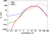 |
Fig. 1. SED of the AGN component modeled as described in Sect. 2.2. The scale of the fluxes is arbitrary. The red lines correspond to a polar dust obscuration of the accretion disk emission with an SMC extinction curve, the dust emission is the sum of torus and polar dust emission at 500 K (red solid line) and 100 K (dashed line). The green line corresponds to a polar dust obscuration with a G04 extinction curve. All models are normalized to the same energy emitted by dust. The SED of the model without polar dust is shown as a blue short-dashed line, in this case the dust emission comes only from the dusty torus and the emission of accretion disk is unabsorbed along the line of sight. |
We choose to compare SMC and G04 extinction curves as a first attempt to discriminate between two very different shapes of the AGN SEDs. The G04 curve was obtained for radio-loud AGN and is flatter than the extinction curve derived by Czerny et al. (2004) with composite spectra of red quasars from the Sloan Digital Sky Survey (SDSS). From their study of individual AGN, Gaskell & Benker (2007) found a large diversity of extinction curves and derived an average extinction curve that is not as flat as the G04 curve. In order to test the impact of the adopted extinction curves, we also considered the average extinction law of Gaskell & Benker (2007) in our analysis.
2.2. Composite models, AGN, and host galaxy
To highlight the effect of the polar dust component, we consider all our composite models built with X-CIGALE prior to the fitting process. They are composed of an AGN type 1 template and of a stellar component.
We use a delayed star formation history (SFH) with the functional form SFR ∝ texp(−t/τmain) for the star formation rate (SFR) of the main stellar population. A recent constant burst of star formation is over-imposed whose amplitude is measured by the stellar mass fraction produced during the burst, fburst (e.g., Buat et al. 2018). The ages of the two stellar populations are flexible. We adopt the Initial Mass Function of Chabrier (2003) and the stellar models of Bruzual & Charlot (2003) with a metallicity fixed to the solar value. The stellar emission is attenuated with the law of Calzetti et al. (2000), and the absorbed energy is re-emitted using Dale et al. (2014)2 templates parametrized by a single parameter α representing the relative contribution of different local heating conditions.
Following Yang et al. (2020), the AGN type 1 component is modeled by fixing the viewing angle to 30 degrees. All the other fixed input parameters describing the torus model of SKIRTOR are fixed as in Yang et al. (2020, their Table 2). We use the disk continuum emission from SKIRTOR with four power-laws to cover the full range from 0.008 μm to 1000 μm. In a new version of X-CIGALE, Yang et al. (in prep.) introduce a flexible power-law indice for 0.1 < λ < 5μm as λFλ ∝ λ−0.5 + δAGN to better reproduce the colors of SDSS quasars, δAGN = 0 corresponding to the original SKIRTOR model. The determination of this parameter is difficult because of its degeneracy with the amount of obscuration generated by the polar dust component. To overcome this issue, we tested a variable δAGN on our sub-sample defined without polar dust (Sect. 3.3.1). We found an average (median) value of –0.12 (–0.2), but the parameter was not securely determined. We then tested its influence on our analysis by fixing δAGN = −0.2, the percentages of sources found in each category (with or without polar dust, cf. Sect. 3) were only slightly modified (at most 10%). We consider this effect small as compared to all the other sources of uncertainty in our analysis and we keep the original continuum emission of the SKIRTOR model.
Three sets of models were built: without any obscuration applied to the AGN emission or with a polar dust extinction modeled as a screen and an SMC or a G04 extinction curve. The amount of dust absorption is quantified with the color excess E(B − V)pd. Polar dust re-emission is modeled with a modified black-body with β = 1.6 and the wavelength where the optical depth is equal to unity is equal to 200 μm (Casey 2012). The temperature of the polar dust is allowed to vary from 100 to 2000 K to roughly represent the different scales of polar dust exposed to the radiation of the accretion disk (Lyu & Rieke 2018; Stalevski et al. 2019). The input values of the free parameters used to build the models are presented in Table 1.
X-CIGALE modules and input variable parameters used to create the stellar and AGN components of the composite models.
In Fig. 2, the full set of models is represented in an optical-IR color diagram combining photometric bands from the SDSS (u) and Wide-field Infrared Survey Explorer (WISE, W1, W2, and W3) surveys. The impact of dust extinction affecting the UV-optical continuum of the AGN is clearly visible in this u-W3, W1-W2) color diagram and Hickox et al. (2017) proposed that obscured and unobscured quasars can be effectively distinguished with obscured sources corresponding to u − W3 > 1.4(W1 − W2) + 4.1 (in AB units). Models without polar dust are plotted in the top panel. They span a limited range of colors as also shown by Hickox et al. (2017). By comparison the locus of models with polar dust (bottom panel of Fig. 2) is extended to larger u − W3 colors. The additional obscuration reduces the flux in the u band. The reddening of u − W3 is stronger with the SMC extinction curve, which steeply increases at short wavelengths than with the much flatter G04 curve.
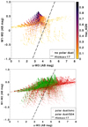 |
Fig. 2. Distribution of composite models in the u-W3, W1-W2 color plot. The models are created with X-CIGALE for an AGN type 1 and a host galaxy from z = 0 to z = 2.5. Top panel: no obscuration by polar dust is considered. The relative contribution of both components defined by the fraction of the dust luminosity coming from the AGN is color coded. Bottom panel: polar dust obscuration is added. Models generated with the SMC (resp., G04) extinction curve are plotted as red (resp., green). The SMC extinction curve leads to a larger reddening of the u-W3 color. All magnitudes are in AB units and the line boundary defined by Hickox et al. (2017) to identify obscured quasars is modified accordingly (u − W3 = 1.4 × (W1 − W2) + 4.1). The number of G04 models is reduced by a factor of 2 on the figure for a better visibility for both distributions. |
3. Analysis of BLAGN from the XMM-XXL survey
3.1. Sample
The X-ray AGN sample used in this work comes from the XMM-XXL survey (Pierre et al. 2016). This survey has a medium depth of ∼6 × 10⁻¹⁵ erg cm−2 s−1 and an exposure time of ∼10 ks per XMM pointing. The field covers a total area of 50 deg2 split into two nearly equal extragalactic sub-regions. In this study, we use the XXL North sample that consists of 8445 X-ray sources (Liu et al. 2016). Spectroscopic redshifts and spectral classification are given by Menzel et al. (2016) for 2512 of these sources. In our analysis, we start with the 1637 BLAGN of the Menzel et al. catalog, with a spectroscopic redshift lower than 2.5. Intrinsic X-ray fluxes are taken from Mountrichas et al. (2021b).
The available photometry is described in Sect. 2 of Mountrichas et al. (2021b). In summary, all our sources have u,g,r,i,z photometry from the Sloan Digital Sky Survey (SDSS). Near-IR photometry (J,H,K) is available for 836 sources from the Visible and Infrared Survey Telescope for Astronomy (VISTA; Emerson et al. (2006). Mid-IR photometry comes from Spitzer (IRAC and MIPS) and allWISE (Wright et al. 2010) datasets. Spitzer data are provided by the HELP collaboration (Shirley et al. 2021). The wavelength coverage of WISE and IRAC is crucial to identify AGN and we reduce the sample to the 1523 sources detected with either IRAC1 or W1, and IRAC2 or W2, by order of priority. We ensure a mid-IR coverage by selecting sources with at least one measured flux in either W3, W4, or MIPS13. We are left with 1275 sources. Herschel/SPIRE fluxes for 824 of these sources come from the HELP project4. Only SPIRE fluxes were included in the analysis because of the much lower sensitivity of the PACS observation in the XMM-XXL field (Oliver et al. 2012).
3.2. SED fitting and SFR and Mstar estimations
In Fig. 3, we compare the color distributions of models and data in the same color plot as was previously used to show the models in Fig. 2. To plot the W1-W2 color, we use either IRAC or WISE data without applying any correction which are less than 0.2 mag (e.g., Richards et al. 2015). The set of models is found to cover the observed colors. The need to introduce a reddening of the AGN emission for at least a fraction of the sources is clearly set out when Fig. 3 is compared to the distributions of models in Fig. 2.
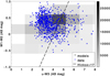 |
Fig. 3. Models compared to data in the u − W3, W1 − W2 color diagram. The density of models created with X-CIGALE is plotted with a gray scale and the observed colors in blue. W1−W2 is calculated with IRAC or WISE fluxes, by order of preference. |
Three different fits are performed with the models described in Sect. 2: without polar dust and with a polar dust component described by an SMC extinction curve and then a G04. The global quality of the fit is assessed by the χ2 value of the best fit and by a reduced  , defined as the χ2/(N − 1) with N being the number of data points5. The values of input and output parameters and their corresponding uncertainties are estimated as the likelihood weighted means and standard deviations. To exclude badly fitted SEDs, we only consider sources for which at least one of the three fits correspond to
  < 5; thus, 1212 (95%) sources fulfill this condition. Our conclusions are unchanged, with a limit set at
  < 3 (1030 sources).
In the next sub-section, we compare the three fits using the Bayesian information criterium (BIC), defined as BIC = χ2 + k × ln(N), where k is the number of free parameters (Ciesla et al. 2018; Buat et al. 2019). BIC scores a model on its likelihood and complexity: a penalty is put on the model with the highest number of free parameters and the model with the lowest BIC is prefered. When polar dust obscuration is considered with a fixed extinction curve, two free parameters are added (dust temperature and color excess), as compared to the fit without polar dust.
Our sample spans a large range of redshifts, and performing a single modeling of the SFH (cf. Table 1) would not correctly describe the bulk of the stellar content. In order to test the validity of our single fit, we tested another set of parameters for the SFH. We defined five redshift bins from z = 0 to 2.5 and in each bin we defined an age for the main stellar population in each bin close to the age of the Universe. A recent burst was added in a similar way as for the first fit. The results of our study were found unchanged with regard to the need to account for polar dust and for the best extinction curve to model it. The SFR and stellar mass (Mstar) estimates were also found to be similar. For the sake of simplicity, we kept our single model of SFH with a large set of input parameters.
Using mock data generated with X-CIGALE, Mountrichas et al. (2021b) checked the robustness of measurements of SFR and Mstar measurements for samples of AGN galaxies with similar redshift range and wavelength coverage. These authors also tested the effect of considering or not SPIRE data on SFR measurements. We performed all these checks for our sub-sample of BLAGN and reached similar conclusions, attesting the robustness of SFR and Mstar determinations.
To further exclude unreliable estimations of SFR and Mstar, we applied the same method as Mountrichas et al. (2021b) and compared the value of the best model with the likelihood weighted mean value calculated by X-CIGALE. A large difference between them means that the probability density function is either ill-defined or very asymmetric, in both cases the estimation of the corresponding parameter is not satisfying. Therefore, in the following, we consider only measurements corresponding to |log(SFRbest/SFRbayes)| < 0.5 dex and  dex.
dex.
3.3. Polar dust component
We focus now on the study of polar dust, by first defining sources for which this component is needed (or not) to substantially improve the fit and, in a second step, determining which extinction curve is preferred.
3.3.1. Selection of sources according to the polar dust component
To compare our fits and select a model, we calculate the difference of BIC between pairs of models (SMC and no polar dust; G04 and no polar dust; SMC and G04) for our 1212 sources. We adopt the criterium of positive evidence against the model with the highest BIC when Δ(BIC) > 2 (positive evidence) (Kass & Raftery 1995). We find a positive evidence against no polar dust for 347 objects (29%). We also select sources for which no polar dust is needed to fit their SED. The models we are comparing are nested: models with polar dust and E(B − V)pd = 0 correspond to models without polar dust. Thus, we consider that no polar dust is needed when both best values of E(B − V)pd with either SMC or G04 are found equal to 0 [e.g.,][]Aufort2020, it is the case for 332 sources (27%). Nothing can be concluded for 44% of the sample.
Among the 347 sources that are better described with polar dust, an SMC extinction curve is preferred (as a positive evidence against G04) for 50% of them (173 sources). Only 21% (72 sources) correspond to a G04 curve and there is no significant difference between the two extinction curves for the remaining 29%.
We compare these numbers to those found when only sources with SPIRE data are considered. With this restricted sample of 790 sources, no polar dust is needed for 22% of the sources, while 31% show positive evidence against no polar dust with a repartition between either SMC (44%) and G04 (26%) extinction curves. These percentages are close the ones we find with the full sample.
In the following, for the sake of clarity, we define a BLAGN with polar dust as one of the 347 sources with a positive evidence against no polar dust; 173 will be considered as described with an SMC law and 72 with a G04 law (i.e., only 71% of BLAGN with polar dust will have an assigned extinction law). The subsample defined as BLAGN without polar dust will consist of the 332 sources best fitted with E(B − V)pd = 0 for each polar dust model. In Fig. 4, these different subsamples are plotted in the u-W3, W1-W2 plane. It can be seen that most of the BLAGN sources populating the upper right region are found with a polar dust and an SMC extinction curve: a strong reddening is needed to shift the u-W3 color of these sources from the locus without polar dust to the observed values. Sources that are better characterized by the presence of polar dust and the much flatter G04 extinction curve are predominantly found in the left region of Fig. 4, where models without polar dust also lie: the color reddening is strongly reduced with the G04 law as shown in Fig. 2. The status of the polar dust component for each of the 1212 sources is listed in Table A.1, the full version of the table is available at the CDS.
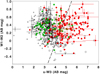 |
Fig. 4. Distribution of our BLAGN sample in the same color plot as in Fig. 2. Sources for which a polar dust component is not needed are represented with crosses, sources better fitted with a polar dust component are plotted with circles. Green circles are for sources better fitted with a G04 extinction curve, red circles for sources better fitted with an SMC extinction curve, open circles sources for which the extinction curve cannot be determined. Sources populating the upper right side of the plot are predominantly found with a polar dust characterized by the SMC extinction curve, the reddening of the u − W3 color is strongly reduced with the G04 extinction curve. Magnitudes are in AB units and the dotted line represents the boundary defined by Hickox et al. (2017) and modified accordingly (u − W3 = 1.4(W1 − W2) + 4.1). Uncertainties in the measured colors are over-plotted for one source randomly selected over five to avoid crowding. |
3.3.2. Statistical corrections from a mock analysis
In order to further check the validity of our results on the introduction of the polar dust component, we performed a specific mock analysis with the full dataset. We used the X-CIGALE option to create a mock dataset from the best SED of each fit for the three subsamples of sources without polar dust, with polar dust modeled with the SMC law, and with polar dust modeled with the G04 law. The code uses the best flux of each source and adds a random noise extracted from a Gaussian distribution with the same standard deviation as for the observed flux. We merged the three datasets in a single mock catalog. This simulated catalog is fitted with the same strategy as for the observed sample (cf. Sect. 3.2). We performed the selection of sources as described in Sect. 3.3.1: we chose the mock sources with positive evidence against no polar dust and described either by SMC or G04 extinction law, as well as the sources whose best fit of their SED corresponds to no polar dust.
52% of the input catalog created without polar dust is confirmed with no polar dust. The percentage of successful identifications of input sources with polar dust is 60%. Nothing can be concluded for 48% (resp. 40%) of sources built without polar dust (resp. with polar dust). The number of misidentifications is very low, with less than 2% of mock sources with polar dust classified without polar dust and no mock source without polar dust classified with polar dust. From this mock analysis, we conclude that the fraction of observed BLAGN classified with and without polar dust are likely to be similar since the fractions measured are similar (29% and 27%, respectively) and the corrections to apply to both populations close to each other (respectively 60% and 52% of sources recovered). Applying these corrections to the observed fractions leads to ≃50% of sources either with or without polar dust.
The distinction between SMC and G04 extinction curves is also investigated with our simulated sample. The percentage of mock sources created with the G04 law and identified successfully is 44%, the percentage reaches 67% for the SMC law. If we account for the full process of selection (evidence for or against polar dust and then distinction between G04 and SMC laws), the identification of the true extinction law is successful for 49% of the input sources with the SMC curve against 31% for the G04 curve. This analysis confirms the difficulty in identifying polar dust characterized by a gray extinction curve. If we apply the corrections drawn from our mock analysis to correct the numbers of sources observed with SMC o G04 law (173 and 72, respectively), we find that 60% of the sources with polar dust should be characterized by a steep (SMC) law and 40% with a flat (G04) law.
3.3.3. Impact of the extinction curve
The G04 law can be considered as an extreme, it was derived for radio-loud AGN and is flatter than other curves derived on different AGN and quasar populations (e.g., Czerny et al. 2004). In this section, we investigate the impact of the adopted extinction curves by adopting the average extinction curve proposed by Gaskell & Benker (2007) to supersede the G04 law (hereafter, the GB07 law).
We performed the same analysis as in Sect. 3.3.1, this time with the SMC and GB07 laws. The percentage of sources whose SED is better described with or without polar dust are only slightly modified: it increases from 27% to 33% for sources without polar dust and is found nearly unchanged for sources with polar dust (28% to 27%). The slight increase of sources for which no polar dust is needed comes from the way we select these sources, when the best values E(B − V)pd of both fits with polar dust is equal to 0 (cf. Sect. 3.3.1). Adopting the GB07 law leads to more reddening than with the G04 law for a given E(B − V)pd: some sources for which only a very small reddening is acceptable can be best fitted with G04 and a low value E(B − V)pd; but not with GB07, for which the best fit corresponds to E(B − V)pd = 0.
As expected, the assignment of a dust extinction curve, either steep (SMC) or flat (G04 and GB07), is found to depend on the curves considered for the fits. When we use the SMC and GB07 laws, 43% (134 sources) of sources with polar dust are described as SMC against 50% (173 sources) with the SMC and G04 laws. No extinction curve can be assigned to the 39 sources described with SMC polar dust in the SMC/G04 fits and not in the SMC/GB07 fit. This result is explained by the smaller difference between the shape of the SMC and GB07 curves than between SMC and G04. For these 39 sources, the best χ2 obtained with GB07 are found lower than with G04. Their polar dust component may be characterized by an extinction curve that is intermediate between SMC and GB07.
The major change we find is for the assignment of the flat law: this is the case for 21% (72 sources) with G04 but for only 7% (24 sources) with GB07. To understand this difference, we analyzed the 72 sources previously described with G04. We could confirm only 47 of them as having polar dust with the SMC/GB07 fit, nothing can be concluded with regard to the presence of polar dust for the remaining 25. Among the 47 sources with polar dust, 20 are found better described with GB07 polar dust, however, no conclusion can be reached for the remaining 27. We conclude that the strong decrease in the number of sources with polar dust described with GB07 is explained by the larger fraction of fits for which no significant difference is found between models with no polar dust and with polar dust, either SMC or GB07. The best χ2 found for the fits of the 72 SEDs with GB07 are systematically higher than with G04. The sources identified with G04 polar dust do not exhibit any substantial reddening, as shown in Fig. 4, and their UV-to-far IR SED is better fitted with a very flat extinction curve.
Obviously, our very simplified comparison of only two laws cannot reflect the large diversity of AGN dust extinction laws reported both at low and high redshift (Crenshaw & Kraemer 2001; Maiolino et al. 2001a; Gaskell & Benker 2007; Gallerani et al. 2010; Gaskell et al. 2016). It is worth noting that such a diversity is also found for the effective attenuation curves for normal galaxies (Salim & Narayanan 2020, and references therein). In our analysis, we cannot separate the effect of polar dust close to the AGN or polar dust that is distributed on larger scales in the host galaxy. In a future work, we plan to implement flexible extinction recipes to study the diversity of polar dust extinction curves and investigate correlations with other characteristics of AGN and host galaxies.
3.3.4. Properties of polar dust
In this part of the study, we go back to our initial fits and results with the SMC and G04 laws and discuss the impact of using the GB07 law. Prior to the analysis of some polar dust properties inferred from our analysis, we recall that we are modeling the component that we call “polar dust,” with a dust screen along the direction perpendicular to the plane of the dusty torus and an extinction calculated with a single extinction curve. This very simple model does not allow us to get any direct information on the local and large-scale distribution of this dusty component distributed in the polar direction.
Here, we discuss two output quantities of our analysis: the amount of extinction in the V-band due to polar dust and the temperature of the polar dust. The estimated values of these two parameters are given in Table A.1 for sources for which an extinction curve is assigned. Parameter estimation with CIGALE is based on Bayesian Inference, assuming Gaussian uncertainties (Walcher et al. 2011, and references therein). The probability distributions of the prior parameters of the models are assumed to be flat and the probability of all models are computed and integrated over all model parameters (except the one to be derived) to build the probability distribution function (PDF) of the posterior. The mean and standard deviation of the PDF yield the parameter estimate and its associated uncertainty. The validity of the measure is also checked by using our mock analysis (cf. Sect. 3.3.2). In Fig. 5, the exact values of these parameters are compared to their estimations obtained by fitting the simulated samples built with each extinction curve. Both parameters are reasonably well retrieved. Large AV values of low statistical significance6 are underestimated. The dispersion of the estimated temperature corresponding to a true value of 100 K is large and its statistical significance is low, but similar for both extinction curves. So we expect that the difference found below between both distributions is real.
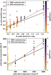 |
Fig. 5. Results of the mock analysis performed for polar dust extinction in the V-band, AV (top panel) and polar dust temperature (bottom panel). The exact values (x-axis) are plotted against the values measured by fitting the simulated datasets (y-axis). The open circles refer to the SMC extinction curve, the filled circles to the G04 extinction curve. The linear fits are shown as solid (G04) and dotted (SMC) lines. The statistical significance of the measure is color-coded. |
3.3.4.1. Dust attenuation and X-ray absorbing column density
In Fig. 6, the obscuration in the V-band due to polar dust, AV, is compared to the X-ray absorbing column density NH measured by Liu et al. (2016)7 for sources described with either an SMC or a G04 law. The AV values are calculated with the color excess E(B − V)pd and RV corresponding to either the SMC or the G04 curve (cf. Sect. 2.1). AV are found lower in average for the SMC curve with all values lower than 1 mag, than for the G04 curve for which values extend up to 1.6 mag. This difference is explained by the shapes of the extinction curves: with an SMC curve the extinction in UV (∼150 nm) is four times higher than in the V-band when both extinctions are similar with the G04 curve. Therefore, the total amount of energy absorbed by dust is more efficient with a steep extinction curve than with a flat curve for a given AV. Here, we also plot the AV values corresponding to the 24 sources better fitted with the GB07 law (Sect. ), with their distribution overlapping the one found with SMC, which is as expected since this law corresponds to a lower RV value.
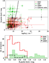 |
Fig. 6. V-band attenuation AV due to the AGN polar dust component. Top panel: AV is plotted against the X-ray absorbing column density NH for sources with polar dust described either with the SMC law (red circles) or the G04 law (green points). AV is also plotted for the 24 sources that are found to be consistent with the GB07 law (black triangles). Uncertainties on AV measurements (1σ dispersion estimated by X-CIGALE) and NH (16th and 84th percentiles of the distribution) are over-plotted (for only one source with SMC law randomly selected over 3). The Galactic value of AV/NH is indicated as a black line. Bottom panel: AV distribution for sources described with each law. |
We do not find any correlation between AV and NH, but our sample is restricted to BLAGN with a narrow range of column densities (NH < 1021.5 cm−2 for most of the sources). The AV/NH ratios are distributed above and below the standard Galactic value (AV/NH = 5.3210−22 mag cm−2 from Bohlin et al. (1978) with a standard Galactic RV = 3.1). All our sources with an X-ray column density larger than 1021.5 cm−2 have AV/NH ratios lower than Galactic. 34% of the sources with an SMC curve have higher AV/NH than Galactic and the percentage reaches 80% with a G04 extinction law but, as mentioned above, the comparison between the G04 and Galactic laws is difficult because of RV difference. We note that the uncertainty in NH is also large, even without accounting for X-ray variability. Using the value corresponding to the 84th percentile of the distribution reduces the fraction of sources above Galactic to 7% (resp. 30%) for the SMC (resp. G04) law.
The correlation between optical extinction and X-ray absorption is well established from unabsorbed type 1 AGN to optically obscured type 2 AGN although with a large dispersion (e.g., Goodrich et al. 1994; Burtscher et al. 2016). Jaffarian & Gaskell (2020) found that the large scatter in the relation they found between the color excess E(B − V) and NH for BLAGN could be explained by the variability of the X-ray column densities (see also Burtscher et al. 2016).
Maiolino et al. (2001a) reported AV/NH values in average lower than Galactic in various classes of AGN with broad emission lines and NH > 1021.5 cm−2. The only three sources in their sample with NH < 1021.5 cm−2 have an AV/NH ratio that is about four times higher than Galactic, but with low X-ray luminosity. Burtscher et al. (2016) measured AV/NH for 25 local X-ray detected source and found values close to or lower than Galactic. The ratios for their sources with NH ≤ ∼ 1021 cm−2 (and corresponding to Seyfert type 1 to 1.5) are found consistent with the Galactic value, although they show that variability of NH makes the results uncertain.
The physical context to interpret these observations is also extremely complex. Several processes are rivaling to modify the size distributions of dust grains: grain-grain collisions, with shattering and coagulation, and grain growth (accretion) on gas phase metals (e.g., Asano et al. 2013). All of them have an impact on both the shape of the extinction curve and the dust to gas ratio for a similar initial dust composition and size distribution. Hirashita (2012) showed that coagulation flattens the extinction curve and grain growth increases the steepness of the extinction curve in the UV and the amplitude of the bump at 2175 nm for an initial Galactic dust composition. Accretion and coagulation have different effects on the extinction cross section per H atom and consequently on the AV/NH ratio, which also depends on the initial and final distributions of grains sizes (e.g., Cardelli et al. 1989; Maiolino et al. 2001a). The depletion of small grains can occur in the vicinity of the AGN, small grains being expelled by strong winds (Gaskell et al. 2004). Last but not least, radiation transfer can make the situation even more complex. Scicluna & Siebenmorgen (2015) showed that radiation transfer effects inside an observing beam that encompasses a dusty medium may also alter the effective extinction curve without any change in dust grain composition and are able to reproduce any RV values.
3.3.4.2. Polar dust temperature
The temperature of the modified black body describing the emission of polar dust is a free parameter of our fitting process. The distributions of values found for the two sub-samples described with either an SMC or a G04 extinction curve are shown in Fig. 7. Lower temperatures are found for polar dust better described with the SMC law than with the G04 law. The temperatures found with the G04 law extend over the full range of initial values (from 100 to 2000 K) when 78% of the temperatures for the SMC law are found lower than 500 K. Very similar distributions are found when the sample is reduced to sources detected with Herschel as well as using the GB07 extinction curve instead of G04 (cf. Sect. 3.3.4). The higher temperatures found with the G04 curve are likely to be more easily found close to the AGN, but they are not high enough for a destruction of small grains by sublimation.
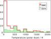 |
Fig. 7. Distribution of polar dust temperatures of sources with polar dust described either with the SMC law (red line) or the G04 law (green filled histogram). |
A steep extinction curve, modeled with the SMC law in this work, could be explained by the presence of a foreground, optical thin shell (Witt & Gordon 2000; Scicluna & Siebenmorgen 2015) located at larger distance of the AGN in consistency with the lower temperatures found for the SMC polar dust component.
4. Properties of BLAGN with and without polar dust
In this section, we compare the distributions of redshift, X-ray luminosity, SFR, Mstar, and specific SFR (defined as sSFR = SFR/Mstar) of sources described with polar dust or without polar dust, as defined at the end of Sect. 3.3.1. We restrict the analysis to sources with secure measurements of SFR and Mstar as defined in Sect. 3.2. We are left with 301 sources with no polar dust and 289 sources with polar dust. For sources with polar dust but no clear assignment of an SMC or G04 extinction curve, we adopted the extinction curve giving the lowest χ2. The estimated values of SFR and Mstar are given in Table A.1.
The redshift distribution of sources with and without polar dust is shown in Fig. 8. There is a small excess of sources with polar dust at redshift lower than 1. We performed a two-sample Kolmogorov-Smirnov test and found a p-value equal to 0.03. We account for this difference before comparing other parameters which may evolve with redshift (e.g., Masoura et al. 2018). In each redshift bin, we randomly draw an equal number of sources with and without polar dust, the number of sources from each sub-sample being the lowest observed number in the bin. At the end of the process, we are left with 494 sources instead of the 590 initial ones. The distribution of the X-ray luminosity in the 2–10 keV band8 for the 494 sources, is also shown in Fig. 8. A two-sample Kolmogorov-Smirnov test returns a p-value equal to 0.18 for the LX distributions meaning that they cannot be distinguished.
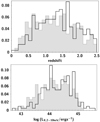 |
Fig. 8. Distributions of redshift and X-ray luminosities for galaxies whose SED is better described with polar dust (filled histogram) and without polar dust (empty histogram). |
We compare SFR, Mstar and sSFR for both sub-samples. These quantities are estimated with X-CIGALE with an uncertainty which depends on the SED of the source. We account for these uncertainties by weighting each measure with its statistical significance. The resulting distributions are shown in Fig. 9. For each considered quantity, the distributions for sources with and without polar dust are found significantly different from a two sample Kolmogorov-Smirnov test, the difference being more pronounced for Mstar (p-value = 0.0002 compared to 0.03 for SFR and sSFR). SFR and Mstar are found shifted toward higher values for sources with polar dust, but mean values of the SFR (resp. Mstar) distributions differ by only 0.08 dex (resp. 0.12 dex). The sSFR distribution of sources without polar dust shows a tail toward low values that is not found for the sources with polar dust, median values of the distributions differ by only 0.05 dex (average values are not considered because the sSFR distributions are obviously not symmetrical). These differences in SFR and Mstar distributions (see also Zou et al. 2019; Mountrichas et al. 2021b) could be interpreted as an increase of dust mass in the sources with polar dust according to well known scaling relations between dust masses, Mstar, and SFR (e.g., Cortese et al. 2012; Santini et al. 2014; da Cunha et al. 2010). This could also serve as an argument in favor of a polar dust distributed over large scales and connected to the interstellar medium of the galaxy. In any case, these results have to be considered tentative and the small difference found between median or mean values of the distributions (∼0.1 dex) is lower than the global expected uncertainty in Mstar and SFR measurements (Mountrichas et al. 2021a,b).
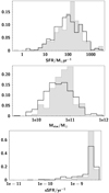 |
Fig. 9. Distributions of SFR, Mstar and sSFR for galaxies with polar dust (filled histogram) and without polar dust (empty histogram). |
5. Impact of the polar dust component on the measurements of physical parameters
Adding a dust absorption to the emission of the active nucleus is expected to have an impact on the contribution of the observed AGN emission to the composite SED and, consequently, to the characteristics of the stellar component. In Fig. 10, we compare the estimated values of Mstar and SFR for the sources with polar dust, when the fit is performed with or without polar dust. When polar dust is not considered, both quantities are systematically overestimated for sources best described with the SMC law. We have seen that the UV to near-IR spectra of the AGN component is substantially reddened with SMC polar dust (Sect. 2, Figs. 2 and 4). When the composite SEDs are fitted without polar dust, the reddening is only possible through the obscuration of the stellar component: its contribution to the SED increases, leading to higher Mstar and SFR. When the polar dust is described with the G04 law, no systematic shift is found since this extinction law does not imply any substantial reddening.
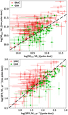 |
Fig. 10. SFR (bottom panel) and Mstar (top panel) estimations and their related uncertainties for sources with polar dust (red dots: SMC law, green dots: G04 law). x-axis: values obtained from the fit with polar dust component, y-axis: values obtained from the fit without polar dust component. |
The SEDs showing evidence against polar dust are selected to have a very low, even null, contribution of polar dust when this component is added (they are selected with best fits having E(B − V)pd = 0, and the likelihood weighted values of E(B − V)pd are all found lower than 0.05 mag). Therefore, performing a fit with a polar dust component includes no polar dust models. Parameter values derived from this fitting process should also be valid for sources without polar dust: by construction, the values corresponding to the best fit will be identical and only slight differences are expected for the likelihood weighted estimations of the parameters.
We now test the reliability of results if only a single fit of the SEDs of all our sources is performed. It is logical to use the SMC curve, since this curve is more often preferred than the G04 curve in our selection process and we showed that its introduction is mandatory to describe highly reddened sources. In Fig. 11, the SFR and Mstar measurements with this single fit are compared to SFR and Mstar values obtained previously for sources with no polar dust or with polar dust described with the G04 polar dust (cf. Sect. 2): the agreement between both measurements is found excellent for sources without polar dust and both parameters are found consistent within 0.3 dex for more than 90% of the sources with a polar dust described with the G04 curve from our initial study. We can conclude that a single fit accounting for a polar dust with the SMC extinction curve gives satisfactory results for measuring the SFR and Mstar of host galaxies with a good accuracy. However such a single fit only allows us to identify a polar dust component characterized by a steep extinction curve. In this work, we show that the identification and the characterization of a polar dust component requires more investigations based on fits performed with different extinction laws.
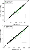 |
Fig. 11. SFR (bottom panel) and Mstar (top panel) estimated from a single fit assuming a polar dust obscuration with an SMC extinction curve, for sources first identified with either polar dust described with a G04 curve (green empty circles) or no polar dust (black dots). x-axis: Parameters estimated from the initial analysis (cf. Sect. 3), y-axis: Parameters estimated with the single fit. The average 1σ uncertainty on the estimated parameters is indicated as a cross. |
6. Summary
In this work, we investigate the presence of dust along the line of sight of BLAGN by using the impact of adding polar dust reddening to their UV to IR continuum. We fit the SEDs of 1275 BLAGN in the XMM-XXL field with X-CIGALE. The code includes a simple model of polar component based on a screen geometry and an extinction curve, which can be chosen either steep (SMC curve of Pei 1992) or almost flat in the UV-optical range (G04 extinction curve of Gaskell et al. 2004). Both curves have a very different impact on the reddening of the AGN continuum, which allows us to compare different configurations.
We found a similar fraction of sources that are better fitted (or not) with the introduction of a polar dust component. A mock analysis conducted to understand the performance of our classification led us to conclude that our sources are probably equally distributed between the two categories. Among the sources identified with a polar dust, 50% are better modeled with an SMC curve against 21% with a G04 law. After corrections from the mock analysis, we concluded that SMC-like curves could represent 60% of sources with polar dust against 40% for flat curves represented by the G04 law. The fraction of sources found with or without polar dust is found nearly unchanged when the GB07 extinction law (Gaskell & Benker 2007) is used instead of G04, but the assignment of an extinction curve either flat or steep depends on the adopted curve. The GB07 extinction curve is not as flat as G04 and makes the differentiation between steep (SMC) and flat (GB07) laws more difficult.
The extinction in the V-band, AV, does not correlate with the X-ray absorbing column density NH. The distribution of AV/NH ratios is broad with values above and below Galactic. The temperatures of the modified black body used for the dust polar re-emission extend over the full range of initial values (from 100 to 2000 K) for the G04 law, but 78% of the temperatures for the SMC law were found to be lower than 500 K. These results could provide some information on the properties of polar dust and its location along the line of sight, although our very simple screen model on the one side and the complex physical processes assumed to be at work on the other side do not allow us to propose a fully consistent picture.
We showed that the fits of the SEDs without including polar dust lead to an overestimation of the stellar component (and, consequently, of SFR and Mstar) of sources with polar dust described by the SMC law. A single fit with X-CIGALE that includes a polar dust component with the SMC extinction curve avoids this issue and returns reliable SFR and Mstar, but this is not sufficient to identify all the sources hosting polar dust.
The Dale et al. (2014) templates are used without AGN contribution which is added with the SKIRTOR module.
To consider only WISE detections we discarded all fluxes with no associated uncertainty.
The Herschel Extragalactic Legacy Project (HELP) is a European funded project to analyze all the cosmological fields observed with the Herschel satellite. The HELP datasets are available on the Herschel database in Marseille (http://hedam.lam.fr/HELP/).
 value is only used as an indication of the global quality of the fit and the best model is not used for the estimation of the parameters.
The statistical significance is defined as the ratio of the estimated value by its 1 σ uncertainty, both given by X-CIGALE.
NH has been calculated by Liu et al. (2016), by applying X-ray spectral modeling and stacking, adopting the Bayesian X-ray Analysis software (BXA, Buchner et al. 2014) to fit the X-ray spectra of individual sources.
Hard X-ray luminosities 2–10 keV from the catalog of Menzel et al. (2016).
Acknowledgments
The project has received funding from Excellence Initiative of Aix-Marseille University – AMIDEX, a French ‘Investissements d’Avenir’ programme. GM acknowledges support by the Agencia Estatal de Investigacíon, Unidad de Excelencia María de Maeztu, ref. MDM-2017-0765. M.S. acknowledges support by the Ministry of Education, Science and Technological Development of the Republic of Serbia through the contract no. 451-03-9/2021-14/200002 and by the Science Fund of the Republic of Serbia, PROMIS 6060916, BOWIE.
References
- Antonucci, R. 1993, ARA&A, 31, 473 [Google Scholar]
- Asano, R. S., Takeuchi, T. T., Hirashita, H., & Nozawa, T. 2013, MNRAS, 432, 637 [NASA ADS] [CrossRef] [Google Scholar]
- Asmus, D. 2019, MNRAS, 489, 2177 [NASA ADS] [CrossRef] [Google Scholar]
- Asmus, D., Hönig, S. F., & Gandhi, P. 2016, ApJ, 822, 109 [NASA ADS] [CrossRef] [Google Scholar]
- Assef, R. J., Kochanek, C. S., Brodwin, M., et al. 2010, ApJ, 713, 970 [NASA ADS] [CrossRef] [Google Scholar]
- Aufort, G., Ciesla, L., Pudlo, P., & Buat, V. 2020, A&A, 635, A136 [NASA ADS] [CrossRef] [EDP Sciences] [Google Scholar]
- Baes, M., & Camps, P. 2015, Astron. Comput., 12, 33 [NASA ADS] [CrossRef] [Google Scholar]
- Bohlin, R. C., Savage, B. D., & Drake, J. F. 1978, ApJ, 224, 132 [NASA ADS] [CrossRef] [Google Scholar]
- Boquien, M., Burgarella, D., Roehlly, Y., et al. 2019, A&A, 622, A103 [NASA ADS] [CrossRef] [EDP Sciences] [Google Scholar]
- Bruzual, G., & Charlot, S. 2003, MNRAS, 344, 1000 [NASA ADS] [CrossRef] [Google Scholar]
- Buat, V., Boquien, M., Małek, K., et al. 2018, A&A, 619, A135 [NASA ADS] [CrossRef] [EDP Sciences] [Google Scholar]
- Buat, V., Ciesla, L., Boquien, M., Małek, K., & Burgarella, D. 2019, A&A, 632, A79 [NASA ADS] [CrossRef] [EDP Sciences] [Google Scholar]
- Buchner, J., Georgakakis, A., Nandra, K., et al. 2014, A&A, 564, A125 [NASA ADS] [CrossRef] [EDP Sciences] [Google Scholar]
- Burtscher, L., Davies, R. I., Graciá-Carpio, J., et al. 2016, A&A, 586, A28 [NASA ADS] [CrossRef] [EDP Sciences] [Google Scholar]
- Calistro Rivera, G., Alexander, D. M., Rosario, D. J., et al. 2021, A&A, 649, A102 [NASA ADS] [CrossRef] [EDP Sciences] [Google Scholar]
- Calzetti, D., Armus, L., Bohlin, R. C., et al. 2000, ApJ, 533, 682 [NASA ADS] [CrossRef] [Google Scholar]
- Cardelli, J. A., Clayton, G. C., & Mathis, J. S. 1989, ApJ, 345, 245 [NASA ADS] [CrossRef] [Google Scholar]
- Carleton, N. P., Elvis, M., Fabbiano, G., et al. 1987, ApJ, 318, 595 [NASA ADS] [CrossRef] [Google Scholar]
- Casey, C. M. 2012, MNRAS, 425, 3094 [Google Scholar]
- Chabrier, G. 2003, PASP, 115, 763 [Google Scholar]
- Chen, C.-C., Smail, I., Swinbank, A. M., et al. 2015, ApJ, 799, 194 [NASA ADS] [CrossRef] [Google Scholar]
- Ciesla, L., Elbaz, D., Schreiber, C., Daddi, E., & Wang, T. 2018, A&A, 615, A61 [NASA ADS] [CrossRef] [EDP Sciences] [Google Scholar]
- Cortese, L., Ciesla, L., Boselli, A., et al. 2012, A&A, 540, A52 [NASA ADS] [CrossRef] [EDP Sciences] [Google Scholar]
- Crenshaw, D. M., & Kraemer, S. B. 2001, ApJ, 562, L29 [NASA ADS] [CrossRef] [Google Scholar]
- Czerny, B., Li, J., Loska, Z., & Szczerba, R. 2004, MNRAS, 348, L54 [NASA ADS] [CrossRef] [Google Scholar]
- da Cunha, E., Eminian, C., Charlot, S., & Blaizot, J. 2010, MNRAS, 403, 1894 [NASA ADS] [CrossRef] [Google Scholar]
- Dale, D. A., Helou, G., Magdis, G. E., et al. 2014, ApJ, 784, 83 [NASA ADS] [CrossRef] [Google Scholar]
- Donley, J. L., Koekemoer, A. M., Brusa, M., et al. 2012, ApJ, 748, 142 [Google Scholar]
- Elvis, M., Hao, H., Civano, F., et al. 2012, ApJ, 759, 6 [NASA ADS] [CrossRef] [Google Scholar]
- Elvis, M., Wilkes, B. J., McDowell, J. C., et al. 1994, ApJS, 95, 1 [Google Scholar]
- Emerson, J., McPherson, A., & Sutherland, W. 2006, The Messenger, 126, 41 [NASA ADS] [Google Scholar]
- Fuller, L., Lopez-Rodriguez, E., Packham, C., et al. 2019, MNRAS, 483, 3404 [NASA ADS] [CrossRef] [Google Scholar]
- Gallerani, S., Maiolino, R., Juarez, Y., et al. 2010, A&A, 523, A85 [NASA ADS] [CrossRef] [EDP Sciences] [Google Scholar]
- Gaskell, C. M., & Benker, A. J. 2007, ArXiv e-prints [arXiv:0711.1013] [Google Scholar]
- Gaskell, C. M., Goosmann, R. W., Antonucci, R. R. J., & Whysong, D. H. 2004, ApJ, 616, 147 [NASA ADS] [CrossRef] [Google Scholar]
- Gaskell, C. M., Gill, J. J. M., & Singh, J. 2016, ArXiv e-prints [arXiv:1611.03733] [Google Scholar]
- Goodrich, R. W., Veilleux, S., & Hill, G. J. 1994, ApJ, 422, 521 [NASA ADS] [CrossRef] [Google Scholar]
- Hao, H., Elvis, M., Bongiorno, A., et al. 2013, MNRAS, 434, 3104 [NASA ADS] [CrossRef] [Google Scholar]
- Hickox, R. C., Myers, A. D., Greene, J. E., et al. 2017, ApJ, 849, 53 [NASA ADS] [CrossRef] [Google Scholar]
- Hirashita, H. 2012, MNRAS, 422, 1263 [NASA ADS] [CrossRef] [Google Scholar]
- Hönig, S. F., & Kishimoto, M. 2017, ApJL, 838, 20 [Google Scholar]
- Hopkins, P. F., Strauss, M. A., Hall, P. B., et al. 2004, AJ, 128, 1112 [NASA ADS] [CrossRef] [Google Scholar]
- Jaffarian, G. W., & Gaskell, C. M. 2020, MNRAS, 493, 930 [NASA ADS] [CrossRef] [Google Scholar]
- Kass, R. E., & Raftery, A. E. 1995, J. Am. Stat. Assoc., 90, 773 [CrossRef] [Google Scholar]
- Komatsu, E., Smith, K. M., Dunkley, J., et al. 2011, ApJS, 192, 18 [NASA ADS] [CrossRef] [Google Scholar]
- Laor, A., & Draine, B. T. 1993, ApJ, 402, 441 [NASA ADS] [CrossRef] [Google Scholar]
- Liu, Z., Merloni, A., Georgakakis, A., et al. 2016, MNRAS, 459, 1602 [NASA ADS] [CrossRef] [Google Scholar]
- López-Gonzaga, N., Burtscher, L., Tristram, K. R. W., Meisenheimer, K., & Schartmann, M. 2016, A&A, 591, A47 [NASA ADS] [CrossRef] [EDP Sciences] [Google Scholar]
- Lyu, J., & Rieke, G. H. 2018, ApJ, 866, 92 [NASA ADS] [CrossRef] [Google Scholar]
- Lyu, J., Hao, L., & Li, A. 2014, ApJL, 792, 9 [Google Scholar]
- Maiolino, R., Marconi, A., & Oliva, E. 2001a, A&A, 365, 37 [NASA ADS] [CrossRef] [EDP Sciences] [Google Scholar]
- Maiolino, R., Marconi, A., Salvati, M., et al. 2001b, A&A, 365, 28 [NASA ADS] [CrossRef] [EDP Sciences] [Google Scholar]
- Masoura, V. A., Mountrichas, G., Georgantopoulos, I., et al. 2018, A&A, 618, A31 [NASA ADS] [CrossRef] [EDP Sciences] [Google Scholar]
- Menzel, M. L., Merloni, A., Georgakakis, A., et al. 2016, MNRAS, 457, 110 [NASA ADS] [CrossRef] [Google Scholar]
- Mountrichas, G., Georgakakis, A., Menzel, M. L., et al. 2016, MNRAS, 457, 4195 [NASA ADS] [CrossRef] [Google Scholar]
- Mountrichas, G., Buat, V., Georgantopoulos, I., et al. 2021a, A&A, 653, A70 [NASA ADS] [CrossRef] [EDP Sciences] [Google Scholar]
- Mountrichas, G., Buat, V., Yang, G., et al. 2021b, A&A, 646, A29 [EDP Sciences] [Google Scholar]
- Netzer, H. 2015, ARA&A, 53, 365 [Google Scholar]
- Noll, S., Burgarella, D., Giovannoli, E., et al. 2009, A&A, 507, 1793 [NASA ADS] [CrossRef] [EDP Sciences] [Google Scholar]
- Oliver, S. J., Bock, J., Altieri, B., et al. 2012, MNRAS, 424, 1614 [NASA ADS] [CrossRef] [Google Scholar]
- Pei, Y. C. 1992, ApJ, 395, 130 [Google Scholar]
- Pierre, M., Pacaud, F., Adami, C., et al. 2016, A&A, 592, A1 [NASA ADS] [CrossRef] [EDP Sciences] [Google Scholar]
- Prieto, M. A., Reunanen, J., Tristram, K. R. W., et al. 2010, MNRAS, 402, 724 [NASA ADS] [CrossRef] [Google Scholar]
- Richards, G. T., Hall, P. B., Vanden Berk, D. E., et al. 2003, AJ, 126, 1131 [NASA ADS] [CrossRef] [Google Scholar]
- Richards, G. T., Strauss, M. A., Fan, X., et al. 2006, AJ, 131, 2766 [Google Scholar]
- Richards, G. T., Myers, A. D., Peters, C. M., et al. 2015, ApJS, 219, 39 [NASA ADS] [CrossRef] [Google Scholar]
- Salim, S., & Narayanan, D. 2020, ARA&A, 58, 529 [NASA ADS] [CrossRef] [Google Scholar]
- Santini, P., Maiolino, R., Magnelli, B., et al. 2014, A&A, 562, A30 [NASA ADS] [CrossRef] [EDP Sciences] [Google Scholar]
- Scicluna, P., & Siebenmorgen, R. 2015, A&A, 584, A108 [NASA ADS] [CrossRef] [EDP Sciences] [Google Scholar]
- Shirley, R., Duncan, K., Campos Varillas, M. C., et al. 2021, MNRAS, in press [Google Scholar]
- Stalevski, M., Fritz, J., Baes, M., Nakos, T., & Popović, L. Č. 2012, MNRAS, 420, 2756 [NASA ADS] [CrossRef] [Google Scholar]
- Stalevski, M., Ricci, C., Ueda, Y., et al. 2016, MNRAS, 458, 2288 [NASA ADS] [CrossRef] [Google Scholar]
- Stalevski, M., Asmus, D., & Tristram, K. R. W. 2017, MNRAS, 472, 3854 [NASA ADS] [CrossRef] [Google Scholar]
- Stalevski, M., Tristram, K. R. W., & Asmus, D. 2019, MNRAS, 484, 3334 [NASA ADS] [CrossRef] [Google Scholar]
- Stern, D., Eisenhardt, P., Gorjian, V., et al. 2005, ApJ, 631, 163 [NASA ADS] [CrossRef] [Google Scholar]
- Toba, Y., Ueda, Y., Gandhi, P., et al. 2021, ApJ, 912, 91 [NASA ADS] [CrossRef] [Google Scholar]
- Urry, C. M., & Padovani, P. 1995, PASP, 107, 803 [NASA ADS] [CrossRef] [Google Scholar]
- Walcher, J., Groves, B., Budavári, T., & Dale, D. 2011, Ap&SS, 331, 1 [NASA ADS] [CrossRef] [Google Scholar]
- Witt, A. N., & Gordon, K. D. 2000, ApJ, 528, 799 [Google Scholar]
- Wright, E. L., Eisenhardt, P. R. M., Mainzer, A. K., et al. 2010, AJ, 140, 1868 [Google Scholar]
- Yang, G., Boquien, M., Buat, V., et al. 2020, MNRAS, 491, 740 [NASA ADS] [CrossRef] [Google Scholar]
- Zou, F., Yang, G., Brandt, W. N., & Xue, Y. 2019, ApJ, 878, 11 [Google Scholar]
Appendix A: XCIGALE results for individual sources
Properties derived for each of the 1212 sources with good XCIGALE fits.
All Tables
X-CIGALE modules and input variable parameters used to create the stellar and AGN components of the composite models.
All Figures
|
Fig. 1. SED of the AGN component modeled as described in Sect. 2.2. The scale of the fluxes is arbitrary. The red lines correspond to a polar dust obscuration of the accretion disk emission with an SMC extinction curve, the dust emission is the sum of torus and polar dust emission at 500 K (red solid line) and 100 K (dashed line). The green line corresponds to a polar dust obscuration with a G04 extinction curve. All models are normalized to the same energy emitted by dust. The SED of the model without polar dust is shown as a blue short-dashed line, in this case the dust emission comes only from the dusty torus and the emission of accretion disk is unabsorbed along the line of sight. |
| In the text | |
|
Fig. 2. Distribution of composite models in the u-W3, W1-W2 color plot. The models are created with X-CIGALE for an AGN type 1 and a host galaxy from z = 0 to z = 2.5. Top panel: no obscuration by polar dust is considered. The relative contribution of both components defined by the fraction of the dust luminosity coming from the AGN is color coded. Bottom panel: polar dust obscuration is added. Models generated with the SMC (resp., G04) extinction curve are plotted as red (resp., green). The SMC extinction curve leads to a larger reddening of the u-W3 color. All magnitudes are in AB units and the line boundary defined by Hickox et al. (2017) to identify obscured quasars is modified accordingly (u − W3 = 1.4 × (W1 − W2) + 4.1). The number of G04 models is reduced by a factor of 2 on the figure for a better visibility for both distributions. |
| In the text | |
|
Fig. 3. Models compared to data in the u − W3, W1 − W2 color diagram. The density of models created with X-CIGALE is plotted with a gray scale and the observed colors in blue. W1−W2 is calculated with IRAC or WISE fluxes, by order of preference. |
| In the text | |
|
Fig. 4. Distribution of our BLAGN sample in the same color plot as in Fig. 2. Sources for which a polar dust component is not needed are represented with crosses, sources better fitted with a polar dust component are plotted with circles. Green circles are for sources better fitted with a G04 extinction curve, red circles for sources better fitted with an SMC extinction curve, open circles sources for which the extinction curve cannot be determined. Sources populating the upper right side of the plot are predominantly found with a polar dust characterized by the SMC extinction curve, the reddening of the u − W3 color is strongly reduced with the G04 extinction curve. Magnitudes are in AB units and the dotted line represents the boundary defined by Hickox et al. (2017) and modified accordingly (u − W3 = 1.4(W1 − W2) + 4.1). Uncertainties in the measured colors are over-plotted for one source randomly selected over five to avoid crowding. |
| In the text | |
|
Fig. 5. Results of the mock analysis performed for polar dust extinction in the V-band, AV (top panel) and polar dust temperature (bottom panel). The exact values (x-axis) are plotted against the values measured by fitting the simulated datasets (y-axis). The open circles refer to the SMC extinction curve, the filled circles to the G04 extinction curve. The linear fits are shown as solid (G04) and dotted (SMC) lines. The statistical significance of the measure is color-coded. |
| In the text | |
|
Fig. 6. V-band attenuation AV due to the AGN polar dust component. Top panel: AV is plotted against the X-ray absorbing column density NH for sources with polar dust described either with the SMC law (red circles) or the G04 law (green points). AV is also plotted for the 24 sources that are found to be consistent with the GB07 law (black triangles). Uncertainties on AV measurements (1σ dispersion estimated by X-CIGALE) and NH (16th and 84th percentiles of the distribution) are over-plotted (for only one source with SMC law randomly selected over 3). The Galactic value of AV/NH is indicated as a black line. Bottom panel: AV distribution for sources described with each law. |
| In the text | |
|
Fig. 7. Distribution of polar dust temperatures of sources with polar dust described either with the SMC law (red line) or the G04 law (green filled histogram). |
| In the text | |
|
Fig. 8. Distributions of redshift and X-ray luminosities for galaxies whose SED is better described with polar dust (filled histogram) and without polar dust (empty histogram). |
| In the text | |
|
Fig. 9. Distributions of SFR, Mstar and sSFR for galaxies with polar dust (filled histogram) and without polar dust (empty histogram). |
| In the text | |
|
Fig. 10. SFR (bottom panel) and Mstar (top panel) estimations and their related uncertainties for sources with polar dust (red dots: SMC law, green dots: G04 law). x-axis: values obtained from the fit with polar dust component, y-axis: values obtained from the fit without polar dust component. |
| In the text | |
|
Fig. 11. SFR (bottom panel) and Mstar (top panel) estimated from a single fit assuming a polar dust obscuration with an SMC extinction curve, for sources first identified with either polar dust described with a G04 curve (green empty circles) or no polar dust (black dots). x-axis: Parameters estimated from the initial analysis (cf. Sect. 3), y-axis: Parameters estimated with the single fit. The average 1σ uncertainty on the estimated parameters is indicated as a cross. |
| In the text | |
Current usage metrics show cumulative count of Article Views (full-text article views including HTML views, PDF and ePub downloads, according to the available data) and Abstracts Views on Vision4Press platform.
Data correspond to usage on the plateform after 2015. The current usage metrics is available 48-96 hours after online publication and is updated daily on week days.
Initial download of the metrics may take a while.