| Issue |
A&A
Volume 654, October 2021
|
|
|---|---|---|
| Article Number | L8 | |
| Number of page(s) | 9 | |
| Section | Letters to the Editor | |
| DOI | https://doi.org/10.1051/0004-6361/202141611 | |
| Published online | 18 October 2021 | |
Letter to the Editor
SUPER
VI. A giant molecular halo around a z∼2 quasar
1
Institute of Theoretical Astrophysics, University of Oslo, PO Box 1029, Blindern 0315 Oslo, Norway
e-mail: This email address is being protected from spambots. You need JavaScript enabled to view it.
2
European Southern Observatory, Karl-Schwarzschild-Str. 2, 85748 Garching bei München, Germany
3
Department of Physics and Astronomy, University College London, London WC1E 6BT, UK
4
European Southern Observatory, Alonso de Cordova 3107, Casilla 19, 19001 Santiago, Chile
5
Centro de Astrobiología (CSIC-INTA), Ctra. de Ajalvir, Km 4, 28850 Torrejón de Ardoz, Madrid, Spain
6
INAF – Osservatorio Astronomico di Trieste, Via G. B. Tiepolo 11, 34143 Trieste, Italy
7
Scuola Normale Superiore, Piazza dei Cavalieri 7, 56126 Pisa, Italy
8
INAF – Osservatorio Astrofisico di Arcetri, Largo E. Fermi 5, 50125 Firenze, Italy
9
School of Mathematics, Statistics and Physics, Newcastle University, Newcastle upon Tyne NE1 7RU, UK
10
Dipartimento di Fisica e Astronomia, Università di Firenze, Via G. Sansone 1, 50019 Sesto Fiorentino, Firenze, Italy
11
INAF – Osservatorio Astronomico di Roma, Via Frascati 33, 00040 Monte Porzio Catone, Roma, Italy
12
Centre for Extragalactic Astronomy, Durham University, South Road, Durham DH1 3LE, UK
13
Chalmers University of Technology, Department of Space, Earth and Environment, Onsala Space Observatory, 439 92 Onsala, Sweden
14
Dipartimento di Fisica e Astronomia, Università degli Studi di Bologna, Via P. Gobetti 93/2, 40129 Bologna, Italy
15
INAF/OAS, Osservatorio di Astrofisica e Scienza dello Spazio di Bologna, Via P. Gobetti 93/3, 40129 Bologna, Italy
16
Department of Physics, University of Oxford, Denys Wilkinson Building, Keble Road, Oxford OX1 3RH, UK
17
INAF – Istituto di Astrofisica Spaziale e Fisica Cosmica di Milano, Via A. Corti 12, 20133 Milano, Italy
18
Max-Planck-Institute für Astrophysik, Karl-Schwarzschild-Strasse 1, 85748 Garching bei München, Germany
Received:
22
June
2021
Accepted:
2
September
2021
Abstract
We present the discovery of copious molecular gas in the halo of cid_346, a z = 2.2 quasar studied as part of the SINFONI survey for Unveiling the Physics and Effect of Radiative feedback (SUPER). New Atacama Compact Array (ACA) CO(3−2) observations detect a much higher flux (by a factor of 14 ± 5) than measured on kiloparsec scales (r ≲ 8 kpc) using previous snapshot Atacama Large Millimeter/submillimeter Array data. Such additional CO(3−2) emission traces a structure that extends out to r ∼ 200 kpc in projected size, as inferred through direct imaging and confirmed by an analysis of the uv visibilities. This is the most extended molecular circumgalactic medium (CGM) reservoir that has ever been mapped. It shows complex kinematics, with an overall broad line profile (FWHM = 1000 km s−1) that is skewed towards redshifted velocities up to at least v ∼ 1000 km s−1. Using the optically thin assumption, we estimate a strict lower limit for the total molecular CGM mass observed by ACA of MmolCGM > 1010 M⊙. There is however room for up to MmolCGM ∼ 1.7 × 10¹² M⊙, once optically thick CO emission with αCO = 3.6 M⊙ (K km s−1 pc2)−1 and L′CO(3−2)/L′CO(1−0) = 0.5 are assumed. Since cid_346 hosts quasar-driven ionised outflows and since there is no evidence of merging companions or an overdensity, we suggest that outflows may have played a crucial rule in seeding metal-enriched, dense gas on halo scales. However, the origin of such an extended molecular CGM remains unclear.
Key words: galaxies: active / quasars: individual: cid_346 / intergalactic medium / galaxies: halos / galaxies: high-redshift / submillimeter: galaxies
© ESO 2021
1. Introduction
The past few years of observational and theoretical advances in the field of galaxy formation and evolution have drawn significant attention to the role of gaseous halos surrounding galaxies, referred to as ‘circumgalactic medium’ (CGM, usually defined to extend up to the virial radius). The CGM is continuously enriched by galactic outflows, cosmological inflows, and mergers, and it is depleted by the same processes. The CGM gas undergoes several physical and chemical transformations, resulting in a constantly evolving multi-phase medium. Originally expected to be in a rarefied, highly ionised diffuse phase at T ∼ 106 K (the ‘Galactic corona’), the CGM has been studied mostly in absorption (Tumlinson et al. 2017; Chen 2017). However, there is now overwhelming evidence that the CGM of both normal and active galaxies, at any redshift, also embeds much colder and denser gas clouds, which allow it to be detected in emission using several tracers: Lyα (Arrigoni Battaia et al. 2019; Cai et al. 2019; Bacon et al. 2021), CIV and HeII (Travascio et al. 2020; Guo et al. 2020), [OII] (Rupke et al. 2019), MgII (Burchett et al. 2021), and Hα (Fossati et al. 2019). Nevertheless, the total mass of (multi-phase) gas stored on CGM scales remains unconstrained.
In addition to (tidal or ram-pressure) gas stripping from satellites (e.g. Nelson et al. 2020), galactic outflows and fountains are the primary mechanisms enriching the CGM with metals and cool gas (Suresh et al. 2019). Observations have shown that outflows can carry large amounts (a few ∼1010 M⊙) of cold and dense molecular (H2) gas travelling at speeds v > 1000 km s−1, out to r ∼ 10 kpc (see review by Veilleux et al. 2020). Although there is not yet evidence for a significant H2 gas mass in the CGM, Cicone et al. (2019) have pointed out that these observations will only become feasible with a new, large (e.g. 50-m) single dish (sub)mm telescope because of the limited sensitivity of current facilities to diffuse large-scale structures of cold gas. These limitations are partially mitigated at high-z, thanks to the larger angular diameter distance, and indeed there have been a few promising detections at z > 2. The [C II] 158 μm line, probing both H I and H2 gas, was imaged out to r ∼ 30 kpc around a luminous z = 6.4 quasar hosting a massive outflow (Cicone et al. 2015) and out to r ∼ 10 kpc in a number of individual main sequence galaxies at 4 < z < 6 (Fujimoto et al. 2020). Diffuse CO and [C I] components have been revealed on scales of ∼70 kpc around the Spiderweb galaxy (Emonts et al. 2016) and ∼40 kpc around a massive star forming galaxy at z = 3.5 (Ginolfi et al. 2017).
The target of this study, cid_346, is an X-ray selected z ∼ 2 type 1 active galactic nucleus (AGN), which is part of the SINFONI survey for Unveiling the Physics and Effect of Radiative feedback (SUPER1, Circosta et al. 2018). The AGN (LBol, AGN = 1046.66 erg s−1) and its host galaxy (SFR = 360 M⊙ yr−1, M* = 1011 M⊙, see target properties in Table 1) are likely undergoing an explosive feedback phase since energetic outflows have been detected from parsec ( km s−1, Vietri et al. 20202) to kiloparsec scales (
![Mathematical equation: $ \mathit{v}_{\mathrm{[OIII]}}^{\mathrm{out}}=1700 $](/articles/aa/full_html/2021/10/aa41611-21/aa41611-21-eq5.gif) km s−1, Kakkad et al. 2020). Using snapshot 1″-resolution Atacama Large Millimeter/submillimeter Array (ALMA) observations, Circosta et al. (2021) resolved the CO(3−2) stemming from the interstellar medium (ISM), and found no evidence for depletion of H2 gas with respect to inactive galaxies at matched z, M*, and broadly covering the same star formation rate (SFR) range. In this Letter we present new Atacama Compact Array (ACA) CO(3−2) observations of cid_346 tracing significant additional CO emission beyond the ISM, which led to the first image of a molecular halo out to r ∼ 200 kpc.
km s−1, Kakkad et al. 2020). Using snapshot 1″-resolution Atacama Large Millimeter/submillimeter Array (ALMA) observations, Circosta et al. (2021) resolved the CO(3−2) stemming from the interstellar medium (ISM), and found no evidence for depletion of H2 gas with respect to inactive galaxies at matched z, M*, and broadly covering the same star formation rate (SFR) range. In this Letter we present new Atacama Compact Array (ACA) CO(3−2) observations of cid_346 tracing significant additional CO emission beyond the ISM, which led to the first image of a molecular halo out to r ∼ 200 kpc.
Source properties: cid_346.
2. Observations
The technical parameters, including line sensitivities, of the data used in this work are reported in Table 2. In the following, we briefly outline the data reduction and analysis steps.
Description of the sub-millimetre and millimetre data used in this work.
The ACA CO(3−2) line observations are dated 6–8 March 2020 (Project code 2019.2.00118.S, PI: Mainieri). Data reduction and analysis were performed using the Common Astronomy Software Applications package (CASA, McMullin et al. 2007). We obtained the calibrated measurement set by running the standard pipeline through the scriptForPI in CASA v.5.6. The continuum is not detected by ACA (see Appendix A.1), hence we did not perform a continuum subtraction. The data were imaged at their native spectral resolution of Δvchannel = 5.45 km s−1. Deconvolution and cleaning were executed using the task tclean with interactive guidance for mask selection. We applied Briggs weighting and set the robust parameter equal to 0.5. All spectra were extracted from the primary-beam corrected cubes.
The ALMA CO(3−2) data are the same as in Circosta et al. (2021). We reduced them using the CASA pipeline (v.5.1) and subtracted the continuum in the uv plane using uvcontsub with a linear polynomial fit, estimating the continuum from the νobs < 107.2 GHz and νobs > 107.6 GHz channels, corresponding to |v|> 560 km s−1. We note that this dataset spans νobs ∈ (107.07, 109.5) GHz, corresponding to v ∈ ( − 5900, 920) km s−1, hence it does not provide good coverage of the redshifted side of the CO line. The maximum spectral resolution is 22 km s−1. We imaged the ALMA uv visibilities with Briggs weighting and robust = 0.5. We also produced a second, lower resolution cube by applying an uv tapering of 4″ to enhance any extended components (ALMA-t in Table 2).
The APEX 12[CI]3P2−3P1 (hereafter, [CI](2−1)) line observations were carried out in 2017 (five UT dates in April–June 2017, project ID: 098.A-0774, PI: Cicone) and 2018 (4 UT dates in May 2018, project ID: 0101.B-0758, PI: Cicone) with the PI230 heterodyne receiver in dual polarisation. Jupiter and IRC+10216 were the main focus and pointing calibrators. We placed the tuning frequency (νobs = 251.372 GHz) at IF = 10 GHz in the upper side band (USB), and analysed the data exploiting the full IF 4−12 GHz bandwidth. The instrumental resolution is 0.061 MHz (Δvres = 0.073 km s−1). We reduced the data using the Continuum and Line Analysis Single-dish Software (CLASS), which is part of the GILDAS package3. We checked all scans and dropped those showing baseline ripples or instrumental features. The final spectrum (Fig. A.2) does not show any clear [CI] detection, down to a 1σ rms line sensitivity of  mK in Δv = 50 km s−1. To convert the antenna temperature units into flux density, we adopted a factor of 40 ± 7 Jy K−1, which is the average value estimated for PI230 during our observing runs4.
3. Results
Figure 1 shows the ACA CO(3−2) map obtained by integrating the line emission across its full spectral extent of −400 < v[km s−1]< 1000. The source was resolved at the ACA resolution of 9.3″ ≃ 80 kpc, spreading across tens of arcsec in projected size. It shows a central peak, slightly (∼3″) offset from the AGN position in the south-east direction, and additional secondary peaks north, north-east, and south-east of the nucleus. To our knowledge, this is the most extended molecular CGM reservoir that has ever been mapped.
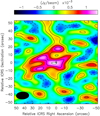 |
Fig. 1. ACA map obtained by integrating the CO(3−2) line emission within −400 < v[km s−1]< 1000. For visualisation purposes, the map has not been divided by the primary beam profile, hence the noise is uniform across the field. Negative contours are shown as dashed curves. Both negative and positive contours are plotted in steps of 1σ starting from ±1σ, with a 1σ = 0.33 mJy beam−1. The phase centre is indicated with a black cross (see coordinates in Table 1) and corresponds to the AGN position. |
The ACA CO(3−2) spectrum is shown in Fig. 2. A Gaussian fit returns a total flux of 8.7 ± 2.6 Jy km s−1, which is a factor of 14 ± 5 higher than estimated by Circosta et al. (2021) for the ISM component. The additional CO(3−2) emission detected by ACA spans a much broader range in line-of-sight velocities than the inner ISM. Although our spectral analysis is limited by the low signal-to-noise (S/N) of the data, by comparing ACA and ALMA spectra extracted from different apertures (see Fig. 2 and additional spectra in Fig. A.3), we infer that: (i) the CO(3−2) emission within rap ≲ 5″ is dominated by a narrow (FWHM ∼ 200 km s−1) line centred at νobs = 107.4 GHz (corresponding to the zCO listed in Table 1). Its peak flux density is maximised in the spectrum extracted from rap = 2.5″ ( mJy), and it remains constant when using bigger extraction areas. (ii) Larger apertures collect significant additional flux due to a second line centred at v ∼ 450 km s−1, a feature that is marginally detected by ALMA even in smaller apertures, but it only becomes dominant at rap > 5″. This component is responsible for the red shift of the main CO(3−2) peak in the low resolution ACA spectra. (iii) For rap > 15″, which are only reliably probed by ACA, we observed – at a spectral resolution of Δvchannel = 160 km s−1 – a very broad line profile extending from v ∼ −400 km s−1 to v ∼ 1000 km s−1 with respect to a central frequency of νobs = 107.4 GHz, with an additional fainter component at v ∼ 1500 km s−1 (see Fig. A.3, bottom panel).
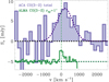 |
Fig. 2. ACA CO(3−2) spectrum extracted from a polygonal region tracing the 2σ contours in Fig. 1 which maximises the S/N (=5). The spectral profile is, however, almost identical to the ACA spectra extracted using circular or elliptical apertures with raperture ≳ 15″ (Fig. A.3, bottom panel). The spectral rms is 2.7 mJy per Δvchannel = 160 km s−1. The best-fit Gaussian parameters are as follows: vcen = 200 ± 100 km s−1, FWHM = 1000 ± 220 km s−1, and Speak = 8.1 ± 1.6 mJy. At the bottom, shifted vertically to facilitate a visual comparison, we show the ALMA CO(3−2) spectrum extracted from a 1″-radius circular aperture. The green dot-dashed line indicates the ALMA CO(3−2) line peak (νobs = 107.4 GHz, zCO = 2.2197). |
The curve of growth in Fig. 3 shows a steady increase in CO(3−2) flux up to rap ≃ 25″, and it plateaus for larger apertures. From this, we infer that the CO halo extends up to r ∼ 200 kpc. This size estimate is consistent with the analysis of the uv visibilities presented in Fig. 4, where the data are modelled using a circular Gaussian function with FWHM = 300 ± 80 kpc, in addition to a point source (the unresolved ISM) which contributes very little to the total flux.
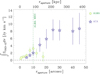 |
Fig. 3. Curve of growth of the CO(3−2) line emission, showing the integrated flux as a function of the radius of the aperture used for spectra extraction. The fluxes were computed through a Gaussian fitting (details in Appendix A.3). Vertical lines correspond to the MRS of the ALMA and ACA data. Error bars include nominal calibration uncertainties (5% for both ALMA and ACA Band 3). Our ALMA data are not reliable for measuring fluxes beyond r > 10″, where aperture dilution effects become severe due to the poor sensitivity to extended and redshifted components. |
4. Discussion and conclusions
Table 3 summarises the CO(3−2) measurements available for cid_346 and its halo: our fiducial ISM value is the one measured by Circosta et al. (2021) at r ≲ 8 kpc, while the fiducial CGM CO(3−2) flux (which includes the ISM contribution) is the one obtained through the Gaussian fit shown in Fig. 2. In the same table, we also report the zeroth-baseline flux extrapolated through the uv visibility fit in Fig. 4, which is consistent, within its (large) error, with the CGM flux measured from the spectrum.
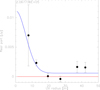 |
Fig. 4. uv plot of the ACA CO(3−2) data integrated between −400 < v[km s−1] < 1000 and binned in uv radii of 8 m. The blue curve is the best-fit with two components: a point source with a flux = 0.8 ± 0.5 Jy km s−1, consistent with the fiducial ISM value, and a circular Gaussian with a flux = 15 ± 11 Jy km s−1 and a FWHM = 35″ ± 10″. |
Summary of CO(3−2) measurements.
Any estimate of molecular gas mass based on a single CO transition is highly uncertain. The uncertainty is even higher in the absence of any (theoretical or observational) constraint on the physical conditions of the gas, which is the case for this newly discovered molecular CGM reservoir around cid_346. An extremely strict lower boundary on  , obtained by simply counting the CO molecules in the J = 3 level in an optically thin regime, is
 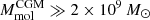 (see Appendix A.4). A more reasonable (but still quite strict) lower limit is
 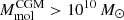 , inferred assuming local thermodynamic equilibrium (LTE). There is however room for up to 1.7 × 10¹² M⊙ of molecular gas in the CGM of cid_346 (upper limit assuming optically thick CO with αCO = 3.6 M⊙ (K km s−1 pc2)−1 and
  , see Appendix A.4). As a comparison, it has been estimated that the CGM of the Milky Way contains a few 109 M⊙ of gas within 75 kpc (Zheng et al. 2019), although a constraint on the molecular phase, as well as on the warm-hot medium, is still missing.
The origin of such a massive molecular CGM reservoir around cid_346 is unclear. Current data (see Appendix A.5) disfavour an over-density of galaxies, contrary to previous (albeit much less extended) detections of molecular halos, all in high-z protoclusters (Ginolfi et al. 2017; Emonts et al. 2016). Therefore, in the absence of better quality data, we set aside the hypothesis that this cold CGM reservoir coincides with a dense environment and thus that it may be the result of gravitational interactions and ram-pressure stripping from satellites.
The moment maps (see Appendix A.6) show complex kinematics, which may be a signature of the direct imprint by AGN-driven outflows, but also of accreting streams. Interestingly, cid_346 is one of the few Type 1 SUPER targets for which high velocity [OIII] λ5007 Å emission, which is a signature of ionised outflows, has been detected as far as ∼3 kpc south-east of the AGN, using SINFONI-AO data (Kakkad et al. 2020). This is also the same direction of the offset of the global ACA CO(3−2) peak with respect to the AGN position (Fig. 1), although we should not over-interpret this result, since the map in Fig. 1 results from an integration of the CO(3−2) emission over a very broad velocity range, and by restricting the velocity range the peak would shift (see e.g. Fig. A.5, left panel). The large line width of the CO emission stemming from the CGM (Fig. 2) is suggestive of outflows, but it may also simply reflect gas assembly within the dark matter halo.
Understanding the presence and survival of molecular gas out to r ∼ 200 kpc is a real puzzle. On the one hand, the fact that the CGM of massive high-z galaxies is shaped by outflows, and, specifically, AGN-driven outflows, is a prediction of models (Nelson et al. 2019; Suresh et al. 2019). On the other hand, whether such outflows can have a direct impact on – or even be responsible for – a molecular CGM reservoir has yet to be proven from a theoretical perspective. It has been shown that clumps of cold gas can survive the entrainment by a hot medium if they are large enough (e.g. Armillotta et al. 2017; Gronke & Oh 2018). This process has, however, never been probed on CGM scales in a cosmological box. In current simulations, even though AGN-driven outflows can have a higher cool (T ∼ 104 K) mass content and thus contribute to seed cold gas on large scales, the outer CGM is still predominantly hot (Nelson et al. 2020). This could be a numerical resolution bias (Hummels et al. 2019) since no current cosmological simulation can track the survival or formation of molecular gas on scales of 100 s of kiloparsecs. Observational evidence that outflows may be linked to extended cold gas CGM reservoirs has been building up, especially in powerful AGN (Cicone et al. 2015; Travascio et al. 2020; Izumi et al. 2021), and cid_346 is the most extraordinary of such cases. However, an in-depth study of such extended cold CGM structures, especially at z ∼ 0, will only be possible with a facility such as the Atacama Large Aperture Submillimeter Telescope (AtLAST, e.g. Klaassen et al. 2020; Cicone et al. 2019).
Measured from the broad, blue-shifted CIV emission component. The spectrum also exhibits a CIV broad absorption line (BAL).
Project number 2018.1.00992.S, PI: C. Harrison.
Acknowledgments
We thank the anonymous referee for the very valuable feedback. CC thanks Padelis P. Papadopoulos for helping us derive sensible limits on the molecular gas masses, and Rolf Güsten for early access to the PI230 instrument. We warmly thank the APEX and ALMA staff for their technical support and their excellent service to the community, especially during the current pandemic. This Letter makes use of the following ACA and ALMA data: ADS/JAO.ALMA#2019.2.00118.S, ADS/JAO.ALMA#2016.1.00798.S. ALMA is a partnership of ESO (representing its member states), NSF (USA) and NINS (Japan), together with NRC (Canada), MOST and ASIAA (Taiwan), and KASI (Republic of Korea), in cooperation with the Republic of Chile. The Joint ALMA Observatory is operated by ESO, AUI/NRAO and NAOJ. This publication is based on data acquired with the Atacama Pathfinder Experiment (APEX). APEX is a collaboration between the Max-Planck-Institut fur Radioastronomie, the European Southern Observatory, and the Onsala Space Observatory. Based on observations collected at the European Organisation for Astronomical Research in the Southern Hemisphere under ESO programmes 098.A-0774(A) and 0101.B-0758(A). GV acknowledges financial support from Premiale 2015 MITiC (PI: B. Garilli). This project has received funding from the European Union’s Horizon 2020 research and innovation programme under grant agreement No 951815.
References
- Armillotta, L., Fraternali, F., Werk, J. K., Prochaska, J. X., & Marinacci, F. 2017, MNRAS, 470, 114 [NASA ADS] [CrossRef] [Google Scholar]
- Arrigoni Battaia, F., Hennawi, J. F., Prochaska, J. X., et al. 2019, MNRAS, 482, 3162 [NASA ADS] [CrossRef] [Google Scholar]
- Bacon, R., Mary, D., Garel, T., et al. 2021, A&A, 647, A107 [NASA ADS] [CrossRef] [EDP Sciences] [Google Scholar]
- Burchett, J. N., Rubin, K. H. R., Prochaska, J. X., et al. 2021, ApJ, 909, 151 [NASA ADS] [CrossRef] [Google Scholar]
- Cai, Z., Cantalupo, S., Prochaska, J. X., et al. 2019, ApJS, 245, 23 [NASA ADS] [CrossRef] [Google Scholar]
- Chen, H. W. 2017, in Outskirts of Distant Galaxies in Absorption, eds. J. H. Knapen, J. C. Lee, & A. Gil de Paz, 434, 291 [CrossRef] [Google Scholar]
- Cicone, C., Maiolino, R., Gallerani, S., et al. 2015, A&A, 574, A14 [NASA ADS] [CrossRef] [EDP Sciences] [Google Scholar]
- Cicone, C., De Breuck, C., Chen, C.-C., et al. 2019, BAAS, 51, 82 [NASA ADS] [Google Scholar]
- Circosta, C., Mainieri, V., Padovani, P., et al. 2018, A&A, 620, A82 [EDP Sciences] [Google Scholar]
- Circosta, C., Mainieri, V., Lamperti, I., et al. 2021, A&A, 646, A96 [EDP Sciences] [Google Scholar]
- Emonts, B. H. C., Lehnert, M. D., Villar-Martín, M., et al. 2016, Science, 354, 1128 [NASA ADS] [CrossRef] [Google Scholar]
- Fossati, M., Fumagalli, M., Gavazzi, G., et al. 2019, MNRAS, 484, 2212 [NASA ADS] [CrossRef] [Google Scholar]
- Fujimoto, S., Silverman, J. D., Bethermin, M., et al. 2020, ApJ, 900, 1 [CrossRef] [Google Scholar]
- Ginolfi, M., Maiolino, R., Nagao, T., et al. 2017, MNRAS, 468, 3468 [CrossRef] [Google Scholar]
- Gronke, M., & Oh, S. P. 2018, MNRAS, 480, L111 [NASA ADS] [CrossRef] [Google Scholar]
- Guo, Y., Maiolino, R., Jiang, L., et al. 2020, ApJ, 898, 26 [Google Scholar]
- Hummels, C. B., Smith, B. D., Hopkins, P. F., et al. 2019, ApJ, 882, 156 [NASA ADS] [CrossRef] [Google Scholar]
- Izumi, T., Matsuoka, Y., Fujimoto, S., et al. 2021, ApJ, 914, 36 [CrossRef] [Google Scholar]
- Kakkad, D., Mainieri, V., Vietri, G., et al. 2020, A&A, 642, A147 [NASA ADS] [CrossRef] [EDP Sciences] [Google Scholar]
- Klaassen, P. D., Mroczkowski, T. K., Cicone, C., et al. 2020, SPIE Conf. Ser., 11445, 114452F [NASA ADS] [Google Scholar]
- Laigle, C., McCracken, H. J., Ilbert, O., et al. 2016, ApJS, 224, 24 [NASA ADS] [CrossRef] [Google Scholar]
- Lamperti, I., Harrison, C. M., Mainieri, V., et al. 2021, A&A, in press, https://doi.org/10.1051/0004-6361/202141363 [Google Scholar]
- McMullin, J. P., Waters, B., Schiebel, D., Young, W., & Golap, K. 2007, in CASA Architecture and Applications, eds. R. A. Shaw, F. Hill, & D. J. Bell, ASP Conf. Ser., 376, 127 [Google Scholar]
- Mehta, V., Scarlata, C., Capak, P., et al. 2018, ApJS, 235, 36 [NASA ADS] [CrossRef] [Google Scholar]
- Nelson, D., Pillepich, A., Springel, V., et al. 2019, MNRAS, 490, 3234 [NASA ADS] [CrossRef] [Google Scholar]
- Nelson, D., Sharma, P., Pillepich, A., et al. 2020, MNRAS, 498, 2391 [NASA ADS] [CrossRef] [Google Scholar]
- Papadopoulos, P. P., van der Werf, P., Xilouris, E., Isaak, K. G., & Gao, Y. 2012, ApJ, 751, 10 [NASA ADS] [CrossRef] [Google Scholar]
- Planck Collaboration VI. 2020, A&A, 641, A6 [NASA ADS] [CrossRef] [EDP Sciences] [Google Scholar]
- Rupke, D. S. N., Coil, A., Geach, J. E., et al. 2019, Nature, 574, 643 [NASA ADS] [CrossRef] [Google Scholar]
- Suresh, J., Nelson, D., Genel, S., Rubin, K. H. R., & Hernquist, L. 2019, MNRAS, 483, 4040 [NASA ADS] [CrossRef] [Google Scholar]
- Travascio, A., Zappacosta, L., Cantalupo, S., et al. 2020, A&A, 635, A157 [NASA ADS] [CrossRef] [EDP Sciences] [Google Scholar]
- Tumlinson, J., Peeples, M. S., & Werk, J. K. 2017, ARA&A, 55, 389 [NASA ADS] [CrossRef] [Google Scholar]
- Valentino, F., Magdis, G. E., Daddi, E., et al. 2018, ApJ, 869, 27 [Google Scholar]
- Valentino, F., Magdis, G. E., Daddi, E., et al. 2020, ApJ, 890, 24 [Google Scholar]
- Veilleux, S., Maiolino, R., Bolatto, A. D., & Aalto, S. 2020, A&ARv, 28, 2 [NASA ADS] [CrossRef] [Google Scholar]
- Vietri, G., Mainieri, V., Kakkad, D., et al. 2020, A&A, 644, A175 [NASA ADS] [CrossRef] [EDP Sciences] [Google Scholar]
- Zheng, Y., Peek, J. E. G., Putman, M. E., & Werk, J. K. 2019, ApJ, 871, 35 [CrossRef] [Google Scholar]
Appendix A: Supplementary material
A.1. ACA non-detection of the continuum
The 3mm continuum flux density measured in cid_346 by Circosta et al. (2021) using ALMA is 0.15 ± 0.04 mJy. Such continuum emission is not detected by ACA. We verified this by using a line-free spectral window (spw17) adjacent to the one containing the CO(3-2) line, but at a lower spectral resolution of Δvchannel = 22 km s−1, which covers observed frequencies between 106.75 and 104.80 GHz. In Figure A.1 we present a collapsed map of the full spw17 range, centred at νobs = 105.796 GHz, which does not show any significant detection. Using this map, we can place an ACA 3σ upper limit on the continuum level of S106 GHz < 0.5 mJy beam−1, which is consistent with the detection by Circosta et al. (2021).
A.2. The APEX [CI](2-1) data
Figure A.2 shows the final APEX PI230 spectrum, obtained by combining all the good quality scans selected from the 2017 and 2018 observing runs, for a total of 16.9 hours of single-polarisation data. The tuning frequency is the redshifted frequency of the [CI](2-1) line (νobs = 251.372 GHz, set to v = 0 km s−1). The CO(7-6) line would be expected at νobs = 250.5363 GHz, thus Δv ∼ 1000 km s−1 redward of the [CI](2-1) line. Neither of the two lines is detected in the APEX data, down to a sensitivity of 7.0 ± 1.2 mJy per Δv = 50 km s−1 channel.
By assuming that the [CI](2-1) and CO(3-2) lines share the same line profile, we can assume FWHM ∼ 1000 km s−1 (see Fig. 2) to place a 3σ upper limit on the [CI](2-1) flux:
![Mathematical equation: $$ \begin{aligned} \mathrm{\int S_{\nu }^{[CI]}dv < 3 \sigma _{rms}}\sqrt{\Delta { v}_{channel}\cdot \mathrm{FWHM}_{\rm [CI]}} \sim 4.7\,\mathrm{Jy\,km\,s^{-1}}, \end{aligned} $$](/articles/aa/full_html/2021/10/aa41611-21/aa41611-21-eq13.gif) (A.1)
(A.1)
which corresponds to }} < 2.4\times10^{10} $](/articles/aa/full_html/2021/10/aa41611-21/aa41611-21-eq14.gif) K km s−1 pc2.
K km s−1 pc2.
A.3. CO(3-2) line spectral fits
In this section we describe, in more detail, the Gaussian fitting procedure used to measure the CO(3-2) fluxes for the curve of growth reported in Fig. 3. A few representative spectra used to compute Fig. 3 are reported in Fig. A.3. The CO(3-2) spectral line profile significantly varies with the aperture used for spectra extraction, and of course it also depends on the S/N of the data and spectral binning applied. The spectra used in this analysis can be divided into three categories, shown in different panels of Fig. A.3.
For small apertures probed by the ALMA data (raperture = 0.6″ − 5″), the CO(3-2) spectrum exhibits a single component, which can be modelled using a Gaussian function. The top panel of Fig. A.3 shows a few examples and reports, in the top-right inset, the best fit to the raperture = 1″ spectrum.
The ALMA spectra extracted using raperture = 7.5″ and 10″ show a clear additional redshifted component at v ∼ 450 − 480 km s−1, brighter than the one at v = 0 km s−1, which is very close to the edge of the ALMA spectral window. These spectra are shown in the middle panel of Fig. A.3.
The ALMA spectra extracted from even larger apertures, with raperture > 10″, are not reliable, even when using the tapered dataset (ALMA-t in Table 1). Indeed, at these scales, the snapshot 1″-resolution ALMA data fail to recover the additional extended flux and the increasingly larger contribution from the redshifted component (due to their limited bandwidth on the red side of the line), and the resulting flux measurement is affected by severe aperture dilution effects. These technical issues are instructively shown by the two ALMA data points at raperture > 10″ in Fig. 3. These fluxes were obtained by fitting the spectra extracted from the ALMA-t cube, using elliptical apertures with semi-major axes of a = 15″, b = 10″ for the data point plotted at raperture = 12.5″, and a = 20″, b = 15″, for the data point plotted at raperture = 17.5″. The resulting flux values fall below the raperture = 10″ value, hence demonstrating the inadequacy of this dataset for probing extended structures.
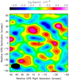 |
Fig. A.1. ACA map showing the non-detection of the 3mm continuum in cid_346, obtained by integrating the emission over the (observed) frequency range νobs ∈ (104.8, 106.75) GHz. Negative and positive contours are plotted in steps of 1σ starting from ±1σ, with a 1σ = 0.18 mJy beam−1. |
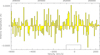 |
Fig. A.2. APEX [CI](2-1) spectrum, with no signs of either the [CI] or the CO emission lines. The window used to mask the line during the baseline fitting is shown. The y-axis units are antenna temperature corrected for atmospheric losses ( |

Apertures with r > 10″ are only reliably probed by the ACA data. The ACA spectra were rebinned to Δvchannel = 160 km s−1 in order to maximise the S/N. All spectra were fitted using a single broad Gaussian component, as shown in the bottom panel of Fig. A.3 (see also Fig. 2). The central velocity of the best-fit Gaussian function varies within the range v ∼ 200 − 300 km s−1 for different apertures, hence robustly displaying a red shift compared to the CO(3-2) emission arising from the inner ISM of cid_346. This is also clearly shown by the comparison between ALMA and ACA spectra in Fig. 2. Although the low S/N of the ACA spectra does not allow us to analyse them at higher spectral resolution, it is likely that the observed global redshift of the CO(3-2) line results from the spectral blending (when using such a large bin size of Δvchannel = 160 km s−1) of the two peaks that are already visible in the ALMA spectra extracted from raperture = 7.5″ and 10″ (middle panel of Fig. A.3). The best-fit FWHM value is ∼1000 km s−1 for all ACA spectral fits. None of these single-Gaussian fits include the additional component centred at v ∼ 1500 km s−1, which is detected at too low of an S/N to be fit separately, but it is consistently present in all the ACA spectra, as shown in the bottom panel of Fig. A.3. We note that we cannot verify whether this component is also present on the smaller ISM scales probed by ALMA because our ALMA data lack the corresponding frequency coverage.
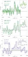 |
Fig. A.3. CO(3-2) spectra extracted using increasingly larger apertures from the primary-beam corrected ALMA and ACA data cubes. The channel widths are 21, 64, 86 km s−1 for the ALMA r = 1″, 2.5″, 4″ spectra (top panel), 86 km s−1 for the ALMA r = 7.5″ and 10″ spectra (middle panel), and 160 km s−1 for the ACA spectra (bottom panel). The aperture radii (or, in the case of elliptical apertures, the major and minor semi-axes) are reported on the plots. The top-right insets in each panel show the Gaussian spectral fits to the ALMA rap = 1″ (top), ALMA rap = 7.5″ (middle), and ACA rap = 15″ (bottom) spectra. |
A.4. Lower and upper limits on 
In the following, we use our fiducial estimate of the CGM CO(3-2) luminosity,  K km s−1 pc2 (Table 3), to place strict lower and upper limits on the CGM molecular gas mass. We treat all of the CO(3-2) emission equally, although the physical conditions in the ISM (inner kiloparsecs) can be different from those on larger scales. In the absence of additional constraints, any assumption would be speculative.
A.4.1. Lower limit on 
A lower boundary for  can be estimated using the optically thin limit. Even in this case, there are several possible routes (see, e.g. Papadopoulos et al. 2012), which are more or less conservative depending on the underlying assumptions. The most minimalist one is to estimate the column density of the molecular gas in the J = 3 level, N3, and from this infer the molecular gas mass assuming only the J = 3 level contribution, that is
 (A.2)
(A.2)
where RCO is the [H2/CO] abundance ratio and μ = 1.36 accounts for the mass in Helium. We have assumed a typical CO abundance [CO/H2] = 10−4 since lower values, for example due to lower metallicities and/or CO-dark H2 gas, would only increase the mass. We stress that Eq. A.2 represents an extremely strict lower limit (hence the ≫ symbol) that is physically unattainable because it does not account for the (significant) contribution to the total column density Ntot due to the CO molecules in the J = 0, 1, 2 levels (or in the J ≥ 4 levels).
To account for the contribution from the other CO energy levels, we can assume local thermodynamic equilibrium (LTE) and so describe the system as a Boltzmann distribution with a single temperature, Tkin. Under this condition, the total column density Ntot can be derived using
 (A.3)
(A.3)
where g3 = 7, ZLTE is the LTE partition function given by ZLTE ≃ 2kBTkin/E1, and the J = 1 and J = 3 state energies are E1/kB = 5.53 K and E3/kB = 33.19 K. Hence, a more reasonable lower limit for the CGM molecular gas mass is as follows:
 (A.4)
(A.4)
Here we have assumed Tkin = 50 K, which corresponds to the lower boundary of the cold neutral medium temperature range.
A.4.2. Upper limit on 
We may estimate an upper limit on  by assuming optically thick CO emission throughout the entire CGM reservoir. Several recent literature studies promote the use of a CO-to-H2 conversion factor of αCO(1 − 0) = 3.6 M⊙ (K km s−1 pc2)−1 (including the Helium correction) for the molecular ISM of z ∼ 2 galaxies (see references in Circosta et al. 2021). Concerning the CO excitation, the literature reports a broad range of
 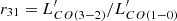 measurements, r31 ∼ 0.5 − 1, at both low and high redshifts. If we assume r31 ∼ 0.5, combined with the αCO(1 − 0) quoted above, we obtain a total molecular gas mass of 1.7 × 10¹² M⊙, which may be considered an upper limit given the premise of optically thick CO emission and the low r31 ratio.
 |
Fig. A.4. Optical and infrared image of the field around cid_346, obtained by combining Subaru and Spitzer photometric data (see Table A.1). The images have been registered to the same astrometric solution, using the one with the best point spread function (z-band) as a reference. Known spectroscopic redshifts from the literature (blue) and photometric redshifts from Laigle et al. (2016) (red) are reported in the image. The red contours show the ACA CO(3-2) 1-3σ level emission from Fig. 1. |
Alternatively, it is possible to convert the APEX [CI](2-1) non-detection into an upper limit on  , by assuming a Carbon excitation temperature Tex and a Carbon abundance XCI = [C]/[H2]. The most updated high-z compilations of [CI](2-1) and [CI](1-0) line measurements by Valentino et al. (2018) and Valentino et al. (2020) provide average values of
 }}/L^\prime_{\mathrm{[CI](1-0)}}= 0.47 $](/articles/aa/full_html/2021/10/aa41611-21/aa41611-21-eq27.gif) (corresponding to Tex = 26 K) and XCI = 1.6 × 10⁻⁵ for the ISM of main sequence galaxies at z > 1. If we adopt these values we obtain Mmol < 9 × 10¹¹ M⊙, which is slightly more stringent than the αCO(1 − 0)-based upper Mmol boundary. However, we note that the APEX single-pointing FoV of 27″ (Table 2) is smaller than the full extent of the CO halo detected by ACA, and an aperture of rap = 15″ contains half of our fiducial CGM CO(3-2) flux (4.2 ± 1.9 Jy km s−1, see Fig. 3), hence the two upper limits are consistent.
(corresponding to Tex = 26 K) and XCI = 1.6 × 10⁻⁵ for the ISM of main sequence galaxies at z > 1. If we adopt these values we obtain Mmol < 9 × 10¹¹ M⊙, which is slightly more stringent than the αCO(1 − 0)-based upper Mmol boundary. However, we note that the APEX single-pointing FoV of 27″ (Table 2) is smaller than the full extent of the CO halo detected by ACA, and an aperture of rap = 15″ contains half of our fiducial CGM CO(3-2) flux (4.2 ± 1.9 Jy km s−1, see Fig. 3), hence the two upper limits are consistent.
Finally, we note that some caution must be taken when comparing these mass estimates with the previous molecular CGM detections by Ginolfi et al. (2017) and Emonts et al. (2016). Indeed, these studies used very high αCO(1 − 0) values of αCO(1 − 0) = 10 and αCO(1 − 0) = 4 M⊙ (K km s−1 pc2)−1, respectively.
A.5. Continuum sources in the field
Figure A.4 displays the ACA CO(3-2) contours overlaid on the optical and infrared image of the field, obtained by combining photometric data from the Subaru and Spitzer telescopes. The central wavelength (λcen) and FWHM of the photometric filters, as well as the point spread function (PSF) and sensitivity of the images are listed in Table A.1. Figure A.4 shows that the ACA CO peaks do not coincide with any known optical or infrared source. The galaxies with a photometric or spectroscopic redshift measurement that lie close to the CO contours have redshifts that are not consistent with the range inferred from the CO data of z ∼ 2.215 − 2.230. In addition, sensitive ALMA Band 7 continuum observations5 do not show any dust continuum emitters besides cid_346 within a FoV of 16″.
Furthermore, there is no clear indication that cid_346 is in a galaxy pair or in a merging state. The target appears as a point source both in the COSMOS HST-Advanced Camera for Surveys data (rest-frame UV, PSF = 0.12″) and in the UltraVista near-infrared data (seeing-limited, FWHM ≃ 0.78″) (Laigle et al. 2016). Even at longer wavelengths, cid_346 does not show close companions. Its rest frame 260-μm continuum emission (870μm observed frame) was imaged at ∼2 kpc resolution with a very high S/N (∼29, Lamperti et al. 2021) and resolved into a Gaussian distribution with half-light radius Re = 1.81 kpc and a possible additional central point source (a compact starburst or the AGN) contributing ∼13% to the flux.
A.6. CO(3-2) moment maps
Figure A.5 shows the ACA CO(3-2) moment maps. These were produced with the task immoments in CASA by selecting the velocity range v ∈ [ − 300, 300] km s−1 and masking pixels below a flux threshold of 0.04 Jy beam−1 km s−1. Since it was produced by applying a flux and a velocity threshold, the moment 0 map (left panel of Fig. A.5) is biased against faint and high-velocity emission, and it is shown only for completeness. We refer to Fig. 1 for an unbiased, total CO(3-2) flux map.
The velocity map (middle panel of Fig. A.5) does not display a regular velocity gradient. However, about 15″ north-east of the AGN position, it is possible to identify an extended region of predominantly redshifted emission with 150 ≲ v[km s−1] < 200, and an average velocity dispersion of σv ∼ 120 km s−1. Almost symmetrically, ∼15″ south-west of the AGN, the CO(3-2) is mostly blueshifted, with −250 < v[km s−1] ≲ −200 and an overall low velocity dispersion of σv < 50 km s−1. In the central portion of the field, just south-west of the redshifted area, the moment 2 map shows a stripe of high-σv CO emission extending towards the east, with σv ≳ 200 km s−1. Other clear distinctive features of the moment maps are two spots of redshifted CO emission about 20″ west of the AGN, offset in declination by Δδ ∼ +10″ and Δδ ∼ −10″, respectively, and two regions of high σv ≳ 200 km s−1 between them.
Interestingly, the velocity dispersion peaks are not centred on cid_346. This may favour accreting streams over the AGN-outflow interpretation for explaining the kinematics of the molecular CGM, since in the outflow scenario one would expect the σv peak to coincide with the AGN position. However, we caution against an over-intepretation of Fig. A.5 since the very large beam of ACA would dilute any kinematic signature of kiloparsec-scale outflows. In fact, the ACA resolution of 80 kpc is much larger than any ISM structure (disk, ring, or outflow) ever observed in molecular tracers. At this resolution, even the two largest detections of molecular CGM reservoirs prior to this work, that is the Spiderweb protocluster (70 kpc, Emonts et al. 2016) and Candels-5001 (40 kpc, Ginolfi et al. 2017), would be unresolved. Therefore, the kinematic features resolved by ACA around cid_346, shown in Figure A.5, cannot be compared to anything known. Due to the poor resolution and low S/N of the data, none of these features can be studied in detail.
Description of the RGB data used in Fig. A.4.
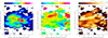 |
Fig. A.5. ACA CO(3-2) moment maps, produced by selecting the velocity range to −300 < v[km s−1]< 300. The left panel shows the zeroth moment map (flux), with contours at [0.2, 0.3, 0.4, 0.5, 0.6] Jy beam−1 km s−1; the middle panel shows the first moment map (velocity), with contours corresponding to [-250, -150, -50, 50, 150, 250] km s−1; the right panel shows the second moment map (σv), with contours at [50, 100, 150, 200, 250] km s−1. The black cross indicates the AGN position, whose coordinates are reported in Table 1. |
All Tables
All Figures
|
Fig. 1. ACA map obtained by integrating the CO(3−2) line emission within −400 < v[km s−1]< 1000. For visualisation purposes, the map has not been divided by the primary beam profile, hence the noise is uniform across the field. Negative contours are shown as dashed curves. Both negative and positive contours are plotted in steps of 1σ starting from ±1σ, with a 1σ = 0.33 mJy beam−1. The phase centre is indicated with a black cross (see coordinates in Table 1) and corresponds to the AGN position. |
| In the text | |
|
Fig. 2. ACA CO(3−2) spectrum extracted from a polygonal region tracing the 2σ contours in Fig. 1 which maximises the S/N (=5). The spectral profile is, however, almost identical to the ACA spectra extracted using circular or elliptical apertures with raperture ≳ 15″ (Fig. A.3, bottom panel). The spectral rms is 2.7 mJy per Δvchannel = 160 km s−1. The best-fit Gaussian parameters are as follows: vcen = 200 ± 100 km s−1, FWHM = 1000 ± 220 km s−1, and Speak = 8.1 ± 1.6 mJy. At the bottom, shifted vertically to facilitate a visual comparison, we show the ALMA CO(3−2) spectrum extracted from a 1″-radius circular aperture. The green dot-dashed line indicates the ALMA CO(3−2) line peak (νobs = 107.4 GHz, zCO = 2.2197). |
| In the text | |
|
Fig. 3. Curve of growth of the CO(3−2) line emission, showing the integrated flux as a function of the radius of the aperture used for spectra extraction. The fluxes were computed through a Gaussian fitting (details in Appendix A.3). Vertical lines correspond to the MRS of the ALMA and ACA data. Error bars include nominal calibration uncertainties (5% for both ALMA and ACA Band 3). Our ALMA data are not reliable for measuring fluxes beyond r > 10″, where aperture dilution effects become severe due to the poor sensitivity to extended and redshifted components. |
| In the text | |
|
Fig. 4. uv plot of the ACA CO(3−2) data integrated between −400 < v[km s−1] < 1000 and binned in uv radii of 8 m. The blue curve is the best-fit with two components: a point source with a flux = 0.8 ± 0.5 Jy km s−1, consistent with the fiducial ISM value, and a circular Gaussian with a flux = 15 ± 11 Jy km s−1 and a FWHM = 35″ ± 10″. |
| In the text | |
|
Fig. A.1. ACA map showing the non-detection of the 3mm continuum in cid_346, obtained by integrating the emission over the (observed) frequency range νobs ∈ (104.8, 106.75) GHz. Negative and positive contours are plotted in steps of 1σ starting from ±1σ, with a 1σ = 0.18 mJy beam−1. |
| In the text | |
|
Fig. A.2. APEX [CI](2-1) spectrum, with no signs of either the [CI] or the CO emission lines. The window used to mask the line during the baseline fitting is shown. The y-axis units are antenna temperature corrected for atmospheric losses ( |
| In the text | |
|
Fig. A.3. CO(3-2) spectra extracted using increasingly larger apertures from the primary-beam corrected ALMA and ACA data cubes. The channel widths are 21, 64, 86 km s−1 for the ALMA r = 1″, 2.5″, 4″ spectra (top panel), 86 km s−1 for the ALMA r = 7.5″ and 10″ spectra (middle panel), and 160 km s−1 for the ACA spectra (bottom panel). The aperture radii (or, in the case of elliptical apertures, the major and minor semi-axes) are reported on the plots. The top-right insets in each panel show the Gaussian spectral fits to the ALMA rap = 1″ (top), ALMA rap = 7.5″ (middle), and ACA rap = 15″ (bottom) spectra. |
| In the text | |
|
Fig. A.4. Optical and infrared image of the field around cid_346, obtained by combining Subaru and Spitzer photometric data (see Table A.1). The images have been registered to the same astrometric solution, using the one with the best point spread function (z-band) as a reference. Known spectroscopic redshifts from the literature (blue) and photometric redshifts from Laigle et al. (2016) (red) are reported in the image. The red contours show the ACA CO(3-2) 1-3σ level emission from Fig. 1. |
| In the text | |
|
Fig. A.5. ACA CO(3-2) moment maps, produced by selecting the velocity range to −300 < v[km s−1]< 300. The left panel shows the zeroth moment map (flux), with contours at [0.2, 0.3, 0.4, 0.5, 0.6] Jy beam−1 km s−1; the middle panel shows the first moment map (velocity), with contours corresponding to [-250, -150, -50, 50, 150, 250] km s−1; the right panel shows the second moment map (σv), with contours at [50, 100, 150, 200, 250] km s−1. The black cross indicates the AGN position, whose coordinates are reported in Table 1. |
| In the text | |
Current usage metrics show cumulative count of Article Views (full-text article views including HTML views, PDF and ePub downloads, according to the available data) and Abstracts Views on Vision4Press platform.
Data correspond to usage on the plateform after 2015. The current usage metrics is available 48-96 hours after online publication and is updated daily on week days.
Initial download of the metrics may take a while.