| Issue |
A&A
Volume 654, October 2021
|
|
|---|---|---|
| Article Number | A131 | |
| Number of page(s) | 12 | |
| Section | Stellar structure and evolution | |
| DOI | https://doi.org/10.1051/0004-6361/202141378 | |
| Published online | 22 October 2021 | |
Detecting the intrinsic X-ray emission from the O-type donor star and the residual accretion in a supergiant fast X-ray transient in its faintest state⋆
1
INAF, Istituto di Astrofisica Spaziale e Fisica Cosmica, Via A. Corti 12, 20133 Milano, Italy
e-mail: This email address is being protected from spambots. You need JavaScript enabled to view it.
2
Sternberg Astronomical Institute, Lomonosov Moscow State University, Universitetskij pr. 13, 119234 Moscow, Russia
3
Kazan Federal University, Kremlyovskaya 18, 420008 Kazan, Russia
4
Institute for Physics and Astronomy, University Potsdam, 14476 Potsdam, Germany
5
Scuola Universitaria Superiore IUSS Pavia, Piazza della Vittoria 15, 27100 Pavia, Italy
6
INFN, Sezione di Pavia, Via A. Bassi 6, 27100 Pavia, Italy
Received:
25
May
2021
Accepted:
22
June
2021
Abstract
We report on the results of an XMM–Newton observation of the supergiant fast X-ray transient (SFXT) IGR J08408-4503 performed in June 2020. The source is composed of a compact object (likely a neutron star) orbiting around an O8.5Ib-II(f)p star, LM Vel. The X-ray light curve shows a very low level of emission, punctuated by a single, faint flare. We analysed spectra measured during the flare and during quiescence. The quiescent state shows a continuum spectrum that is well deconvolved to three spectral models: two components are from a collisionally ionized plasma (with temperatures of kT1 = 0.24 keV and kT2 = 0.76 keV), together with a power-law model (photon index, Γ, of ∼2.55), dominating above ∼2 keV. The X-ray flux emitted at this lowest level is 3.2 × 10⁻¹³ erg cm−2 s−1 (0.5–10 keV, corrected for the interstellar absorption), implying an X-ray luminosity of 1.85 × 1032 erg s−1 (at 2.2 kpc). The two-temperature collisionally ionized plasma is intrinsic to the stellar wind of the donor star, while the power-law can be interpreted as emission due to residual, low-level accretion onto the compact object. The X-ray luminosity contributed by the power-law component only, in the lowest state, is (4.8 ± 1.4)×1031 erg s−1, which is the lowest quiescent luminosity detected from the compact object in an SFXT. Thanks to this very faint X-ray state caught by XMM–Newton, X-ray emission from the wind of the donor star LM Vel could be well-established and studied in detail for the first time, along with a very low level of accretion onto the compact object. The residual accretion rate onto the compact object in IGR J08408-4503 can be interpreted as the Bohm diffusion of (possibly magnetized) plasma entering the neutron star magnetosphere at low Bondi capture rates from the supergiant donor wind at the quasi-spherical, radiation-driven settling accretion stage.
Key words: stars: neutron / supergiants / X-rays: binaries / stars: individual: IGR J08408-4503 / stars: individual: HD 74194 / stars: individual: LM Vel
Based on observations (ObsID 0861460101) obtained with XMM-Newton, an ESA science mission with instruments and contributions directly funded by ESA member states and NASA.
© ESO 2021
1. Introduction
IGR J08408-4503 is a transient X-ray source discovered during an outburst in 2006 thanks to observations performed by the INTEGRAL satellite (Götz et al. 2006). Not long after, the analysis of INTEGRAL archival data revealed an earlier outburst that occurred in 2003 (Mereghetti et al. 2006), and thus unveiled a recurrent, bright flaring X-ray activity of the source. IGR J08408-4503 was associated with the O-type supergiant LM Vel (also known as HD 74194; Götz et al. 2006; Masetti et al. 2006; Barba et al. 2006; Kennea & Campana 2006) leading to its classification as a supergiant fast X-ray transient (SFXT), and thus a new type of high-mass X-ray binary (HMXBs; Kretschmar et al. 2019) discovered during the INTEGRAL monitoring of the Galactic plane (Sguera et al. 2005, 2006; Negueruela et al. 2006).
Supergiant fast X-ray transients (SFXTs) are detected by INTEGRAL during bright flares lasting a quite short interval of time (∼1–2 ks) and, usually, reaching peak luminosities of 1036–1037 erg s−1 (see Sidoli 2017; Sidoli & Paizis 2018 for reviews). The SFXT flares can be part of rare (less than 5% of the time, Sidoli & Paizis 2018) longer outbursts, with a duration of a few days (Romano et al. 2007; Rampy et al. 2009; Sidoli et al. 2016).
The monitoring campaigns with the Neil GehrelsSwift satellite have shown that the most frequent X-ray state in SFXTs is at luminosities below a few ×1034 erg s−1 (Sidoli et al. 2008; Romano 2015), down to X-ray luminosities of ∼1032 erg s−1 in some members of the class (in’t Zand 2005; Bozzo et al. 2010; Sidoli et al. 2010). This huge range of X-ray variability is a characterizing property of the SFXT class (an updated list of the dynamic range of X-ray fluxes and duty cycles in SFXTs, compared with other types of HMXBs can be found in Sidoli & Paizis 2018). Nowadays, the SFXT class has about twenty confirmed members, plus a similar number of candidates still missing optical or infrared (IR) identifications.
In persistent HMXBs with supergiant massive donor stars, the high X-ray luminosity is sustained by the accretion of stellar wind material onto the compact object, usually a neutron star (NS). The massive star winds are quite stationary and uniform when averaged over years (Lamers & Cassinelli 1999). However, on shorter timescales (days to hours), the non-stationary processes, such as shocks, are operating in stellar winds (Feldmeier et al. 1997). Moreover, the large-scale structures co-rotating with the star, as well as the small-scale inhomogeneities (often referred to as clumps), are ubiquitous in radiatively driven winds (Puls et al. 2008; Massa et al. 2019; Vink & Sander 2021).
SFXTs are HMXBs with a compact object orbiting an OB supergiant companion, but they behave in a completely different way. The physical mechanism responsible for the SFXT phenomenology continues to be debated; the quasi-spherical settling accretion regime (Shakura et al. 2012, 2014), the propeller mechanism, and the magnetic barrier (Grebenev & Sunyaev 2007; Bozzo et al. 2008) are the most discussed theoretical explanations to date. These mechanisms are able to reduce the accretion of wind material onto the NS most of the time. Nevertheless, the issue remains controversial because in almost all SFXTs the important properties of the donor star and of the compact object are unknown.
So far, only a few systems have been spectroscopically observed at optical, IR, and ultraviolet (UV) wavelengths and analyzed using modern stellar atmosphere models required to determine characteristics of the donor’s wind (e.g., Giménez-García et al. 2016; Hainich et al. 2020). These studies showed that the winds of donor stars do not drastically differ from their single-star counterparts: the winds are clumped and have usual mass-loss rates and wind velocities. However, the radiation from an accreting compact object located near the donor star has a noticeable effect on the outer stellar atmosphere and can change the wind ionization and acceleration (Sander 2019). All early-type OB supergiant stars are intrinsic X-ray sources (Berghoefer et al. 1997) emitting soft X-rays at LX ∼ 1032 erg s−1. Therefore, it might be expected that the intrinsic X-ray emission from stellar winds could also be detected in HMXBs if X-rays produced by accretion do not significantly outshine radiation from the donor’s wind.
The orbital geometry in SFXTs remains unclear; while orbital periods have been measured in about a half of the systems (from the periodic modulation of their X-ray long-term light curve), the eccentricity is largely unknown (see the reviews by Walter et al. 2015; Martínez-Núñez et al. 2017; Sidoli & Paizis 2018, and Kretschmar et al. 2019 for updated lists of their orbital periods). Among all SFXTs, the subject of this study, IGR J08408-4503, provides one of the most important laboratories for investigating the physics governing SFXT phenomenology. It is the only SFXT with a well-determined orbital geometry: its orbit is very eccentric, e = 0.63 ± 0.03, with 9.5436 ± 0.0002 d orbital period (Gamen et al. 2015). The distance is also well known: according to Gaia Early Data Release 3 (Gaia Collaboration 2021), it is located at a distance of  kpc (Bailer-Jones et al. 2021).
IGR J08408-4503 has an extremely low-duty cycle. INTEGRAL data show that it undergoes bright (i.e., above a flux of ∼3 × 10⁻¹⁰ erg cm−2 s−1 in the energy range 18–50 keV) X-ray flares for only 0.09% of the time (Sidoli & Paizis 2018). The outbursts occurred in a broad range of orbital phases (Δϕ ≈ ±0.15) around periastron (a collection of bright X-ray flares is reported by Gamen et al. 2015 and Ducci et al. 2019). Nevertheless, it is important to remark that the passage at periastron does not necessarily trigger an outburst; this is clear from a very long observation performed with Suzaku around periastron when the X-ray luminosity remained in the range 1032–1033 erg s−1 (Sidoli et al. 2010). IGR J08408-4503 spends about 68% of the time with an X-ray luminosity below 1.1 × 1033 erg s−1 in the 2–10 keV energy band (Romano 2015). X-ray pulsations have not been detected in IGR J08408-4503; therefore, the nature of the compact object is not firmly established. Nevertheless, an NS is usually assumed (as in other SFXTs; Sidoli 2017), since the X-ray spectrum in outburst resembles the spectra of accreting pulsars in HMXBs (Götz et al. 2007; Sidoli et al. 2009; Romano et al. 2009).
As for the whole SFXT class, the physical mechanism driving the IGR J08408-4503 behavior is heavily debated; previous literature investigated the supergiant clumpy winds (Hainich et al. 2020), the role played by the eccentric orbit (Bozzo et al. 2021), and the possibility of an accretion disk formation fed by Roche-lobe overflow (Ducci et al. 2019).
In this paper, we report the XMM–Newton observation of IGR J08408-4503 performed in June 2020 (Sect. 2) around the orbital phase ∼0.65, just after the apastron passage, catching this SFXT in a very low luminosity state. The timing and spectral analysis are reported in Sects. 3 and 4, while in Sect. 4.1 we interpret the lowest X-ray emission in terms of a twofold contribution: X-rays from the donor wind and residual accretion onto the compact object, which is the lowest luminosity state ever detected from a SFXT. The comparison with previous observations of faint X-ray emission in IGR J08408-4503 is outlined in Sect. 5. The physical picture explaining the very low accretion rate observed by XMM–Newton is discussed in Sects. 6.1 and 6.2. Finally, Sect. 7 features our conclusions.
2. Observation and data reduction
IGR J08408-4503 was observed by XMM–Newton (Jansen et al. 2001) in June 2020, with a net exposure time of ∼47 ks (details of the EPIC exposures are reported in Table 1). All EPIC cameras (Strüder et al. 2001; Turner et al. 2001) operated in full-frame mode and using the medium filter.
Summary of the XMM–Newton observation targeted on IGR J08408-4503.
Data (Obs.ID 0861460101) were reprocessed using version 18 of the XMM–Newton Science Analysis Software (SAS), adopting standard procedures. The response and ancillary matrices were generated with rmfgen and arfgen available in the SAS. A part of the exposure time at the start of the observation that was affected by the high background was excluded from the extraction of all source products.
Source light curves and spectra were extracted from circular regions centered on the source emission, with a 30″ radius for the pn and 60″ for the two MOS, and selecting pattern from 0 to 4 (EPIC pn), and from 0 to 12 (MOS). Background spectra were obtained from similar size regions offset from the source position. IGR J08408-4503 was observed at a very low state (in Table 1, last column, the time-averaged EPIC net count rates are listed), too faint for a meaningful spectroscopy with the Reflection Grating Spectrometer (den Herder et al. 2001).
EPIC spectra were simultaneously fit in the 0.3–12 keV energy range using XSPEC (version 12.10.1; Arnaud 1996), including cross-calibration constants to take into account calibration uncertainties. All fluxes were estimated in the 0.5–10 keV range, for consistency with previous literature. When fitting the spectra, the absorption model TBABS was adopted, assuming the photoelectric absorption cross sections of Verner et al. (1996) and the interstellar abundances of Wilms et al. (2000). The spectra were rebinned to have at least 25 counts per bin, to apply the χ2 statistics. All uncertainties in the spectral analysis are given at 90% confidence level, for one interesting parameter. The uncertainty on the unabsorbed X-ray fluxes have been obtained using CFLUX in XSPEC. All luminosities were calculated assuming a source distance of 2.2 kpc.
3. Temporal analysis
The source was caught by XMM–Newton in a very low emission state. The light curves in two energy ranges (above and below 2 keV) are shown in Fig. 1, together with their hardness ratio. A single faint source flare was observed, after about 12 ks from the beginning of the EPIC pn exposure. Harder emission is evident during the flare.
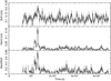 |
Fig. 1. Source light curve (EPIC pn, not background subtracted, bin time = 256 s) in two energy ranges (Soft = 0.3–2 keV, Hard = 2–12 keV), together with their hardness ratio. The first ∼6000 s of the observation have been excluded because of high background level. |
We searched the data for the presence of periodic modulations by means of a Fourier transform. Since we ascertained that both the source flare around 12 ks and the data gap produced by its removal cause strong non-Poissonian noise in the power density spectrum, we only used the part of the observation after the flare, for an exposure of about 29.3 ks. We did not find any candidate signal and set an upper limit on the pulsed fraction (defined as the semi-amplitude of the sinusoidal profile divided by the mean count rate) of ≈30% for periods from ∼0.15 to 15 000 s for a sinusoidal modulation (in the 1–10 keV energy range; we only used the EPIC pn data below 5.4 s and the combined pn and MOS data above). No other structures, such as quasi-periodic oscillation features, are discernible in the same range in the Fourier power-density spectra.
4. Spectroscopy
During the flare event, the source hardness ratio increased (Fig. 1, bottom panel), prompting us to perform spectroscopic analyses at three different states of the source flux selected using the EPIC pn light curve (Fig. 2). We extracted spectra from the following intervals: below 0.05 count s−1 (lowest state, Sect. 4.1), between 0.05 and 0.1 count s−1 (intermediate state, Sect. 4.2), and above 0.1 count s−1 (Sect. 4.3).
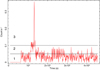 |
Fig. 2. Source light curve (EPIC pn, 1–10 keV, not background subtracted, bin time = 100 s), where the horizontal lines mark the three count rate intervals adopted for the intensity selected spectroscopy: interval 1 (lowest state), 2 (intermediate state), and 3 (the faint flare). |
4.1. The lowest state
The spectrum extracted from the data accumulated during the lowest state could not be fit by any single spectroscopic model; for example, in Fig. 3 we show the residuals when a single, absorbed power-law model is adopted. Therefore, as a next step, we fit the observed spectrum with various types of two-component models, each of them providing statistically good fits. The two-component models we considered are combinations of a thermal emission (a black body or a collisionally ionized plasma model such as APEC), with a second component, either a hotter thermal model or a power-law.
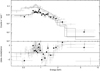 |
Fig. 3. EPIC spectra extracted from the lowest state, fit by a single absorbed power-law model. Upper panel: count spectra, lower panel: residuals with respect to the model in terms of standard deviation. The meaning of the symbols is the following: crosses, empty circles, and solid squares mark the EPIC pn, MOS1, and MOS2 spectra, respectively. |
In the appendix, the spectral parameters obtained with six different models are shown in Table A.1. We note that in just one case (Model 6 in Table A.1), two absorption components were needed to obtain an acceptable fit: the additional one was provided by a partial covering absorption model (PCFABS in XSPEC). Since from a statistical point of view all six models provide equally good descriptions of the spectrum at the lowest state, to choose the realistic model we need to take into account the nature and the properties of the source.
The donor star, LM Vel, has the O8.5Ib-II(f)p spectral type (Sota et al. 2014), and therefore, as is the case of other OB supergiants, it should be an intrinsic source of X-rays (Harnden et al. 1979; Cassinelli et al. 1981). The commonly accepted explanation attributes X-rays to the radiatively driven winds of these stars. The wind instabilities lead to shocks and the consequent heating of the part of wind matter to X-ray-emitting temperatures (Feldmeier et al. 1997). The shocked wind plasma emits thermal X-rays. While this mechanism may not be as effective as previously thought (Steinberg & Metzger 2018), observationally the X-ray properties of OB supergiants are well established (e.g., Berghoefer et al. 1997; Nazé 2009; Oskinova 2016). The typical X-ray spectrum of an O supergiant star is described by a multi-temperature, optically thin plasma model (e.g., APEC). In case of the two-temperature models, the temperature components kT1 ≈ 0.2–0.3 keV and kT2 ≈ 0.7–0.8 keV are typically found (e.g., Rauw et al. 2015; Huenemoerder et al. 2020).
Nebot Gómez-Morán & Oskinova (2018) investigated the dependence of X-ray properties of O-stars on stellar and wind parameters. They show that the X-ray luminosity of O-type supergiants is log(LX[erg s−1]) ≈ 32.7 ± 0.2 and that it does not correlate with stellar bolometric luminosity. Thus, LM Vel is by itself an intrinsic source of X-rays. Indeed, the well-studied star ζ Ori has a similar spectral type, O9.7Ib. Its X-ray luminosity is log(LX[erg s−1]) ≈ 32.8 and the X-ray spectrum is that of thermal coronal plasma with 0.2 keV and 0.8 keV temperature components. Another star with a similar spectral type, HD 149404 (O8.5Iab) also has log(LX[erg s−1]) ≈ 32.7. Brief analysis of its archival XMM-Newton observations shows that its X-ray spectrum could be well described by a two-temperature APEC model with ≈0.2 keV and ≈0.8 keV components.
In addition, somewhat hotter plasma components are, sometimes, measured in the spectra of OB+OB binaries where stellar winds collide with each other (Rauw & Nazé 2016). However, to the best of our knowledge, nonthermal X-ray radiation described by a power-law spectrum has not been observed either in single or binary OB supergiants with colliding winds.
None of the two-component models reported in Table A.1 are typical for an X-ray spectrum of a single OB supergiant. In particular, the two-temperature APEC model (Model 3) would be favored, but it displays a plasma component with a temperature of ∼3 keV, which is much hotter than that typically deduced from the X-ray spectroscopy of these stars. Another issue with the two APEC models is the resulting low absorbing column density, NH. The reddening toward LM Vel is well established from the analysis of the UV spectra, E(B − V) = 0.44 (Hainich et al. 2020). Using RV = 3.1, the extinction toward LM Vel is AV = 1.364 mag. The conversion between extinction and hydrogen-equivalent absorbing column density has been investigated by several authors, sometimes with significantly different results (e.g., Bohlin et al. 1978; Predehl & Schmitt 1995; Vuong et al. 2003; Gudennavar et al. 2012; Liszt 2014; Zhu et al. 2017; Foight et al. 2016). We used the relation found by Foight et al. (2016), NH = 2.87 × 10²¹AV cm−2 mag−1, to be consistent with our overall spectral analysis, since these authors adopted the interstellar abundances according to Wilms et al. (2000). This implies a value of NH = 3.9 × 1021 cm−2 toward LM Vel. Therefore, we fixed the absorbing column density to this value during the fitting with the two APEC models, but the resulting fit was poor, with positive residuals below 1 keV.
On the basis of these considerations, in the next step we consider three-component models. We added a third continuum component to the two APEC models: either a third APEC model or a power-law (see Table 2 for the spectral parameters resulting from these two models). Since the double-temperature APEC plus the power-law continuum resulted in a better description of the spectrum (Model 2 in Table 2), this is our final model describing X-ray spectrum of IGR J08408-4503 during its lowest state (Fig. 4).
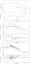 |
Fig. 4. Best fit of the IGR J08408-4503 spectra extracted during the lowest luminosity state (lower panel; Model 2 in Table 2), the intermediate state (middle panel; Model C in Table 3), and the faint flare (upper panel; Model B in Table 4). The counts spectra are plotted together with the residuals in units of standard deviation. The meaning of the symbols are the same as in Fig. 3. |
Spectroscopy of the lowest luminosity state (EPIC pn, MOS1, and MOS2), fixing the absorption to the optical value toward LM Vel (NH = 3.9 × 1021 cm−2).
The physical interpretation of our favorite model is straightforward. The luminosity and the temperatures of the thermal APEC model components are consistent with the expectations from an intrinsic X-ray emission of the O-type supergiant donor star. We interpret the power-law model component as emission produced by low-level residual accretion onto the NS. The power-law flux is ∼8 × 10⁻¹⁴ erg cm−2 s−1 (0.5–10 keV, corrected for the absorption), implying a power-law X-ray luminosity of (4.8 ± 1.4)×1031 erg s−1 (this uncertainty accounts for the uncertainty on the flux only, not on the source distance).
We remark that, even fixing the absorbing column density to the lowest value toward LM Vel (NH = 2.2 × 1021 cm−2, resulting from the relation NH = 5 × 10²¹E(B − V) cm−2 mag−1; Vuong et al. 2003), our conclusions do not change: the resulting temperatures of the two thermal components remain the same (within the uncertainties), as well as the photon index and power-law-emitted flux. The only parameter that would be significantly affected is the normalization of the softest thermal model: it would decrease to one third of the value reported in Table 2, but still be consistent with X-ray emission from the supergiant wind.
4.2. The intermediate state
We have investigated the spectra extracted from the intermediate state (marked by number 2 in Fig. 2), by adopting the same best-fit continuum found in the spectroscopy of the lowest X-ray emission: two thermal plasma models plus a power-law (Model 2 in Table 2). Since the two thermal models are consistent with emission from the wind of the companion star, we fixed their parameters to the best fit found in the spectroscopy of the lowest luminosity state. The power-law model parameters were allowed to vary during the fit, adopting three versions of this continuum model, as reported in Table 3: in Model A, only the parameters of the power-law are left free to vary; in Model B, the absorbing column density of the overall continuum is also allowed to vary (this is because a larger absorption than what is predicted from the optical extinction toward the donor star can sometimes be observed in HMXBs); in Model C, an additional absorption of the power-law model only is included, while the absorbing column density of the overall continuum is fixed to the value of LM Vel (Fig. 4).
The intermediate state can be explained with an increased flux from the power-law component only, the contribution of which increases from 25% of the total unabasorbed 0.5–10 keV radiation in the lowest state to ∼60% in the intermediate state. The total X-ray luminosity reaches ∼3 − 4 × 1032 erg s−1 during the intermediate state.
4.3. The faint X-ray flare
Adopting the same procedure used in the spectral analysis of the intermediate state, we fit the spectra extracted from the faint flare (interval 3 in Fig. 2) with a continuum composed of two thermal plasma models together with a power-law. The spectral results are listed in Table 4. The meaning of the three models is the same as outlined in the previous section (Sect. 4.2). The spectrum fitted with one of these models is shown in Fig. 4.
During the faint flare, the contributed flux from the power-law component is almost 90% of the total unabsorbed 0.5–10 keV flux. The power-law appears harder with the increasing X-ray intensity (from the lowest state to the faint flare). The total X-ray luminosity reaches 1033 erg s−1 in this state.
5. Comparison of the lowest state with previous X-ray observations
IGR J08408-4503 was previously observed in a low state by XMM–Newton in 2007 (Bozzo et al. 2010) and by Suzaku in 2009 (Sidoli et al. 2010). These observations were performed at different orbital phases (ϕ = 0.66–0.71 and ϕ = 0.82–0.97, respectively) and with a higher average X-ray flux than observed in 2020.
In previous sections, we demonstrate that a good deconvolution of the continuum spectrum, also motivated by the known physical properties of the source, is composed of two thermal plasma models plus a power law. Since the two thermal models are compatible with X-ray emission from the wind of the supergiant donor, they should also be present in previous XMM–Newton and Suzaku observation with the same parameters (assuming no long-term variability from the stellar wind in LM Vel). We can ascribe the (variable) power-law component to emission from the compact object. To investigate the hardness and the intensity of the power-law emission during the lowest state in previous observations, we selected the lowest states emission also in 2007 and in 2009.
In particular, we have applied the same intensity filter for the lowest state of the 2020 observation to the 2007 XMM–Newton observation, meaning an EPIC pn source count rate lower than 0.05 count s−1 (the reader can refer to Sidoli et al. 2010 and Bozzo et al. 2010 for more details on this XMM–Newton observation). The two MOS spectra were extracted using the same good time intervals, obtaining the 2007 XMM–Newton spectra reported in Fig. 5 (right panel). There, we show the residuals with respect to the best fit of the lowest intensity observed in 2020: while the soft part is well accounted for by the two thermal models (confirming it is a steady spectral component), the harder region of the spectrum shows an excess with respect to the power-law model fitting the 2020 X-ray emission. When left free to vary, the best-fit power-law component of the 2007 XMM–Newton observation shows a photon index of  and an unabsorbed power-law flux of UFpow = (1.34 ± 0.26)×10−13 erg cm−2 s−1 (0.5–10 keV; reduced χ2 = 1.064 for 62 degrees of freedom; d.o.f.).
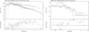 |
Fig. 5. Comparison of Suzaku (on the left) and XMM–Newton observations performed in 2007 (on the right) with the best fit of the lowest luminosity state observed in 2020 with XMM–Newton. Residuals are reported in the lower panels in units of standard deviations. The meaning of the symbols in the right panel is the following: crosses, empty circles, and solid squares mark the EPIC pn, MOS1, and MOS2 spectra, respectively. Clearly, past observations caught IGR J08408-4503 in harder states. |
We next considered the Suzaku/XIS observation (0.5–10 keV) performed in December 2009 (Sidoli et al. 2010), where the source was observed around periastron. Here, we re-analyze the X-ray spectrum extracted from the initial part of the 2009 observation, where the source was caught at a low count rate; that is, the persistent spectrum reported in Table 2 of Sidoli et al. (2010). In Fig. 5 (left panel), we plot the Suzaku spectrum against the best fit to the lowest intensity observed by XMM–Newton in 2020. We note that in this plot no cross-calibration constant factors are assumed between EPIC and XIS spectra (the best fit assumed the EPIC pn response matrix). Interestingly, the softest part of the Suzaku/XIS spectrum is well accounted for by the assumed model, while above 1–2 keV positive residuals appear above the best fit to the lowest state observed in 2020. If we leave the power-law component to vary freely during the fit, we obtain a best-fit (reduced χ2 = 1.013 for 71 d.o.f.) photon index of Γ = 1.64 ± 0.16 and an unabsorbed power-law flux of  erg cm−2 s−1 (0.5–10 keV).
The power-law parameters measured during the lowest intensity states in 2007, 2009, and 2020 are reported in Fig. 6 against the orbital phase coverage of the correspondent observations (orbital phase ϕ = 1 indicates the periastron). Harder and brighter power-law emission is observed approaching the periastron passage. The orbital phases were derived assuming the ephemerides reported by Gamen et al. (2015). We note that extrapolating the uncertainty on the orbital period to the epoch of the three observations, the uncertainty on the orbital phase is always Δϕ ≲ 0.01.
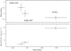 |
Fig. 6. Orbital phase dependence of the power law spectral parameters of lowest intensity states observed during the two XMM–Newton observations (performed in 2007 and 2020) and the Suzaku one. The power-law photon index and unabsorbed flux (in units of 10−13 erg cm−2 s−1) are reported in the upper and lower panels, respectively (see Sect. 5 for details). |
6. Discussion
We investigated the X-ray properties shown by the SFXT IGR J08408-4503 during an observation performed by XMM–Newton in June 2020, which caught the source just after the apastron, in its lowest X-ray emission state, to date. The source X-ray light curve shows a faint, short flare (which is usual in SFXTs, even at low-luminosity states, e.g., Sidoli et al. 2019), with emission becoming harder when brighter. This behavior led us to investigate X-ray spectra extracted from three different intervals of source count rate separately. The lowest state spectrum is well deconvolved by a three-component model, with a two-temperature hot plasma model and a power law. The temperatures of the thermal components (kT = 0.24 keV and kT = 0.76 keV) are consistent with the usual X-ray emission observed from O-type supergiants, highlighting the fact that the donor is a quite normal star. We ascribe the faint power-law component to residual accretion onto the compact object.
The source has previously been caught in a low X-ray state (1032 − 1033 erg s−1), with a low absorption and evidence of a soft component (Leyder et al. 2007; Bozzo et al. 2010; Sidoli et al. 2010). Although these authors already suggested that the soft component could be due to shocks in the supergiant wind, this is the first time that its presence has been clearly established in the source spectrum, thanks to the very low accretion onto the compact object and the high-throughput XMM–Newton observation. Therefore, the scenario emerging from the spectroscopy of the lowest luminosity state reveals that the unabsorbed flux contributed by the power-law component alone (e.g., accretion onto the compact object) is  erg cm−2 s−1 (0.5–10 keV), implying a luminosity of only (4.8 ± 1.4)×1031 erg s−1 due to accretion. In the following Sects. 6.1 and 6.2, we outline a physical scenario to explain this very low level of accretion.
Lastly, this picture is confirmed by the comparison with previous low states observed in IGR J08408-4503 with XMM–Newton and Suzaku (Sect. 5): our best fit to the X-ray emission from the supergiant donor is able to account for the softest region of the spectrum in those observations as well, while a brighter and harder power-law component (due to accretion) emerges, toward periastron passage.
6.1. Physical picture of the low-luminosity state of SFXTs
We assume that accretion in SFXTs proceeds quasi-spherically onto a slowly rotating magnetized NS from the optical companion’s stellar wind (Shakura et al. 2014; see e.g., Kretschmar et al. 2019 for a recent review). The accreting plasma enters the magnetosphere via the Rayleigh-Taylor instability (RTI). A steady mass accretion rate is possible if plasma arriving at the magnetosphere cools down below a certain critical temperature (Elsner & Lamb 1977). The Compton cooling by X-rays generated near the NS surface is effective above the critical X-ray luminosity L† ≃ 4 × 1036 erg s−1. At lower luminosities, a hot, convective atmosphere grows above the NS magnetosphere filling the space up to roughly the Bondi capture radius RB.
Through this hot (likely convective) shell a quasi-steady subsonic, settling accretion regime is established: the accretion is controlled by the plasma cooling mechanism and occurs at a rate Ṁ ≈ f(u) ṀB, where  is the Bondi (supersonic) capture rate (the subscript m means that the plasma density ρ and free-fall velocity are evaluated near the magnetospheric radius Rm). The factor f(u)≈(tff/tcool)1/3 < 1 is determined by the ratio of the free-fall time tff to the plasma cooling time tcool. At low X-ray luminosities, LX ≪ L†, the quasi-steady plasma entry rate is mediated by radiative cooling. In this case (Shakura et al. 2013),
 (1)
(1)
Here, L36 ≡ Lx/(1036 erg s−1) = 0.1 × 10¹⁶[g s−1] Ṁx,16c2 is the accretion X-ray luminosity, the NS magnetic moment is in units of 1030 G cm3, and the numerical coefficient is calculated for a 1.5 M⊙ NS. It is convenient to express this factor through the gravitational capture Bondi rate ṀB, which is related to the accretion rate for the radiative cooling as  (Yungelson et al. 2019):
 (2)
(2)
We stress that Eq. (1) is appropriate when the accretion X-ray luminosity is known, while Eq. (2) uses the Bondi mass capture rate that is not directly measurable but can be estimated from stellar wind and the binary system’s parameters.
In this model, sporadic X-ray outbursts in SFXTs can be due to magnetospheric instability triggered, for example, by magnetic reconnection with external stellar wind magnetic field carried by plasma blobs close to the magnetospheric boundary (Shakura et al. 2014 and below).
The condition for the RTI to be effective can be formulated as the requirement for plasma to cool down below a critical temperature depending on the magnetosphere’s curvature (Elsner & Lamb 1977). In a convective shell around the NS magnetosphere, the convection lifts up the hot gas from the magnetospheric boundary. Therefore, for an effective RTI to occur, the plasma cooling time near the magnetosphere should be shorter than the convective overturn time, tcool < tconv. The radiative cooling time is (Shakura et al. 2013)
![Mathematical equation: $$ \begin{aligned} t_\mathrm{rad} \approx 300 \,[\mathrm {s}] \mu _{30}^{2/3}\dot{M}_\mathrm{x,16} ^{-1}\approx 6000 \,[\mathrm {s}] \mu _{30}^{4/7}\dot{M}_\mathrm{B,16} ^{-9/7} . \end{aligned} $$](/articles/aa/full_html/2021/10/aa41378-21/aa41378-21-eq66.gif) (3)
(3)
The longest convection overturn time is commensurable with the free-fall time from the Bondi radius,  :
:
![Mathematical equation: $$ \begin{aligned} t_\mathrm{conv} =\zeta _c t_\mathrm{ff} (R_\mathrm{B} )\simeq 400\,[\mathrm {s}] \zeta _c { v}_8^{-3}\,, \end{aligned} $$](/articles/aa/full_html/2021/10/aa41378-21/aa41378-21-eq68.gif) (4)
(4)
where the dimensionless factor ζc ≳ 1, and the stellar wind velocity relative to the NS vw = 108cm s−1v8. Therefore, for radiative plasma cooling, we expect the RTI to operate when
 (5)
(5)
For an NS moving around an optical star with a mass-loss rate of ṀO = 10−6(M⊙ yr−1) ṀO,−6, the Bondi capture rate is ṀB,16 ≈104/(2π)ṀO,−6(RB/r)2 (here, r is the distance from the optical star to the NS). Thus, the condition (5) can be recast to the form
 (6)
(6)
For example, it is easy to check that the condition (6) can be met for systems like Vela X-1 with v8 ∼ 0.7, μ30 = 1.2 and r ≈ 50 R⊙ for ζc∼ a few1.
What happens if the accretion rate onto an NS in a binary system drops below the critical value (5), and the magnetosphere turns out to be Rayleigh-Taylor stable? This could be the case for an NS moving in an elliptic orbit near apastron. Then, the quasi-static plasma entry can be sustained by (i) the diffusion through the magnetosphere, (ii) the magnetospheric cusp instability, or (iii) magnetic reconnection with magnetic field carried out by accreting stellar wind blobs (Elsner & Lamb 1984).
Of these possible physical mechanisms, the most effective is the entry via turbulent plasma diffusion in the Bohm regime. An extreme upper bound on the plasma entry rate can be obtained from Eq. (59) of Elsner & Lamb (1984) applied to the settling accretion regime. In this case, we should take into account that in the settling accretion regime the magnetospheric radius differs from the reference Alfvén value,  (see Shakura et al. 2012):
![Mathematical equation: $$ \begin{aligned} R_\mathrm{m} \approx \left[\frac{4\gamma }{(\gamma -1)}K_2 f(u)\right]^{2/7}R_{\rm A}\,. \end{aligned} $$](/articles/aa/full_html/2021/10/aa41378-21/aa41378-21-eq72.gif) (7)
(7)
For the accretion of a monoatomic gas with adiabatic index γ = 5/3, the factor in the brackets in the above equation takes into account the magnetospheric current’s boundary screening (Arons & Lea 1976) and is equal to 76.2. For the radiative plasma cooling, the magnetospheric radius reads (Shakura et al. 2013)
![Mathematical equation: $$ \begin{aligned} R_\mathrm{m} \approx 10^9 [\mathrm{cm} ]\mu _{30}^{16/27} L_\mathrm{36} ^{-2/9}\simeq 2\times 10^9[\mathrm{cm} ]\mu _{30}^{4/7}\dot{M}_\mathrm{B,16} ^{-2/7}\,. \end{aligned} $$](/articles/aa/full_html/2021/10/aa41378-21/aa41378-21-eq73.gif) (8)
(8)
In the second equation, we changed the X-ray luminosity L36 by ṀB,16 in a way as in Eqs. (1) and (2). As the Bondi mass-accretion rate enters Eq. (32) of Elsner & Lamb (1984), determining the Bohm diffusion through the magnetosphere via the Alfven radius RA, we should change Ṁ → ṀB/(76f(u)rad) in Eq. (59) of Elsner & Lamb (1984). Then, using formula (2) for f(u)rad through ṀB, we arrive at a maximum suppression factor of the free-fall Bondi accretion rate due to the Bohm-diffusion in the radiation-cooling settling regime:
 (9)
(9)
We note a very weak dependence on the (unknown) NS magnetic field. For practical use, we can recast formula (9) to the following form:
![Mathematical equation: $$ \begin{aligned} \dot{M}_\mathrm{dif} \simeq 3.3 \times 10^{11} [\mathrm {g}\,\mathrm {s}^{-1} ] \dot{M}_\mathrm{B,16} ^{83/98}\mu _{30}^{-5/98}\,. \end{aligned} $$](/articles/aa/full_html/2021/10/aa41378-21/aa41378-21-eq75.gif) (10)
(10)
Thus, in SFXTs, at a given Bondi gravitational capture rate ṀB determined by the orbital parameters and stellar wind properties of the optical star, there should be a minimum possible accretion X-ray luminosity in the low states of SFXTs:
![Mathematical equation: $$ \begin{aligned} L_\mathrm{X,min} \sim 3.3\times 10^{31}[\mathrm {erg}\,\mathrm {s}^{-1} ]\dot{M}_\mathrm{B,16} ^{83/98}\mu _{30}^{-5/98}\,. \end{aligned} $$](/articles/aa/full_html/2021/10/aa41378-21/aa41378-21-eq76.gif) (11)
(11)
6.2. Application to IGR J08408-4503
6.2.1. Minimum X-ray luminosity.
Equations (9) and (11) suggest that an almost universal lower limit to mass-accretion rates in SFXTs should exist with the radiation-cooling settling accretion. Its value is proportional to the Bondi mass-accretion rate,  . By knowing (or assuming) the stellar wind mass-loss rate, the Bondi capture rate can be estimated from the binary system parameters. For example, we can use the recent semi-analytical analysis of Bozzo et al. (2021), which shows that for IGR J08408-4503, the expected Bondi mass-accretion rate should be around 3 × 10¹⁵ − 1016 g s−1 (see their Fig. 7, left panel). With these Bondi capture rates, the condition (5) can be violated at the orbital phases of the XMM–Newton observations, which turn out to be RTI-stable. Substituting ṀB,16 ∼ 1 into Eq. (11), we obtain LX, min ≈ 3.3 × 1031 erg s−1 for IGR J08408-4503, which is slightly below the observed lowest X-ray luminosity. The factor of two uncertainty in the stellar wind parameters of LM Vel are possible (Hainich et al. 2020). For example, a slight increase in the wind mass-loss rate from the optical star, or an insignificant decrease in the stellar wind velocity could easily bring the expected residual X-ray luminosity of IGR J08408-4503 into agreement with the observed 5 × 1031 erg s−1.
We note that Bozzo et al. (2021) introduce an accretion suppression of factor χ = 7 × 10⁻⁵ by hand to match the observed low luminosities of IGR J08408-4503 at periastron (see Fig 7, right panel in Bozzo et al. 2021). In our formulation, the low X-ray luminosity between SFXT flares is due to plasma entry into the magnetosphere at the radiation-driven settling accretion stage (see Sidoli et al. 2019 for more details). Therefore, this factor naturally arises from our physical model (see Eq. (9)). No additional ‘suppression’ of accretion is needed. Thus, our estimates show that the expected maximum diffusion mass-accretion rate in the low states of SFXTs can be as low as a few 1031 erg s−1, in agreement with what is observed.
6.2.2. The lack of strong flaring activity.
One may wonder why we do not see bright X-ray flares at apastron phases of IGR J08408-4503. We note that in the first place the orbital phases of IGR J08408-4503 around apastron are RTI-stable (the condition (5) is violated for the expected Bondi capture rates). In our formulation, the lack of bright outbursts means that the possible magnetic reconnection is less effective at orbital phases ∼0.1 − 0.6 around apastron. To see this, we consider the magnetic reconnection of a plasma blob2 with size λRm (λ ≪ 1), density ρ′∼ρm and magnetic field B′=αBm with the magnetospheric field Bm. The reconnection time is tr = λRm/ur; the reconnection rate is ur = ϵruA, where  is the Alfvenic velocity in the weaker-field blob; and ϵr ∼ 0.01 − 0.1 is the reconnection efficiency. By definition, the magnetospheric radius at the settling accretion stage is
  , where
  is the thermal sound velocity near the magnetosphere (Shakura et al. 2012). Noticing that the free-fall velocity at the magnetosphere is
  , we find:
  .
.
For an effective reconnection to occur, the reconnection time should be shorter than the time the blob spends near the magnetospheric boundary, the convection overturn time, tr < tff(RB) = ζctff(RB):
 (12)
(12)
It is clear that this ratio strongly depends on the wind velocity. The numerical coefficient here is determined by the scale λ and amplitude α of the magnetic cell. During turbulent plasma infall,  , α ≲ 1, and the turbulent cell size can be λt ≲ 1. In the case of IGR J08408-4503, the relative wind velocity increases from ∼500 km s−1 at periastron to ∼1400 km s−1 at apastron (Hainich et al. 2020), changing the ratio tr/tff by a factor of ∼30 over the orbit. Thus, the violation of the inequality (12) can explain the transition from the flaring state near periastron to quiescent behavior close to apastron.
6.2.3. Magnetized stellar wind effects in SFXTs.
The effect of a magnetized stellar wind in HMXBs can be twofold. First, the magnetic reconnection of blobs with embedded magnetic field B′ comparable to the field at the magnetospheric boundary Bm can dramatically disturb (even open) the NS magnetosphere leading to bright SFXT outbursts (Shakura et al. 2014). Second, the magnetic reconnection of small-size blobs at the base of the shell around the magnetosphere, which does not strongly disturb the magnetospheric boundary, would additionally heat the plasma. This heating could further hinder the RTI development, hamper the plasma entry, and strengthen the convection in the shell (Shakura et al. 2012). It is tempting to suggest that the additional reconnection-induced plasma heating in magnetized plasma blobs occurs even at the periastron of IGR J08408-4503 (where the RTI condition (5) is evidently met). This could be responsible for an increased SFXT activity at the periastron but not for the full turning-on of the RTI-mediated accretion on the NS in this source.
The moderate flare of IGR J08408-4503 detected during our observations (see Fig. 1) can be the manifestation of a sporadic magnetic reconnection in the RTI-stable hot shell. Indeed, the mass of the settling shell is ΔMrad ≃ 3.7 × 10¹⁵(vw/1000 km s−1)−3 g (Shakura et al. 2014). If the magnetospheric instability is sporadically caused by the magnetic reconnection with a large magnetized stellar wind clump with λ ∼ 1, the characteristic time of an outburst will be on the order of the free-fall time from the Bondi radius tff ∼ 103 s (see Fig. 2). Therefore, the X-ray luminosity of the outburst should be about 1033 erg s−1, which is close to the observed value.
Among O-type stars, the stars with Of?p spectral types are recognized as strongly magnetic (Walborn et al. 2010; Grunhut et al. 2017). In these stars, as well as as in some magnetic O-dwarfs, magnetic field strongly influences the dynamics of stellar winds. In X-rays, the magnetic O-type dwarfs are harder and brighter compared to their non-magnetic counterparts (e.g., Schulz et al. 2000; Shenar et al. 2017). Direct searches for a regular magnetic field in LM Vel have failed so far (Hubrig et al. 2018). However, weak, 50–100 G magnetic fields with a complex topology have been detected in the spectroscopically similar O9.7Ib supergiant ζ Ori (Bouret et al. 2008). The X-ray properties of ζ Ori are usual for its spectral type (Waldron & Cassinelli 2007) with no signs of a power-law continuum detected in the X-ray spectrum of this well-studied star.
7. Conclusions
The XMM–Newton observation of the SFXT IGR J08408-4503 performed in 2020 caught the source in a very low level of X-ray activity, with a flux of 3.2 × 10⁻¹³ erg cm−2 s−1 (0.5–10 keV, corrected for the interstellar absorption). The X-ray spectrum is well described by a three-component model: two thermal plasma models (showing temperatures of kT1 = 0.24 keV and kT2 = 0.76 keV), together with a power law (Γ = 2.55) that dominates emission above ∼2 keV and contributes about 25% of the X-ray flux in the 0.5–10 keV energy range.
We argue that the power-law X-ray component of IGR J08408-4503 observed during XMM–Newton observations at the orbital phases ϕ ∼ 0.65 at a level of LX ≃ 5 × 1031 erg s−1 can be explained by the diffusion plasma entry rate into the NS magnetosphere at the radiation-dominated settling accretion stage. The mild flaring activity at these orbital phases of IGR J08408-4503 can be due to reconnection in magnetized stellar wind blobs arriving at the magnetosphere, as proposed by us earlier (Shakura et al. 2014; Sidoli et al. 2019). Notably, the diffusion accretion rate at low states of SFXTs (Eq. (9)) is almost independent of the NS magnetic field and almost linearly depends on the Bondi accretion rate from the stellar wind of the optical star. The minimum possible accretion luminosity in this case would be LX, min ∼ 3 × 1031 erg s−1. The timing X-ray properties of the diffusion entry should be different from those supposedly observed in SFXTs where the RTI operates (Sidoli et al. 2019). It would be interesting to further investigate the low (unflared) state of other SFXTs to check our models.
The observations of IGR J08408-4503 at its lowest state allowed us to detect the intrinsic X-ray emission from the O-type supergiant donor star. The properties of the donor star’s X-ray emission are very similar to those of other O-supergiants: log LX ≈ 32.7 [erg s−1] and the X-ray spectrum well described by a thermal, collisionally ionized plasma model with TX≈ 3–10 MK. The discovery of average X-ray properties further highlights the fact that the donor star is not a peculiar object but has usual (for its spectral type) stellar and wind properties.
In Vela X-1, however, the Compton plasma cooling should be more effective most of the time (see Shakura et al. 2012, 2013).
The magnetized blobs near the NS magnetosphere are different from the stellar-wind “clumps”; they can appear in the convective settling shell even in the case of gravitational capture of an almost homogeneous stellar wind.
Acknowledgments
This work is based on data from observations with XMM–Newton, an ESA science mission with instruments and contributions directly funded by ESA Member States and NASA. We thank our anonymous referee for the very constructive report and useful comments that helped to improve the clarity of our writing. LMO acknowledges partial support by the Russian Government Program of Competitive Growth of Kazan Federal University. The work of KP was partially supported by RFBR grant 19-02-00790.
References
- Arnaud, K. A. 1996, in Astronomical Data Analysis Software and Systems V, eds. G. H. Jacoby, & J. Barnes, ASP Conf. Ser., 101, 17 [NASA ADS] [Google Scholar]
- Arons, J., & Lea, S. M. 1976, ApJ, 207, 914 [Google Scholar]
- Bailer-Jones, C. A. L., Rybizki, J., Fouesneau, M., Demleitner, M., & Andrae, R. 2021, AJ, 161, 147 [Google Scholar]
- Barba, R., Gamen, R., & Morrell, N. 2006, ATel, 819, 1 [NASA ADS] [Google Scholar]
- Berghoefer, T. W., Schmitt, J. H. M. M., Danner, R., & Cassinelli, J. P. 1997, A&A, 322, 167 [Google Scholar]
- Bohlin, R. C., Savage, B. D., & Drake, J. F. 1978, ApJ, 224, 132 [Google Scholar]
- Bouret, J. C., Donati, J. F., Martins, F., et al. 2008, MNRAS, 389, 75 [NASA ADS] [CrossRef] [Google Scholar]
- Bozzo, E., Falanga, M., & Stella, L. 2008, ApJ, 683, 1031 [Google Scholar]
- Bozzo, E., Stella, L., Ferrigno, C., et al. 2010, A&A, 519, A6 [NASA ADS] [CrossRef] [EDP Sciences] [Google Scholar]
- Bozzo, E., Ducci, L., & Falanga, M. 2021, MNRAS, 501, 2403 [NASA ADS] [CrossRef] [Google Scholar]
- Cassinelli, J. P., Waldron, W. L., Sanders, W. T., et al. 1981, ApJ, 250, 677 [NASA ADS] [CrossRef] [Google Scholar]
- den Herder, J. W., Brinkman, A. C., Kahn, S. M., et al. 2001, A&A, 365, L7 [NASA ADS] [CrossRef] [EDP Sciences] [Google Scholar]
- Ducci, L., Romano, P., Ji, L., & Santangelo, A. 2019, A&A, 631, A135 [NASA ADS] [CrossRef] [EDP Sciences] [Google Scholar]
- Elsner, R. F., & Lamb, F. K. 1977, ApJ, 215, 897 [NASA ADS] [CrossRef] [Google Scholar]
- Elsner, R. F., & Lamb, F. K. 1984, ApJ, 278, 326 [NASA ADS] [CrossRef] [Google Scholar]
- Feldmeier, A., Puls, J., & Pauldrach, A. W. A. 1997, A&A, 322, 878 [NASA ADS] [Google Scholar]
- Foight, D. R., Güver, T., Özel, F., & Slane, P. O. 2016, ApJ, 826, 66 [Google Scholar]
- Gaia Collaboration (Brown, A. G. A., et al.) 2021, A&A, 649, A1 [NASA ADS] [CrossRef] [EDP Sciences] [Google Scholar]
- Gamen, R., Barbà, R. H., Walborn, N. R., et al. 2015, A&A, 583, L4 [NASA ADS] [CrossRef] [EDP Sciences] [Google Scholar]
- Giménez-García, A., Shenar, T., Torrejón, J. M., et al. 2016, A&A, 591, A26 [EDP Sciences] [Google Scholar]
- Götz, D., Schanne, S., Rodriguez, J., et al. 2006, ATel, 813, 1 [NASA ADS] [Google Scholar]
- Götz, D., Falanga, M., Senziani, F., et al. 2007, ApJ, 655, L101 [CrossRef] [Google Scholar]
- Grebenev, S. A., & Sunyaev, R. A. 2007, Astron. Lett., 33, 149 [NASA ADS] [CrossRef] [Google Scholar]
- Grunhut, J. H., Wade, G. A., Neiner, C., et al. 2017, MNRAS, 465, 2432 [NASA ADS] [CrossRef] [Google Scholar]
- Gudennavar, S. B., Bubbly, S. G., Preethi, K., & Murthy, J. 2012, ApJS, 199, 8 [NASA ADS] [CrossRef] [Google Scholar]
- Hainich, R., Oskinova, L. M., Torrejón, J. M., et al. 2020, A&A, 634, A49 [NASA ADS] [CrossRef] [EDP Sciences] [Google Scholar]
- Harnden, Jr., F. R., Branduardi, G., Elvis, M., et al. 1979, ApJ, 234, L51 [NASA ADS] [CrossRef] [Google Scholar]
- Hubrig, S., Sidoli, L., Postnov, K., et al. 2018, MNRAS, 474, L27 [NASA ADS] [CrossRef] [Google Scholar]
- Huenemoerder, D. P., Ignace, R., Miller, N. A., et al. 2020, ApJ, 893, 52 [NASA ADS] [CrossRef] [Google Scholar]
- in’t Zand, J. J. M. 2005, A&A, 441, L1 [CrossRef] [EDP Sciences] [Google Scholar]
- Jansen, F., Lumb, D., Altieri, B., et al. 2001, A&A, 365, L1 [NASA ADS] [CrossRef] [EDP Sciences] [Google Scholar]
- Kennea, J. A., & Campana, S. 2006, ATel, 818, 1 [NASA ADS] [Google Scholar]
- Kretschmar, P., Fürst, F., Sidoli, L., et al. 2019, New Astron. Rev., 86 [Google Scholar]
- Lamers, H. J. G. L. M., & Cassinelli, J. P. 1999, Introduction to Stellar Winds [Google Scholar]
- Leyder, J. C., Walter, R., Lazos, M., Masetti, N., & Produit, N. 2007, A&A, 465, L35 [NASA ADS] [CrossRef] [EDP Sciences] [Google Scholar]
- Liszt, H. 2014, ApJ, 780, 10 [Google Scholar]
- Martínez-Núñez, S., Kretschmar, P., Bozzo, E., et al. 2017, Space Sci. Rev., 212, 59 [Google Scholar]
- Masetti, N., Bassani, L., Bazzano, A., et al. 2006, ATel, 815, 1 [NASA ADS] [Google Scholar]
- Massa, D., Oskinova, L., Prinja, R., & Ignace, R. 2019, ApJ, 873, 81 [NASA ADS] [CrossRef] [Google Scholar]
- Mereghetti, S., Sidoli, L., Paizis, A., & Götz, D. 2006, ATel, 814, 1 [NASA ADS] [Google Scholar]
- Nazé, Y. 2009, A&A, 506, 1055 [NASA ADS] [CrossRef] [EDP Sciences] [Google Scholar]
- Nebot Gómez-Morán, A., & Oskinova, L. M. 2018, A&A, 620, A89 [NASA ADS] [CrossRef] [EDP Sciences] [Google Scholar]
- Negueruela, I., Smith, D. M., Reig, P., Chaty, S., & Torrejón, J. M. 2006, in Proc. of the “The X-ray Universe 2005”, 26–30 September 2005, El Escorial, Madrid, Spain, ed. A. Wilson (Noordwijk: ESA Pub. Division), 1, ESA SP, 604 [Google Scholar]
- Oskinova, L. M. 2016, Adv. Space Res., 58, 739 [NASA ADS] [CrossRef] [Google Scholar]
- Predehl, P., & Schmitt, J. H. M. M. 1995, A&A, 293, 889 [NASA ADS] [Google Scholar]
- Puls, J., Vink, J. S., & Najarro, F. 2008, A&ARv, 16, 209 [NASA ADS] [CrossRef] [Google Scholar]
- Rampy, R. A., Smith, D. M., & Negueruela, I. 2009, ApJ, 707, 243 [NASA ADS] [CrossRef] [Google Scholar]
- Rauw, G., & Nazé, Y. 2016, Adv. Space Res., 58, 761 [Google Scholar]
- Rauw, G., Hervé, A., Nazé, Y., et al. 2015, A&A, 580, A59 [NASA ADS] [CrossRef] [EDP Sciences] [Google Scholar]
- Romano, P. 2015, J. High Energy Astrophys., 7, 126 [Google Scholar]
- Romano, P., Sidoli, L., Mangano, V., Mereghetti, S., & Cusumano, G. 2007, A&A, 469, L5 [NASA ADS] [CrossRef] [EDP Sciences] [Google Scholar]
- Romano, P., Sidoli, L., Cusumano, G., et al. 2009, MNRAS, 392, 45 [NASA ADS] [CrossRef] [Google Scholar]
- Sander, A. A. C. 2019, IAU Symp., 346, 17 [NASA ADS] [Google Scholar]
- Schulz, N. S., Canizares, C. R., Huenemoerder, D., & Lee, J. C. 2000, ApJ, 545, L135 [Google Scholar]
- Sguera, V., Barlow, E. J., Bird, A. J., et al. 2005, A&A, 444, 221 [NASA ADS] [CrossRef] [EDP Sciences] [Google Scholar]
- Sguera, V., Bazzano, A., Bird, A. J., et al. 2006, ApJ, 646, 452 [NASA ADS] [CrossRef] [Google Scholar]
- Shakura, N., Postnov, K., Kochetkova, A., & Hjalmarsdotter, L. 2012, MNRAS, 420, 216 [Google Scholar]
- Shakura, N., Postnov, K., & Hjalmarsdotter, L. 2013, MNRAS, 428, 670 [NASA ADS] [CrossRef] [Google Scholar]
- Shakura, N., Postnov, K., Sidoli, L., & Paizis, A. 2014, MNRAS, 442, 2325 [Google Scholar]
- Shenar, T., Oskinova, L. M., Järvinen, S. P., et al. 2017, A&A, 606, A91 [NASA ADS] [CrossRef] [EDP Sciences] [Google Scholar]
- Sidoli, L. 2017, Proceedings of the XII Multifrequency Behaviour of High Energy Cosmic Sources Workshop. 12–17 June, 2017 Palermo, Italy (MULTIF2017), Online at https://pos.sissa.it/cgi-bin/reader/conf.cgi?confid=306 [Google Scholar]
- Sidoli, L., & Paizis, A. 2018, MNRAS, 481, 2779 [NASA ADS] [CrossRef] [Google Scholar]
- Sidoli, L., Romano, P., Mangano, V., et al. 2008, ApJ, 687, 1230 [NASA ADS] [CrossRef] [Google Scholar]
- Sidoli, L., Romano, P., Ducci, L., et al. 2009, MNRAS, 397, 1528 [NASA ADS] [CrossRef] [Google Scholar]
- Sidoli, L., Esposito, P., & Ducci, L. 2010, MNRAS, 409, 611 [CrossRef] [Google Scholar]
- Sidoli, L., Paizis, A., & Postnov, K. 2016, MNRAS, 457, 3693 [NASA ADS] [CrossRef] [Google Scholar]
- Sidoli, L., Postnov, K. A., Belfiore, A., et al. 2019, MNRAS, 487, 420 [Google Scholar]
- Sota, A., Maíz Apellániz, J., Morrell, N. I., et al. 2014, ApJS, 211, 10 [Google Scholar]
- Steinberg, E., & Metzger, B. D. 2018, MNRAS, 479, 687 [NASA ADS] [Google Scholar]
- Strüder, L., Briel, U., Dennerl, K., et al. 2001, A&A, 365, L18 [Google Scholar]
- Turner, M. J. L., Abbey, A., Arnaud, M., et al. 2001, A&A, 365, L27 [CrossRef] [EDP Sciences] [Google Scholar]
- Verner, D. A., Ferland, G. J., Korista, K. T., & Yakovlev, D. G. 1996, ApJ, 465, 487 [Google Scholar]
- Vink, J. S., & Sander, A. A. C. 2021, MNRAS, 504, 2051 [NASA ADS] [CrossRef] [Google Scholar]
- Vuong, M. H., Montmerle, T., Grosso, N., et al. 2003, A&A, 408, 581 [NASA ADS] [CrossRef] [EDP Sciences] [Google Scholar]
- Waldron, W. L., & Cassinelli, J. P. 2007, ApJ, 668, 456 [NASA ADS] [CrossRef] [Google Scholar]
- Walborn, N. R., Sota, A., Maíz Apellániz, J., et al. 2010, ApJ, 711, L143 [NASA ADS] [CrossRef] [Google Scholar]
- Walter, R., Lutovinov, A. A., Bozzo, E., & Tsygankov, S. S. 2015, A&A Rv., 23, 2 [NASA ADS] [Google Scholar]
- Wilms, J., Allen, A., & McCray, R. 2000, ApJ, 542, 914 [Google Scholar]
- Yungelson, L. R., Kuranov, A. G., & Postnov, K. A. 2019, MNRAS, 485, 851 [NASA ADS] [CrossRef] [Google Scholar]
- Zhu, H., Tian, W., Li, A., & Zhang, M. 2017, MNRAS, 471, 3494 [NASA ADS] [CrossRef] [Google Scholar]
Appendix A: Lowest emission state: Additional models
For the sake of completeness, we report in Table A.1 the spectral parameters obtained when fitting the spectrum of the lowest state with the six models discussed in Sect. 4.1. All models resulted in equally good deconvolutions of the spectrum. However, the expected X-ray emission from the supergiant donor itself favors the two APEC models (Model 3, in Table A.1). Nevertheless, some issues remain when adopting Model 3, as discussed in Sect. 4.1. In conclusion, for better clarity, our preferred final deconvolution of the spectrum is reported in Table 2 (Model 2).
We note that in Table A.1 the uncertainty on the emission measure of the thermal emission model APEC in XSPEC (EMAPEC) was derived only from the error on the normalization of the thermal model (i.e., no uncertainty on the distance was considered). We always adopt solar abundances in the APEC model.
Spectroscopy of the lowest luminosity state (EPIC pn, MOS1, and MOS2) with statistically acceptable models (see Sect. A and Sect. 4.1 for details and issues).
All Tables
Spectroscopy of the lowest luminosity state (EPIC pn, MOS1, and MOS2), fixing the absorption to the optical value toward LM Vel (NH = 3.9 × 1021 cm−2).
Spectroscopy of the lowest luminosity state (EPIC pn, MOS1, and MOS2) with statistically acceptable models (see Sect. A and Sect. 4.1 for details and issues).
All Figures
|
Fig. 1. Source light curve (EPIC pn, not background subtracted, bin time = 256 s) in two energy ranges (Soft = 0.3–2 keV, Hard = 2–12 keV), together with their hardness ratio. The first ∼6000 s of the observation have been excluded because of high background level. |
| In the text | |
|
Fig. 2. Source light curve (EPIC pn, 1–10 keV, not background subtracted, bin time = 100 s), where the horizontal lines mark the three count rate intervals adopted for the intensity selected spectroscopy: interval 1 (lowest state), 2 (intermediate state), and 3 (the faint flare). |
| In the text | |
|
Fig. 3. EPIC spectra extracted from the lowest state, fit by a single absorbed power-law model. Upper panel: count spectra, lower panel: residuals with respect to the model in terms of standard deviation. The meaning of the symbols is the following: crosses, empty circles, and solid squares mark the EPIC pn, MOS1, and MOS2 spectra, respectively. |
| In the text | |
|
Fig. 4. Best fit of the IGR J08408-4503 spectra extracted during the lowest luminosity state (lower panel; Model 2 in Table 2), the intermediate state (middle panel; Model C in Table 3), and the faint flare (upper panel; Model B in Table 4). The counts spectra are plotted together with the residuals in units of standard deviation. The meaning of the symbols are the same as in Fig. 3. |
| In the text | |
|
Fig. 5. Comparison of Suzaku (on the left) and XMM–Newton observations performed in 2007 (on the right) with the best fit of the lowest luminosity state observed in 2020 with XMM–Newton. Residuals are reported in the lower panels in units of standard deviations. The meaning of the symbols in the right panel is the following: crosses, empty circles, and solid squares mark the EPIC pn, MOS1, and MOS2 spectra, respectively. Clearly, past observations caught IGR J08408-4503 in harder states. |
| In the text | |
|
Fig. 6. Orbital phase dependence of the power law spectral parameters of lowest intensity states observed during the two XMM–Newton observations (performed in 2007 and 2020) and the Suzaku one. The power-law photon index and unabsorbed flux (in units of 10−13 erg cm−2 s−1) are reported in the upper and lower panels, respectively (see Sect. 5 for details). |
| In the text | |
Current usage metrics show cumulative count of Article Views (full-text article views including HTML views, PDF and ePub downloads, according to the available data) and Abstracts Views on Vision4Press platform.
Data correspond to usage on the plateform after 2015. The current usage metrics is available 48-96 hours after online publication and is updated daily on week days.
Initial download of the metrics may take a while.