| Issue |
A&A
Volume 654, October 2021
|
|
|---|---|---|
| Article Number | A142 | |
| Number of page(s) | 18 | |
| Section | Extragalactic astronomy | |
| DOI | https://doi.org/10.1051/0004-6361/202140396 | |
| Published online | 25 October 2021 | |
MUSE observations of the blue compact dwarf galaxy Haro 14
Data analysis and first results on morphology and stellar populations⋆
1
Institut für Astrophysik, Georg-August-Universität, Friedrich-Hund-Platz 1, 37077 Göttingen, Germany
e-mail: This email address is being protected from spambots. You need JavaScript enabled to view it.
2
Hamburger Sternwarte, Gojenbergsweg 112, 21029 Hamburg, Germany
3
Leibniz-Institut für Astrophysik (AIP), An der Sternwarte 16, 14482 Potsdam, Germany
4
Max Planck Institute for Solar System Research, Justus-von-Liebig-Weg 3, 37077 Göttingen, Germany
Received:
21
January
2021
Accepted:
31
May
2021
Abstract
Investigations of blue compact galaxies (BCGs) are essential to advancing our understanding of galaxy formation and evolution. BCGs are low-luminosity, low-metallicity, gas-rich objects that form stars at extremely high rates, meaning they are good analogs to the high-redshift star-forming galaxy population. Being low-mass starburst systems, they also constitute excellent laboratories in which to investigate the star formation process and the interplay between massive stars and their surroundings. This work presents results from integral field spectroscopic observations of the BCG Haro 14 taken with the Multi Unit Spectroscopic Explorer (MUSE) at the Very Large Telescope in wide-field adaptive optics mode. The large MUSE field of view (1′×1′ = 3.8 × 3.8 kpc2 at the adopted distance of 13 Mpc) enables simultaneous observations of the central starburst and the low-surface-brightness host galaxy, which is a huge improvement with respect to previous integral field spectroscopy of BCGs. From these data we built galaxy maps in continuum and in the brightest emission lines. We also generated synthetic broad-band images in the VRI bands, from which we produced color index maps and surface brightness profiles. We detected numerous clumps spread throughout the galaxy, both in continuum and in emission lines, and produced a catalog with their position, size, and photometry. This analysis allowed us to study the morphology and stellar populations of Haro 14 in detail. The stellar distribution shows a pronounced asymmetry; the intensity peak in continuum is not centered with respect to the underlying stellar host but is displaced by about 500 pc southwest. At the position of the continuum peak we find a bright stellar cluster that with Mv = −12.18 appears as a strong super stellar cluster candidate. We also find a highly asymmetric, blue, but nonionizing stellar component that occupies almost the whole eastern part of the galaxy. We conclude that there are at least three different stellar populations in Haro 14: the current starburst of about 6 Myr; an intermediate-age component of between ten and several hundred million years; and a red and regular host of several gigayears. The pronounced lopsidedness in the continuum and also in the color maps, and the presence of numerous stellar clusters, are consistent with a scenario of mergers or interactions acting in Haro 14.
Key words: galaxies: individual: Haro 14 / galaxies: dwarf / galaxies: stellar content / galaxies: ISM / galaxies: star formation
Based on observations made with ESO Telescopes at Paranal Observatory under programme ID 60.A-9186(A).
© ESO 2021
1. Introduction
Among the rich variety of galaxies, blue compact galaxies (BCGs), which are low-mass systems experiencing vigorous episodes of star formation (SF), constitute a relatively rare but extremely interesting galaxy type (Thuan & Martin 1981; Papaderos et al. 1996; Cairós et al. 2001a,b; Gil de Paz et al. 2003).
First, in the widely accepted scenario of a cold dark matter Universe, larger galaxies form hierarchically from the assembly of smaller systems (Kauffmann et al. 1993; Springel et al. 2006; Loeb & Furlanetto 2013). Therefore, dwarf objects are essential to our understanding of galaxy formation and evolution. Within dwarfs, BCGs are particularly relevant because they have low chemical abundances (Izotov & Thuan 1999; Kunth & Östlin 2000), high amounts of neutral gas (Thuan & Martin 1981; Gordon & Gottesman 1981; Salzer et al. 2002), high specific star formation rates (SFR, Hunter & Elmegreen 2004), and clumpy morphology (Cairós et al. 2001a; Gil de Paz et al. 2003), meaning that these systems constitute precious analogs to the star forming galaxies observed at higher redshifts.
Furthermore, BCGs are excellent targets with which to investigate the SF process as well as its trigger and propagation mechanism(s). The absence of spiral density waves or strong shear forces makes it possible to examine SF in a relatively simple environment (Hunter 1997) and, at the same time, provides evidence that an alternative mechanism must be in place. A lot of effort has been invested into finding out how the SF in BCGs is triggered and maintained, but no conclusive findings have been found so far (Brinks 1990; Taylor 1997; Hunter & Elmegreen 2004; Pustilnik et al. 2001; Brosch et al. 2004). However, recent observational results indicate that dwarf–dwarf mergers, interactions, or infalling gas may play a major role in the ignition of the burst in low-mass systems (López-Sánchez et al. 2012; Nidever et al. 2013; Stierwalt et al. 2015; Privon et al. 2017; Pearson et al. 2018; Zhang et al. 2020a,b; Cairós & González-Pérez 2020).
Finally, studies focusing on BCGs will help to understand the complex interplay between massive stellar feedback and the interstellar medium (ISM). The impact of stellar feedback is expected to be especially dramatic in a low-mass system: the lack of density waves and significant shear forces allows the expanding shells created by stellar winds and supernovae (SNe) to grow to larger sizes and live longer than in typical spirals (Tomisaka et al. 1981; McCray & Kafatos 1987; Walter 1999), and in a shallow potential well, these shells can easily break out of the galaxy disk, or even the halo (Heckman et al. 1990; De Young & Heckman 1994; Mac Low & Ferrara 1999; Veilleux et al. 2005). Starburst-driven winds are indeed often invoked to explain fundamental questions such as the luminosity–metallicity relation (Garnett 2002; Tremonti et al. 2004; Chisholm et al. 2018), the chemical enrichment of the intergalactic medium (Theuns et al. 2002; Springel & Hernquist 2003), or the formation of galaxies (Larson 1974; Dekel & Silk 1986; Kauffmann et al. 1994; Naab & Ostriker 2017). However, in spite of its unquestionable importance, massive stellar feedback remains a poorly understood phenomenon: its multi-phase nature and the complexity of the physics involved make it quite difficult to tackle, both analytically and numerically (McKee & Ostriker 2007; Somerville & Davé 2015; Naab & Ostriker 2017). High-quality data of nearby starburst galaxies can mitigate this problem by providing observational constraints on the feedback parameters (Martin 1997, 1998; Calzetti et al. 1999, 2004).
Motivated by the relevance of these topics, we initiated a project centered on the analysis of BCGs by means of integral field spectroscopy. The main goal of this project is to characterize the ongoing SF episode in a large sample of starbursting dwarf galaxies and to investigate its impact on the environment. Our first results have convincingly demonstrated that integral field spectrographs (IFS), providing simultaneously spectrophotometric and kinematic information for a large galaxy region, are the most advantageous approach to probing small, highly asymmetrical, and compact systems such as BCGs (Cairós et al. 2009a,b, 2010; Cairós et al. 2012, 2015; Cairós & González-Pérez 2017a,b, 2020). The advent of a new generation of wide-field IFSs in 8-m class telescopes considerably broadens the possibilities in this research field. In particular, the Multi Unit Spectroscopic Explorer (MUSE; Bacon et al. 2010), with its unique combination of high spatial and spectral resolution, large field of view (FoV), and extended wavelength range, has proven to be a powerful tool in BCG research (Bik et al. 2015, 2018; Cresci et al. 2017; Kehrig et al. 2018; Menacho et al. 2019, 2021).
This is the first in a series of publications presenting a spectrophotometric study of the BCG Haro 14 based on MUSE observations. Haro 14, with a luminosity of MB = −16.92 (Gil de Paz et al. 2003) and a metallicity of 12+log(O/H) = 8.2 ± 0.1 (Cairós & González-Pérez 2017a, hereafter CGP17a), is a good representative of the BCG class (see Table 1). In this first paper, we describe our observations and data processing, and discuss our results on the morphology, structure, and stellar populations of the galaxy.
Basic parameters for Haro 14.
2. Observations and data processing
2.1. The target galaxy: the BCG Haro 14
Haro 14 is a nearby dwarf galaxy designated as a BCG in the pioneering work by Thuan & Martin (1981). According to the morphological classification by Loose & Thuan (1986), it belongs to the most common BCG type, namely the iE BCGs–these comprise about 70% of the BCG population. Optical and near-infrared (NIR) imaging reveals that Haro 14, as the great majority of BCGs, is made of an irregular high-surface-brightness (HSB) region placed atop a smooth low-surface-brightness (LSB) underlying stellar component (Marlowe et al. 1997, 1999; Doublier et al. 1999, 2001; Gil de Paz et al. 2003; Gil de Paz & Madore 2005; Noeske et al. 2003; Hunter & Elmegreen 2006). One distinct peculiarity of our galaxy is its pronounced asymmetry: the HSB region is clearly off-center with respect to the outer isophotes–the intensity peak is displaced by about 500 pc southwest from the geometrical center of the galaxy (see Fig. 1 in this work and Noeske et al. 2003). Integrated spectrophotometry in the optical has been carried out by Hunter & Hoffman (1999) and Moustakas & Kennicutt (2006).
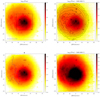 |
Fig. 1. Haro 14 as seen in broadband by MUSE. The FoV is ∼3.8 × 3.8 kpc2 and north is up and east to the left in all the maps presented in this paper. Top-left: image obtained by integrating over the whole observed spectral range. The blue bar corresponds to 1 kpc at the distance of Haro 14. The central square marks the FoV of our previous VIMOS observations. Top-right: “Pure continuum” image in the wavelength range 5400–5600 Å with contours over-plotted. The center of the outermost isophotes lies roughly around the position ΔRA ≃ +5″, ΔDec ≃ +2″. Lower-right: saturated pure continuum image to better visualize the dimmer external parts of the galaxy. Lower-left: synthetic image in the filter R. The color bar shows the calibrated surface brightness in units of mag arcsec−2, the ticks mark the position of two background emission galaxies (see Appendix) and the blue line roughly outlines the bluish regions of the galaxy at intermediate intensity levels (see Sect. 3.3). There are no foreground stars in the observed FoV. |
We included Haro 14 in our study of a sample of eight BCGs with the VIsible Multi-Object Spectrograph (VIMOS; Cairós et al. 2015, CGP17a). These works showed that the stellar and ionized gas distribution of the galaxy are significantly different: while in continuum the intensity peaks in two knots close to the galaxy center, the emission-line maps reveal an extended ongoing starburst resolved in numerous SF knots distributed over the whole mapped area (about 1.7 × 1.7 kpc2; see Fig. 1). The peaks in emission and continuum maps, which are considerably separated from each other, trace two spatially decoupled episodes of SF in the galaxy. Unfortunately, the VIMOS FoV does not completely cover the extended starburst and we find a plethora of incipient filaments and shells, a large concentration of dust, and evidence of shocked regions at the edge of the observed field, calling for integral field spectroscopy in a larger FoV.
2.2. Data acquisition
Haro 14 was observed with MUSE (Bacon et al. 2010) at the Very Large Telescope (VLT; ESO Paranal Observatory, Chile). MUSE is a panoramic IFS which, operating in its wide field mode (WFM), provides a FoV of 1′×1′ with a spatial sampling of 0 2.
2.
The observations were performed on September 2017 as part of the MUSE Adaptive Optics Facility (AOF) science verification run (Leibundgut et al. 2017). With the AOF, the MUSE WFM is supported by ground layer adaptive optics (GLAO) through four artificial laser guide stars and the adaptive optics system GALACSI (ground atmospheric optics for spectroscopic imaging).
The data were obtained in nominal mode (wavelength range 4750–9300 Å) with a spectral sampling of about 1.25 Å pix−1 in dispersion direction and an average resolving power of R ∼ 3000. There is a gap between ∼5800 and 5950 Å caused by the Na D blocking filter, because the AOF works with four sodium lasers and, otherwise, the detector would saturate. We took four 1370 s exposures of Haro 14, each rotated by 90° with respect to the previous one (a total of 5480 s on source). Because the target fills most of the MUSE FoV, we took separate sky fields of 120 s between the science exposures.
2.3. Data reduction
The data were processed using the standard MUSE pipeline (Weilbacher et al. 2016, 2020) working within the ESOREX environment with the default set of calibrations. The reduction follows the standard steps: bias and flat-field correction, tracing of the data on the CCD, and wavelength calibration. We applied geometric and astrometric calibrations from April 2017 and carried out a secondary spatial flat-field correction using a twilight cube. The flux calibration was carried out using exposures of the standard star EG 274, taken with the same instrumental mode the evening of the observations.
We determined the sky continuum from the offset sky field. In order to extract the sky lines we used the science exposures: we fit the lines in the outskirts of the field using a line spread function from June 2017 obtained for the same instrumental mode.
After correcting to barycentric velocities, we created cubes for all four science exposures. We used the white-light images to manually determine the centroid for the brightest continuum source in the field, and computed offsets relative to its Gaia DR1 position (Lindegren et al. 2016). We then combined all exposures using FWHM-based weighting. The final cube was sampled at the natural MUSE binning of  , resulting in a cube of 323 × 322 × 3681 voxels. The effective image quality is difficult to estimate because no bright foreground stars are visible in the field. From a fit of a Moffat profile to the brightest continuum source, we estimate that the spatial resolution is
  in the red and
  in the blue part of the spectrum.
2.4. Sky subtraction
The sky subtraction of the standard pipelines of integral field instruments often leaves significant systematic residuals. These residuals, which arise mainly from the imperfect estimation of the profiles of the telluric lines, can distort or even dominate the spectrum when the source is faint. An accurate modeling of the contribution of telluric lines is difficult because of the intrinsic spatio-temporal variability of the sky emission lines, imperfections of the spectrograph optics (e.g., distortions, flexures, and aberrations; Davies 2007; Hart 2019), the different characteristics of the optical fibers (in multi-fiber spectrographs), or the different optical paths from slice to slice (in spectrographs like MUSE with an image slicer). If the amplitude of the sky emission is underestimated (overestimated), emission (absorption) line residuals appear, whereas imperfect wavelength calibration produces P-Cygni-like profiles. Such miscorrections are particularly severe when the spectral lines are poorly sampled by the spectrograph, as is the case in MUSE (see, e.g., Fig. 3 in McLeod et al. 2015 or Fig. 2 in James et al. 2020).
Because we aim to accurately measure the flux in the LSB regions of Haro 14, we need to mitigate systematic residuals from telluric lines. The systematic errors left by the sky subtraction are correlated across extended wavelength ranges and the principal component analysis (PCA) has proven to be an excellent tool for the correction of residuals of telluric lines both for multi-fiber and image slicer IFS (Kurtz & Mink 2000; Wild & Hewett 2005; Sharp & Parkinson 2010; Hart 2019; Soto et al. 2016). We implemented a PCA-based method for the removal of telluric lines that is similar to the ZAP tool developed by Soto et al. (2016). Our routine consists of the following steps:
(1) Selection of the spaxels that contain only sky background. We search for sky-dominated spaxels, namely those without continuum or nebular line emission. These are defined as having a maximum Hα flux of 1.5 × 10⁻²⁰ erg s−1 cm−2 and a spectral flux density below 1.5 × 10⁻²⁰ erg s−1 cm−2 Å−1 in the continua adjacent to Hα and [O III]λ5007. To this end, we first run a test trial line fit to the data cube. We found 1322 spaxels with fluxes dominated by the sky emission.
(2) Subtraction of the continuum to keep only the lines. We remove the continuum of all spaxels in the image, including those dominated by the galaxy emission, applying a running-median filter to all spectra and then subtracting the original one from the median filtered spectra. The box-size of the median filter is 100 pixels (125 Å) which is small enough to estimate the shape of the continuum but large enough not to be affected by the spectral lines.
(3) Calculation of the spectral eigenvectors. The principal components, or eigenvectors, are calculated using the MATLAB routine PCA with the singular value decomposition algorithm. We carefully check the resulting eigenvalues and remove from the pool of sky spaxels those whose eigenvalue dominates over all the others–we thus removed 22 ill-behaved spaxels that are dominating only one principal component.
(4) Selection of the principal components to be used for the reconstruction. We select the number of components to be used following the same approach as Soto et al. (2016). We use the explained variance for an increasing number of components and search for the point at which it reaches the linear regime. As a result, we choose the first 20 eigenvectors for the telluric correction.
(5) Calculation of the correction to be applied to all spaxels. We estimate the correction to be applied to all spaxels by first calculating the dot product of the continuum-subtracted spectrum of the spaxel with each eigenspectrum. This gives us the components that are then multiplied by the eigenspectra to obtain the telluric correction. This correction is finally subtracted from the original spectrum.
2.5. Generating the galaxy maps
The next step in the data process is to associate each of the wavelength- and flux-calibrated spectra with its corresponding spatial position in the galaxy, that is, to generate reconstructed images (galaxy maps); we can create maps in any selected spectral window within the observed wavelength range.
We built an image of Haro 14 by integrating over the whole spectral range (see Fig. 1) and continuum maps by integrating the flux in specific spectral windows selected as to avoid strong emission lines or residuals from telluric lines (e.g., 5400–5600 Å, 6100–6300 Å, or 7800–8000 Å). These “pure” continuum maps are particularly suited to disentangling the different stellar populations in the inner galaxy regions, where a significant fraction of the light is due to lines originating from the warm ionized gas.
We also generated maps of Haro 14 in the brighter emission lines, namely Hα and [O III]λ5007. We computed the emission-line fluxes by fitting Gaussians to the line profiles. The fit was carried out with the Trust-region algorithm for nonlinear least squares using the fit function of MATLAB; reasonable initial values and lower and upper bounds for the parameters were given. The fitting algorithm provides the relevant parameters of the emission lines (line flux, centroid position, line width, and continuum) as well as their associated errors.
A known problem when deriving emission line fluxes of the Balmer lines is the presence of stellar absorption (McCall et al. 1985; Olofsson 1995). This contribution becomes increasingly important for higher terms of the Balmer series (González Delgado & Leitherer 1999; González Delgado et al. 1999). As here we deal only with emission line maps in Hα, we have not attempted to correct for underlying stellar absorption.
3. Morphology and stellar populations
The spectra of star forming galaxies are rich in emission lines generated in the warm ionized gas, mostly recombination lines of hydrogen and helium and forbidden lines of trace species (Aller 1984; Osterbrock et al. 2006). In small starburst systems, such as BCGs, the optical morphology is often dominated by the nebular emission, which very much complicates the study of their stellar populations (Izotov et al. 1997, 2011; Cairós et al. 2001a; Gil de Paz et al. 2003; Papaderos et al. 1998, 2002; Guseva et al. 2001). This problem is substantially mitigated by means of integral field observations: IFS data enable the generation of “pure continuum” maps, namely maps in spectral windows free from bright nebular lines, and emission line maps, separately; this allows us to locate the youngest star-forming regions and distinguish them from more evolved post-starburst and old stellar components.
3.1. Continuum maps
Figure 1 shows a map of Haro 14 generated by integrating the light over the full observed range (left panel), and a pure continuum map built by integrating the light in the spectral window 5400–5600 Å (right panel). Both maps are very similar: a HSB region with three major emitters appears, surrounded by an extended LSB component– differences between the two maps are only evident in the central HSB area. The inner regions reproduce the continuum map presented in CGP17a, but more emission knots (presumably stellar clusters) are resolved in the higher spatial resolution MUSE maps. The much larger FoV of MUSE (1′×1′ = 3.8 × 3.8 kpc2 at the adopted distance of 13.0 Mpc) allows us to reach the galaxy outskirts and trace regions of very low surface brightness.
Haro 14 presents a peculiar morphology. The LSB host, which is mostly smooth and reasonably well described by elliptical isophotes (see Sect. 3.4 below), almost fills the MUSE FoV. The HSB region is off-centered with respect to the elliptical host: the intensity peak is not located at the geometrical center of the outermost isophotes, but is significantly displaced (∼0.5 kpc) to the southwest. From this peak, the light decreases unevenly, so that the surrounding region of intermediate intensity level has a rather irregular, diffuse and filamentary appearance. A structure resembling a tail spreads northeast, extending about ∼30″ (≈1.9 kpc) from the continuum peak. This structure is highly visible in the pure continuum images, indicating that it is not due to filaments of ionized gas but traces mostly a nonrelaxed stellar component (see right panels of Fig. 1).
A swarm of blobs is visible over the whole field. They are unevenly distributed and more numerous to the east and in the region of intermediate surface brightness. Such spatial distribution suggests that most of them belong to the galaxy–they are neither foreground stars nor background objects (but see Sect. 3.6).
3.2. Broad band photometry
The spectral range of MUSE makes it possible to generate synthetic broad-band images in various passbands of standard photometric systems. We can build, for example, images of Haro 14 in the V, R, and I filters of the Johnson-Cousins UBVRI system (Bessell 1990), or in the r′i′ of the Sloan Digital Sky Survey photometric system (Fukugita et al. 1996). This is quite a useful feature, because it makes the photometric calibration of the maps straightforward, which facilitates the comparison with results from the literature as well as with model predictions.
We generated Johnson-Cousins VRI images of Haro 14 integrating the fluxes in each spaxel, taking into account the transmission curve of the corresponding filter. Before this, we calculated the flux in the spectral region 5800–5970 Å (the region filtered out due to the Na AO laser) performing a linear interpolation of the spectrum. The synthetic image of Haro 14 in the R band is displayed in Fig. 1 (lower left panel).
The apparent and absolute magnitudes of Haro 14 are presented in Table 2 – integrated magnitudes are corrected from Galactic extinction using the reddening coefficients from Schlafly & Finkbeiner (2011). As zero-point fluxes, we used the values presented in the Table A2 of Bessell et al. (1998). The errors in the photometry are dominated by the flux calibration, which can contribute up to 5% (Weilbacher et al. 2020); this translates to errors of up to 0.03 mag when integrating over a broad-band filter. Table 2 also provides available photometric measurements from the literature: there is reasonably good agreement between the magnitudes derived from the MUSE data cube and those in other works. To facilitate the comparison, we have not corrected for emission lines. This correction can be performed following the procedure explained in the following section but the increment of integrated magnitude is very low (0.01 in V, and 0.02 in R; there are no important emission lines in I).
Integrated photometry of Haro 14.
3.3. Color index maps
Color index maps of a galaxy are created by dividing two galaxy frames in different spectral regions. These maps are effective tools with which to investigate compound systems as starburst galaxies, because they permit a clear identification of the H II-regions and stellar clusters and thus the spatial discrimination between the younger stellar populations and those that are more evolved. In addition, they can be used to delineate the dust patches and lanes that are frequently found in areas of active SF.
We built color index maps of Haro 14 from the flux-calibrated broadband frames. The (V − I) color map shown in the left panel of Fig. 2 presents a very peculiar spatial pattern. There is, as expected, a strong color gradient, but the spatial distribution is unlike that typical of BCGs. While the color maps of BCGs usually exhibit one or more blue SF regions on top of a redder, much more extended host (Cairós et al. 2001a, 2003, 2007; Janowiecki & Salzer 2014; Koleva et al. 2014), in Haro 14 almost the entirety of the eastern part of the galaxy is nearly uniformly blue. Such large-scale asymmetries in the color maps of galaxies (excluding the starburst knots) are indeed unusual and are suggestive of mergers and/or interactions (Zheng et al. 2004; Bassino & Caso 2017; Xu et al. 2020).
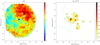 |
Fig. 2. Color spatial pattern in Haro 14. Left: (V − I) color index map; bluer colors indicate the bluer (younger) SF regions and red corresponds to the redder (older) stars in the galaxy. The map is not corrected for the contribution of emission lines. Right: increment in the (V − I) color index due to the contribution of emission lines. The blue line roughly delineates the bluish but not ionizing stellar component unveiled in the color map and the black contour corresponds to ΔL(V − I) = 0.01. |
A well-known problem when interpreting the broadband photometry of starbursts is the contamination by emission lines: the light from strong lines generated in the warm ionized gas adds to the flux in broadband filters and can significantly modify the integrated colors and color patterns of galaxies (Krueger et al. 1995; Zackrisson et al. 2001; Anders & Fritze-v. Alvensleben 2003; Cairós et al. 2002, 2007). Hence, a reliable photometry for the stellar component requires the quantification of the gas emission. As this gaseous contribution presents high spatial variability, the correction by means of traditional observing techniques is troublesome and observationally demanding: in addition to the broad-band frames, we need narrow-band imaging in each bright emission line or, alternatively, a sequence of long-slit spectra sweeping the starburst region. This, in turn, introduces uncertainties associated to the combination of frames taken with different instrumental setups and/or atmospheric conditions, or from the positioning of the slit (Guseva et al. 2001, 2003a,b; Guseva et al. 2003c, 2004; Cairós et al. 2007).
Integral field observations with MUSE overcome these problems in an efficient and precise manner. MUSE provides wide field imaging and spectroscopy simultaneously for every element of spatial resolution in a large spectral range. This offers several ways to get rid of the emission line contribution: we can generate images in the brightest lines and delimit the areas affected by gas; we can build color maps using galaxy images in spectral regions free of emission lines (the “pure continuum” maps presented in Sect. 2.5); and also, we can precisely quantify the contribution of the emission lines in each standard broadband filter.
That the blue color in the eastern sector of Haro 14 is intrinsic and not due to gas emission into the broadband filters can be readily proven from the analysis of the spatial distribution of emission lines. The emission line maps (see Sect. 3.5 below) clearly show that the ionized gas is concentrated in the central SF regions and its influence on the colors of the outer galaxy regions is minor. Furthermore, we generated color maps from pure continuum slices, that is, using spectral windows free from emission lines (see Sect. 2.5). We compared color maps with and without emission lines and find that, as expected, the nebular contribution is only important in the SF regions and the color spatial pattern remains the same in both cases.
We also computed the total flux of strong emission lines in every synthetic broadband filter and thus the contribution of the gas to the color maps. This is a simple task working with integral field data, which provide the full spectrum Fobs(λ) for each spatial resolution element. We obtained the flux, Fℓ(λ), due to the emission in the ℓ = 1, ..., Nℓ strongest lines by fitting their profiles (we considered here the two strongest recombination lines of H I and the [O III], [N II], and [S II] forbidden lines; Nℓ = 8 in all). The corrected flux for every element of spatial resolution is
which was then used to calculate the corrected synthetic colors and to derive the color increment due to emission lines, ΔEL(V − I). The color map corrected from emission lines can be directly obtained by adding the map of the increments to the original (V − I)obs map,

The right panel of Fig. 2 displays ΔEL(V − I) for Haro 14. Only the central SF regions are substantially affected by the ionized gas emission; whereas in the brighter knots ΔEL(V − I) is as high as 0.2, it is negligible outside of the SF regions. In particular, the blue region detected to the east is free of emission lines and its intrinsically blue color is a reliable indicator of an intermediate age stellar population.
Therefore, the color map of Haro 14 displays three well differentiated zones which trace three distinct stellar populations: the bluest knots in the inner part of the galaxy, which delineate the H II regions; the blue wide band extending northeast, which spatially coincides with the diffuse tail structure detected in continuum and has (V − I)∼0.5–0.7; and the redder areas in the outskirts with (V − I)∼0.8–1.0, which trace the LSB galaxy host. In addition to the unresolved stellar components, blobs with a broad range of colors are distinguished throughout the map, suggesting stellar clusters at different evolutionary stages.
Color maps are also useful to detect dust. In the (V − I) color map of Haro 14, we distinguish several red patches in the inner galaxy regions, quite prominent east and south-east of the central SF knots, that are likely due to dust. But without additional observational constrains, it is difficult to ascertain whether they trace dust or are just gaps in the blue stellar distribution.
3.4. Surface brightness photometry
Using the synthetic VRI images we also built the surface brightness profiles (SBPs) of Haro 14. Deriving the SBPs of irregular objects, such as BCGs, is not a straightforward task. The standard methods employed to perform surface brightness photometry, which assume some sort of galaxy symmetry, are not appropriate for describing the HSB regions of a BCG–this topic has been widely discussed in the literature and alternative procedures have been proposed (Papaderos et al. 1996, 2002; Doublier et al. 1997; Cairós et al. 2001b, 2003; Noeske et al. 2003; Gil de Paz & Madore 2005; Micheva et al. 2013a,b; Janowiecki & Salzer 2014).
We built the SBPs of Haro 14 following the approach described in Cairós et al. (2001a); Cairós et al. (2003). In the HSB regime, where the galaxy is markedly irregular, isophotal radial profiles are derived, that is, we compute the equivalent radii inside isophotes of decreasing intensity without making any assumptions about their geometrical shapes. In the outermost regions, we fit ellipses to the images using the IRAF task ellipse (Jedrzejewski 1987). The final SBP is created as a combination of these two profiles: the isophotal radial profiles in the high- and intermediate-intensity areas and elliptical fitting in the outer parts (see Fig. 3). In the central galaxy regions, the equivalent radius (Requiv) is defined as the radius of the circle whose area is equal to the corresponding isophotal surface; when fitting ellipses, the Requiv is computed as the square root of the product of the lengths of the semi-axes.
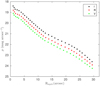 |
Fig. 3. Surface brightness profiles of Haro 14 built on the synthetic V, R, and I images from MUSE. |
The light profiles of Haro 14 do not show the most common behavior among BCGs, namely a brightness excess at high and intermediate intensity levels and a LSB host that is well described by an exponential function (Papaderos et al. 1996; Marlowe et al. 1997; Cairós et al. 2001b; Micheva et al. 2013a,b; Janowiecki & Salzer 2014). At intermediate radii, the profile displays a “plateau” or flattening, which is probably due to the blue and extended component that is well visible in the (V − I) color map. The LSB galaxy host cannot be fitted using a physically meaningful exponential, but the extrapolation of the fitted function to the central galaxy regions produces a higher surface brightness than that observed. Our SBPs are limited in radius by the MUSE FoV, but the more radially extended profiles derived in the optical (see Fig. 1 in Gil de Paz & Madore 2005) and in the NIR (Fig. 2 in Noeske et al. 2003) exhibit the same behavior out to a larger radius. Gil de Paz & Madore (2005) indeed fit an exponential function to the LSB host, but the derived fit has clearly no physical meaning (see their Fig. 1).
3.5. Emission line maps
The wide FoV and high sensitivity of MUSE allow for the detection of warm ionized gas emission out to large galactocentric distances (about 1.9–2.7 kpc) and very low surface brightness levels (∼4 × 10⁻²⁰erg s−1 cm−2 in Hα, per spaxel).
The intensity maps of Haro 14 in the brightest emission lines, Hα and [O III] λ5007, exhibit an intriguing morphology (Fig. 4). The inner galaxy areas are dominated by large H II regions, confirming the VIMOS results at a better spatial resolution (see Fig. 2 in CGP17a) while the current MUSE data reveal an intricate structure of bubbles, arcs, filaments, and faint blobs in the galaxy outskirts.
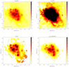 |
Fig. 4. Haro 14 maps in emission lines: Top-left: Hα emission line flux map of Haro 14; the chain-like structure and the curvilinear feature in the central regions are indicated with white lines. The blue line (bottom-left) corresponds to 1 kpc. Top-right: Hα emission line flux map with the intensity in the inner galaxy regions saturated in order to enhance the faint surface brightness features in the outer galaxy parts; the white lines indicate the most prominent shells and filaments in the galaxy periphery. Bottom-left: Hα equivalent width map (in Å); the blue line roughly delineates the bluish regions of the galaxy at intermediate intensity levels. Bottom-right: [O III] λ5007 flux map. Flux units in the emission line maps are 10−20 erg s−1 cm−2 (per spaxel); the central white cross marks the position of the galaxy peak in continuum. |
The copious H II regions indicate substantial and extended ongoing SF activity. The largest SF complexes are situated close to the central regions of the galaxy, forming a linear (chain-like) structure of about 1.8 kpc, roughly along the north–south direction, and in a horseshoe-like curvilinear feature, with a diameter of about 700 pc, which extends eastwards (see Fig. 4, top-left). Looking more carefully, we notice that the central SF chain-like structure is slightly curved, resembling incipient spiral arms. The emission in the galaxy periphery is dominated by LSB filaments and shells (see Fig. 4, top-right). Particularly impressive are the two curvilinear filaments extending southwest, highly detectable up to galactocentric distances of 2.0 and 2.3 kpc–such filaments extending far out into the halo are indicative that the galaxy is in an evolved phase of a starburst. A shell with a diameter of about 800 pc is clearly distinguished to the north and two smaller ones are visible departing southeast and northwest, respectively. Numerous faint knots appear scattered throughout the field, most of them in the vicinity of LSB structures. Also interesting are two emission blobs detached from the galaxy main body and highly visible to the west both in Hα and [O III].
The Hα and [O III] λ5007 maps are similar but some remarkable differences are present. First, the large filaments expanding southwest and the large bubble extending north, which are both highly visible in Hα, are not detected in [O III] λ5007–the same applies to other faint extensions. Second, the blobs visible on both maps do not necessarily coincide: several knots are only visible in one of the maps, and many of them are highly visible in one line but only marginally detected in the other. In general, the [O III] λ5007 emission appears more compact and more knotty.
3.6. Clumps in continuum and emission-line maps
Haro 14 exhibits numerous clumps spread out through the galaxy both in continuum and in emission-line maps. In continuum, three very bright knots sit roughly at the center of the HSB area and many fainter ones are evident at larger galactocentric distances, mostly clustered in the eastern galaxy regions (Fig. 1). In the emission line maps, the brightest clumps are placed along the central chain-like structure and in the horseshoe-like curvilinear feature extending eastwards, whereas fainter knots are visible in the surroundings (Fig. 4).
The clumps in emission lines are mainly H II regions and their ionizing stellar clusters. However, the nature of the sources detected in continuum is more difficult to asses: they could be groups of stars (e.g., stellar associations or clusters) or individual bright stars belonging to Haro 14, background galaxies, or foreground stars in the Milky Way (Leitherer et al. 1996; Östlin et al. 1998; Johnson et al. 2000). Their spatial distribution (the majority of the clumps are gathered in the blue area to the east) suggests that most of them indeed belong to Haro 14. In order to gain insight into the nature of these clumps, we derived their physical parameters–their sizes, magnitudes, and colors.
3.6.1. Source selection
The first step towards deriving the physical parameters of the sources is their detection and spatial delimitation. To this aim, we wrote a routine that automatically searches for clumps in both the continuum and the emission line maps. The characteristics of these maps are quite distinct: while the line maps have a higher contrast, that is, the local background is dim compared to the sources, in the continuum frames the local background may be very bright and fluctuating. We developed an algorithm able to work efficiently with both types of images.
Our routine does not make a priori assumptions about the size or shape of the sources, it can detect extended and noncircular features. The method selects a source by expanding from a local emission maximum until it makes contact with a nearby region or merges into the background. The algorithm consists of three steps: detection of the local maxima, iterative growth of the region, and stopping criteria.
-
Detection of the local maxima. The routine starts smoothing the image with a Gaussian filter (FWHM = 3 pixels). We then search for local maxima in this smoothed image. The flux of the local maxima has to be above the local background by some given threshold which depends on the noise characteristic of the frame. For this task, we adapted the routine FastPeakFind.m from the MATLAB Central File Exchange1. We end up with a list with the positions of the local maxima.
-
Iterative growth of the sources. For a given maximum, we started seeding a region with all the pixels around it with a flux above 95% of the peak–typically, between 4 and 15 pixels. Now, we proceed iteratively following a strategy similar to the HIIphot routine (Thilker et al. 2000). We begin defining the threshold, Ft, as the highest flux of the whole frame, which is then decreased by 1% in each step of the iteration. We incorporate to each source the pixels of its external perimeter (see below) with fluxes above the Ft, as long as they have not been incorporated to some other source. We distinguish between an external perimeter and an internal perimeter. The internal perimeter contains those pixels that belong to the source and are in contact with the current boundary and the external perimeter is composed of those pixels in contact with the boundary but not belonging to the source. In each step of the iteration, we search for pixels in the external perimeter of each region whose flux is above the flux threshold and are not claimed by other sources. A problem with this strategy, and particularly relevant for continuum images, appears when there is a gradient on the underlying background, in which case the selected region may grow incorrectly along the background gradient. To alleviate this, we forced the number of pixels added to the region to be at least 30% of those in the external perimeter and their fluxes to be lower than the median of the internal perimeter. We only consider pixels whose distance to the center of the region, di, verifies

where D is the median of the distance to the center of the pixels in the internal perimeter of the region and fe is an input parameter that prevents excessive elongation of the sources. We set fe = 1.25 for the catalog of features detected in continuum and fe = 1.50 for those detected in emission lines. This difference arises from the fact that the H II regions are expected to be larger and less round than continuum features.
-
Stopping criteria. A region ceases to grow when no more pixels satisfying the above criteria can be added to the region, the surface brightness profile flattens, or the region comes into contact with another adjacent source. The surface brightness profile has flattened when
where ⟨Fext⟩ and ⟨Finter⟩ are the flux averages of the external and internal perimeters, respectively, and fflat is an input parameter (we adopted fflat = 0.97 in this work). Also, we require that the flux average of the external and the internal perimeters decrease with each iteration i (i.e., ⟨Fext, i⟩< ⟨Fext, i − 1⟩;⟨Fint, i⟩< ⟨Fint, i − 1⟩). When two adjacent regions are in contact by more than two pixels, the growth of both is stopped to avoid the contamination of one source by the other. In addition, we impose two other conditions to avoid the growth of the sources to unrealistic sizes. First, only pixels with a flux above 15% of the flux of the region peak can be added to the source. Second, we fix an upper bound for a source size: 100 pixels for the continuum sources and 150 pixels for the emission line regions.
The routine provides the list of identified sources, their spatial position, and a mask with the pixels belonging to each source, together with a series of parameters helping to control the operation of the algorithm.
3.6.2. Background subtraction
An important albeit difficult step in the characterization of the sources is the subtraction of the background. The clumps we identified lie on top of unresolved stellar and gaseous emission, and therefore to extract their intrinsic flux, we must first subtract the light contribution coming from the underlying components. This is a complicated task because the background is highly inhomogeneous, which prevents a global modelling. Also, we are interested in extracting the intrinsic spectrum of the region in the whole spectral range and not merely in the photometry of the sources in specific filters, meaning that traditional techniques are not immediately applicable here.
We determine the local background per pixel for each source individually, as the median of the spectra of the pixels in a region around the source. We select this region as a strip of two pixels in width, two pixels away from the boundary as a compromise in order to get a good signal-to-noise ratio (S/N) spectrum while minimizing contamination from the source. We exclude pixels belonging to nearby regions from the background strip.
3.6.3. Determination of the parameters of the sources
From the background-subtracted data, we determined the spatial properties of the sources. The center of the source is located at the centroid of its pixels (i.e., the intensity-weighted means of the marginal profiles in the X and Y directions of all pixels of the source). The area is simply the area of the pixels belonging to the source. However, this value may not be a good characterization of the actual extension of the region because it could be affected by background inhomogeneities or gradients (see discussion above, Sect. 3.6.1). A better measure of the size of the source is its FWHM, which we calculate here as the equivalent diameter of the region formed by all the pixels with a flux larger than half the maximum value.
The integrated spectrum of each individual blob is generated by adding the spectra of its corresponding spaxels and removing the local background (see above). We then calculate the fluxes in the brighter emission lines (lines are fitted as described in Sect. 2.5).
The intrinsic (background-subtracted) photometry in the VRI filters was generated from flux maps. The intrinsic inhomogeneity of the underlying galaxy and the systematic errors of the instrument are the dominant factor in the photometric error budget, much larger than the photonic noise (if the background were uniform and the observations photon limited, photometric errors would be well below 0.01 mag). These sources of error are also highly correlated from filter to filter. We estimate the uncertainty due to the background subtraction as the standard deviation of the fluxes in the strip around the source divided by the square root of the number of pixels. From this we calculate the corresponding errors in the magnitudes. For most sources, V is determined with a precision of a few hundredths of a magnitude (see Table 3). The few sources with higher values have highly inhomogeneous surroundings for which a background estimate is therefore more uncertain. The uncertainties on the colors are reduced with respect to a simple quadratic sum of the broadband errors because of the covariance of the correlated noise.
Properties of the continuum sources detected in Haro 14.
3.6.4. Catalogs of continuum and emission line sources
We ran the routine for source detection in two continuum maps, one in the blue spectral region (5400–5600 Å) and one in the red (7800–8000 Å), and found 42 and 38 objects, respectively. These sources could be objects belonging to Haro 14 (stellar groups or individual bright stars), foreground Galactic stars, or background galaxies.
In order to discriminate among the distinct possibilities we used the integrated spectra of the individual sources. This way, we discovered two background galaxies (see Fig. 2 and Appendix A) and eliminated from the catalog several blobs with poor S/N spectrum for which a reliable redshift could not be determined. All remaining clumps are at the same redshift as Haro 14–there are no foreground stars in the field.
The final catalog contains 29 sources that undoubtedly belong to Haro 14–all of them were detected by the routine in both the blue and the red map. Their position, area, FWHM, and photometry are presented in Table 3. Figure 5 (upper left panel) shows that their distribution is not uniform through the galaxy, but most of them gather on the eastern sector.
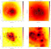 |
Fig. 5. Clumps detected in Haro 14. Top-left: the 29 sources (clumps) detected in continuum (see also Table 3) overplotted on the blue (5400–5600 Å) continuum map. There is an evident clustering of the clumps at the galaxy eastern regions. Top-right: zoom into the central 20″ × 20″. The flux units are arbitrary. Bottom-left: the 55 clumps detected in emission lines (see also Table 4) overplotted on the Hα map; sources detected in Hα and [O III] λ5007 appear in blue, sources detected only in Hα in cyan, and those detected only in [O III] λ5007 in green. Bottom-right: zoom into the central galaxy regions. The intensity scale is logarithmic and the cross marks the position of the continuum peak. |
Of the 29 sources, 18 are extended (we consider extended sources those with FWHM ≥ 1″) and are therefore definitely groups of stars (e.g., H II-regions complexes or stellar associations). Point-like objects may still be unresolved stellar groups or individual stars. Using the photometry we can further constrain their nature: adopting an absolute magnitude MV = −8.5 as the cutoff for single stars (Whitmore et al. 1999; Johnson et al. 2000), we conclude that the four point-like sources brighter that this limit are also not individual stars, but complexes of stars. Source C19, with (V − I) = 2.34, is likely a red supergiant (RSG), as sources with (V − I)≥1.50 can be safely classified as stars (Whitmore et al. 1995; Miller et al. 1997; Harris 1996, 2010 edition), but the nature of the remaining six point-like sources cannot be unequivocally established using only photometrical criteria.
We also ran our routine in the emission lines maps. We detected 41 sources in Hα and 41 in [O III] λ5007; of these, 30 sources appear in both lines, 12 only in Hα, and 13 only in [O III] λ5007, which gives a total of 55 individual sources. Objects detected in emission lines are most likely SF regions; although some of them could also be supernova remnants (SNRs; Osterbrock et al. 2006; Vučetić et al. 2013, 2015, 2019). Only six of these sources have a clear counterpart in the continuum and they are identified as HII in Table 3.
The main properties of the emission sources are presented in Table 4. Figure 5 (lower left panel) shows that, by contrast with the continuum ones, their distribution is more homogeneous through the central part of the galaxy. Nearly all sources are extended–90% have FWHM larger than 1 arcsec (63 pc)–, hence, they are relatively large H II-region complexes, and span a wide range in fluxes and luminosities, with Hα luminosity varying from LHα = 1034.3–1038.9 erg s−1. Most objects present luminosities typical of classical H II regions (LHα ≤ 1037 erg s−1), whereas roughly 30% can be classified as giant H II regions2 (GHIIR; LHα = 1037–1039 erg s−1). The flux of recombination lines is proportional to the number of photons emitted above the Lyman continuum and therefore to the number of ionizing stars. Regions with luminosities LHα < 1037 erg s−1 are ionized by one or several stars, while GHIIRs must be ionized by multiple associations or stellar clusters. We note that the values shown in Table 4 are not corrected for interstellar extinction: the de-reddened fluxes are somewhat larger. Applying, for instance, the value of the interstellar extinction coefficient derived in CGP17a for the integrated spectrum of Haro 14, C(Hβ) = 0.379, we would derive fluxes twice as large as the tabulated ones. However, large spatial variations of the extinction are expected in Haro 14, meaning that an accurate interstellar extinction correction must be done in two dimensions.
Properties of the emission-line sources detected in Haro 14.
The detailed analysis of the properties of the individual sources detected both in continuum and in emission line maps is out of the scope of this paper and will be presented in a forthcoming publication (Cairós et al., in prep.)
4. Discussion
The huge amount of information contained in the MUSE data enabled us to conduct a thorough analysis of the BCG Haro 14. The unique combination of high spatial resolution, wide FoV, and extended wavelength coverage mean that MUSE is a powerful tool with which to disentangle the distinct stellar populations and, in particular, to fully characterize the ongoing starburst. This is the first step towards establishing the evolutionary status of the galaxy and deriving its star forming history (SFH). In addition, an accurate depiction of the properties of the young stars (spatial position, ages and metallicities) may provide insights into the mechanism(s) that triggers and controls the SF activity.
4.1. First view on the stellar populations
Like most BCGs, Haro 14 harbors an inner, mostly line-emitting HSB region embedded in a LSB stellar host (Marlowe et al. 1997; Doublier et al. 1999; Noeske et al. 2003; Gil de Paz et al. 2003). The large FoV of MUSE allowed us to perform accurate spectrophotometry for both the HSB and the LSB area: we were able to investigate the stellar component in the galaxy outskirts, which are free from the contribution of young stars and gas, as well as to resolve filaments of ionized gas and faint H II-regions up to kiloparsec scales. This is a decisive asset with respect to previous IFS BCG studies, which, due to their limited FoV, could only cover the central HSB area, or in most cases merely a fraction of it (Vanzi et al. 2008, 2011; García-Lorenzo et al. 2008; Cresci et al. 2010; Kehrig et al. 2008, 2013; Cairós et al. 2009a,b; Cairós & González-Pérez 2017a,b, 2020; James et al. 2010, 2013a, b; Lagos et al. 2018; Kumari et al. 2017, 2019).
The comparison of Haro 14 continuum and emission line maps generated our first interesting results (Figs. 1 and 4). Continuum and line maps exhibit very distinct morphologies, the most evident difference being found in the outer galaxy regions: the stellar component shows a regular LSB envelope, while in ionized gas the faint intensity regions appear highly irregular and mostly made of filaments, shells, loops, and arcs. This is indeed what is found in the vast majority of BCGs, a dynamically relaxed stellar host underlying a star-forming population (Loose & Thuan 1986; Marlowe et al. 1997; Beck & Kovo 1999; Cairós et al. 2001a; Gil de Paz et al. 2003).
In Haro 14, however, the spatial patterns of the stars and ionized gas are also markedly different at high and intermediate intensity levels. At HSB, the continuum shows a main peak and two subsidiary ones within a radius of ∼300 pc (knots 1, 2 and 3, top panels in Fig. 5), while the gas emission is clumpy and extended (the maxima in gas emission spread up to kiloparsec scales; see Fig. 5, bottom panels). None of the three major continuum emitters spatially coincides with a peak in emission lines, indicating that they are relatively evolved (nonionizing) stellar clusters or associations.
At intermediate brightness levels, the morphology of Haro 14 is intriguing: in the continuum maps, the intensity decreases unevenly, and we distinguish a diffuse structure extending northeast (Fig. 1). This structure is also evident in the SBPs of the galaxy as a flattening between 0.9 and 1.6 kpc (Fig. 3). In the color maps, it appears as a band with intrinsic blue colors that occupies most of the eastern galaxy region.
Combining the information from the color and the galaxy maps, we identify three different stellar populations:
-
A very young stellar component, depicted in the emission line maps–only rapidly evolving OB stars (ages≤10 Myr) produce photons energetic enough to ionize hydrogen (Leitherer & Heckman 1995; Ekström et al. 2012; Langer 2012). This current starburst presents a highly irregular morphology, takes place in numerous SF complexes, and is considerably extended: H II-regions are detected over the whole FoV up to galactocentric distances of ∼1.8 kpc.
-
An intermediate-age component, whose presence is suggested by the pure continuum maps (Fig. 1, right panels) and is confirmed by the color (Fig. 2, left panel) and Hα equivalent-width maps (Fig. 4 bottom left). The continuum frames exhibit an irregular and diffuse appearance in the eastern galaxy regions, which points to a population of stars in a nonequilibrium state. In the color index map, this area is visible as a wide band with blue colors (V − I ∼ 0.5−0.7), characteristic of young stars, while the Hα equivalent-width map in this region shows very low values (W(Hα) ≤ 10Å), proving that ionizing stars have already evolved–which clearly distinguishes this stellar population from the ongoing starburst. According to evolutionary synthesis models, such blue colors are consistent with a stellar population with ages of between 10 and 300 Myr (Fioc & Rocca-Volmerange 1997; Leitherer et al. 1999; Bruzual & Charlot 2003).
-
An extended LSB component, whose red colors and smooth, almost round shape are indicative of an old, relaxed stellar population. The comparison of the colors with evolutionary synthesis models (Vazdekis et al. 1996, 2010; Fioc & Rocca-Volmerange 1997; Le Borgne et al. 2004) suggests ages of several Gyr, which is in agreement with the values derived by Noeske et al. (2003) and Marlowe et al. (1997).
4.2. Stellar complexes in Haro 14
In addition to the unresolved stellar components in Haro 14, we detected many clumps scattered through the galaxy, most of which we identified as stellar complexes (i.e., H II-regions, stellar clusters, or stellar associations) in Sect. 3.6.4. A detailed analysis of the individual H II-regions, clusters, and associations by means of spectral synthesis techniques to determine their masses, extinction, metallicities, and ages will be presented in a forthcoming publication. Here we advance some preliminary results on the properties of these individual stellar groups based mainly on their photometry.
The H II regions identified in the emission line maps belong evidently to the ongoing starburst. Using the Hα equivalent width we can further constrain their ages. The most luminous SF regions all present W(Hα)≥100 Å (see Fig. 4 bottom left); according to STARBURST 99 synthesis models (Leitherer et al. 1999) this translates into ages ≤6.3 Myr –adopting the models with metallicity z = 0.008, the closest value to the metallicity derived from the emission-line fluxes (CGP17a). These ages must be understood, however, as an upper limit, as the measured equivalent widths can decrease as a result of absorption from A-F stars and/or dilution due to the continuum from an older stellar population (Fernandes et al. 2003; Levesque & Leitherer 2013).
By contrast, the sources detected in continuum are very different regarding their ages and evolutionary paths, ranging from complexes of very young stars still embedded in their natal clouds to ancient globular clusters. The first hint as to their diversity is provided by the large variations in magnitudes and colors they present (Table 3 and Fig. 6). Absolute magnitudes vary from MV = −6.70 to MV = −12.18, while the color index (V − I) changes from very blue (−0.12) to quite red (1.06)–we have excluded here source C19 identified as a RSG in Sect. 3.6.4. Six stellar complexes show blue colors, are co-spatial with (or very close to) an emission line source, and have H II-like spectra: these are the clusters or associations that are rich in ionizing stars and create the H II regions. Five clumps are red, with colors–V − I ≥ 0.8–characteristic of intermediate age or old globular clusters. Most of the sources have intermediate colors in the range 0.2 ≤ (V − I)≤0.8 and no counterpart in emission lines. These young but nonionizing stellar complexes are gathered in the eastern regions of the galaxy, in the blue zone that is highly visible in the color map, and display similar blue colors. They are probably stellar clusters and/or associations in the process of dissolution.
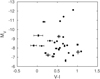 |
Fig. 6. MV vs. (V − I) color–magnitude diagram for the sources identified in the continuum maps of Haro 14. |
The majority of the stellar complexes detected in Haro 14 are extended, that is, they are large H II regions or stellar associations. Among the point-like objects, the two most luminous, C1 and C3, display properties consistent with those of super stellar clusters (SSCs). In particular, the continuum peak, C1, situated in the inner galaxy regions and having MV = −12.18, is definitely a very strong SSC candidate. In CGP17a, we used the equivalent widths in absorption of the higher order Balmer lines to constrain the age of the continuum peak and found values of between 10 and 30 Myr. This points to a young age for the SSC candidate C1– young ages and red colors together could be naturally explained by the presence of RSGs.
Super stellar clusters are extremely compact and luminous objects thought to be created in violent episodes of SF (Arp & Sandage 1985; Holtzman et al. 1996; Ho 1997). Their characteristics make them particularly interesting in the context of extragalactic research: because they are bright they can be observed at large distances, and because they are long lived, they retain valuable information on the SFH of their host galaxies (Larsen 2010; Portegies Zwart et al. 2010; Adamo et al. 2020).
4.3. The trigger mechanism of SF in Haro 14
An important open question in BCG research is which mechanism triggers such violent episodes of SF in (apparently) isolated systems (Pustilnik et al. 2001; Brosch et al. 2004; Hunter & Elmegreen 2006; Elmegreen et al. 2012). We find evidence of at least two different SF episodes in Haro 14: the ongoing starburst, with ages of about 6 Myr, and a previous episode of SF, a precursor to the irregular and blue population observed in the continuum frames and color maps, which ignited from ten to several hundred million years ago. We proposed in CGP17a that the current starburst was triggered by an earlier (star-induced) SF episode, that is, as the effect of the collective action of stellar winds and supernova originated in a previous burst, seemingly ten to thirty million years ago. However, the mechanism responsible for the onset of that previous starburst remains unclear.
The findings presented here point to mergers or interactions as a plausible explanation: a pronounced asymmetry in the stellar distribution, such as that seen in Haro 14, is a common feature in galaxy pairs and merger systems (Conselice 2003; Zheng et al. 2004; Hernández-Toledo et al. 2005; De Propris et al. 2007; Ellison et al. 2010; Xu et al. 2020); tail structures, such as the one observed in the northeast regions of Haro 14 (see Fig. 2), also appear as the result of interactions (Toomre & Toomre 1972; Mullan et al. 2011; Struck 2011; Duc & Renaud 2013); and the possible detection of SSCs suggests at least one episode of violent SF in the past, as such massive clusters require large quantities of gas infalling in a small region (high-pressure environments) in a short time interval (Whitmore et al. 2003; Dobbs et al. 2020).
Our results are in line with an increasing amount of observational evidence suggesting that interactions (Brinks 1990; Taylor et al. 1996; Östlin et al. 2001; Pustilnik et al. 2001) or external infalling gas (López-Sánchez et al. 2012; Nidever et al. 2013; Ashley et al. 2014; Miura et al. 2015; Turner et al. 2015) do indeed play a major role in the ignition of the starburst in low-mass systems. In particular, observational evidence of mergers between dwarf galaxies has grown considerably in recent years (Martínez-Delgado et al. 2012; Paudel et al. 2015, 2018; Privon et al. 2017; Zhang et al. 2020a,b). This opens a very interesting line of research, as mergers and interactions in nearby BCGs provide an excellent chance to probe the hierarchical scenario in conditions very similar to those found in the high-redshift Universe, at the epoch of galaxy formation.
5. Summary and conclusions
This is the first in a series of papers presenting results from a MUSE/VLT-based study of the BCG Haro 14. MUSE provides integral field data in a large wavelength range (4750–9300 Å), with high spatial resolution and unprecedented sensitivity. Moreover, its large FoV (1′×1′ = 3.8 × 3.8 kpc2) enables accurate spectroscopy to be obtained not only in the central starburst region but also in the LSB galaxy component.
We performed an exhaustive investigation of the morphology, structure, and stellar populations of Haro 14. We built continuum maps in several spectral regions free of strong emission lines (e.g., 5400–5600 Å and 7800–8000 Å) as well as in the brightest emission lines (Hα and [O III] λ5007). We also generated synthetic broad-band images in the VRI bands of the Johnson-Cousins UBVRI system, from which we produced color index maps and SBPs. We detected numerous discrete sources (clumps) spread out through the galaxy, both in continuum and in emission lines. We developed a routine that searches for these sources automatically and produced a final catalog with their positions, sizes, and photometry.
From our analysis we highlight the following results:
-
The stellar distribution of Haro 14 is markedly asymmetric. In continuum maps free from line emission, the intensity peak is not centered with respect to the LSB host, but displaced by ∼500 pc southwest; from there, the intensity decreases unevenly, with galaxy isophotes clearly elongated in the northeast direction. We identify a stellar structure resembling a tail, extending about 1.9 kpc northeast, which likely traces a nonrelaxed stellar component.
-
The galaxy color maps reveal a blue, but nonionizing stellar component, which covers almost the whole eastern part of the galaxy. This blue component extends to kiloparsec scales and largely overlaps with the tail structure detected in the continuum maps.
-
We identified (at least) three different stellar populations in Haro 14: an ongoing starburst, a young but nonionizing stellar population, and the extended LSB host. The recent starburst is composed of a large number of H II-region complexes distributed all over the galaxy main body; the brightest H II regions have ages of about 6 Myr. The highly irregular, blue but nonionizing stellar component dominates the emission in the eastern part of the galaxy, and shows observables consistent with ages of between ten and several hundred million years. Finally, the LSB host is a red and regular-shaped component of several gigayears.
-
In addition to the unresolved stellar components, we also identify a large number of discrete sources in the galaxy: 55 in emission line maps and 29 in the continuum–only 6 belonging to both groups. The gas emission sources are most likely H II regions. The sources in the continuum include, along with the six ionizing groups associated with H II regions, at least 16 other stellar complexes in different evolutive stages. The two most luminous ones have properties consistent with SSCs, in particular the continuum peak (Mv = −12.18) is a strong SSC candidate.
The striking asymmetry of the stellar distribution in Haro 14 in continuum maps, the highly irregular blue stellar population detected in the color map, the anomalous behavior of its SBP which cannot be described by a simple law even at large radii, and the presence of numerous stellar complexes, some of them young massive and super stellar cluster candidates, speak in favor of the possibility that interactions or mergers have taken place in Haro 14. This is indeed an appealing hypothesis, as interactions or mergers in nearby, low-mass, metal-poor starburst systems would provide an excellent opportunity to probe the hierarchical scenario in conditions very similar to those found in the early Universe. In a forthcoming publication, we shall explore the interaction or merger scenario with results from a kinematical analysis of the MUSE data.
Studies focused on the stellar content and SFH of low-mass metal-poor starbursts are crucial for understanding galaxy formation and evolution. It is particularly important to determine the recent SFH in these objects, as this contains valuable information on the impact of massive stellar feedback within a low gravitational potential, and on the mechanism that ignites the burst. Detailed studies on the SFH of BCGs are unfortunately scarce: the color–magnitude diagram (CMD) synthesis method can be applied only to nearby systems (Tolstoy et al. 2009) and BCGs are rare objects; only a handful are close enough to be resolved into stars (Lee et al. 2009; Karachentsev & Kaisina 2019). The few BCGs analyzed by means of CMD methods indeed show a complex and varied recent SFH–e.g., VII Zw 403 (Schulte-Ladbeck et al. 1999a,b); Mrk 178 (Schulte-Ladbeck et al. 2000); NGC 1705 (Annibali et al. 2003, 2009); NGC 5253 (Davidge 2007; McQuinn et al. 2010); UGC 4483 (Izotov & Thuan 2002; McQuinn et al. 2010; Sacchi et al. 2021). This emphasizes the importance of determining the SFH in a large and representative sample of low-mass starbursts.
The present work shows that integral field spectroscopy provides an excellent alternative technique with which to investigate the stellar populations and SFH of galaxies that cannot be resolved into stars. In particular, the presently unique capabilities of MUSE, namely its wide FoV, large spectral range, and high spatial resolution, play a decisive role in investigations of the stellar populations and SFHs of dwarf star-forming galaxies.
Natan (2020). Fast 2D peak finder (https://www.mathworks.com/matlabcentral/fileexchange/37388-fast-2d-peak-finder), MATLAB Central File Exchange.
As a reference, Orion, with a diameter of about 5 pc and L(Hα) = 1.0 × 1037 erg cm−1 is a classical H II-region, while 30 Dor, which has a diameter of about 200 pc and L(Hα) = 1.5 × 1040 erg s−1 is a super giant H II-region (Kennicutt 1984).
Acknowledgments
L. M. C acknowledges support from the Deutsche Forschungsgemeinschaft (CA 1243/1-1 and CA 1234/1-2). P. M. W. received support from BMBF Verbundforschung (project MUSE-NFM, grant 05A17BAA). Based on observations collected at the European Southern Observatory under ESO programme ID 60.A-9186(A). This research has made use of the NASA/IPAC Extragalactic Database (NED), which is operated by the Jet Propulsion Laboratory, Caltech, under contract with the National Aeronautics and Space Administration. We acknowledge the usage of the HyperLeda database (http://leda.univ-lyon1.fr). This work also used IRAF package, which are distributed by the National Optical Astronomy Observatory, which is operated by the Association of Universities for Research in Astronomy, Inc., under contract with the National Science Foundation.
References
- Adamo, A., Zeidler, P., Kruijssen, J. M. D., et al. 2020, Space Sci. Rev., 216, 69 [Google Scholar]
- Aller, L. H. 1984, Physics of Thermal Gaseous Nebulae (Astrophysics and Space Science Library) [Google Scholar]
- Anders, P., & Fritze-v Alvensleben, U. 2003, A&A, 401, 1063 [NASA ADS] [CrossRef] [EDP Sciences] [Google Scholar]
- Annibali, F., Greggio, L., Tosi, M., Aloisi, A., & Leitherer, C. 2003, AJ, 126, 2752 [NASA ADS] [CrossRef] [Google Scholar]
- Annibali, F., Tosi, M., Monelli, M., et al. 2009, AJ, 138, 169 [NASA ADS] [CrossRef] [Google Scholar]
- Arp, H., & Sandage, A. 1985, AJ, 90, 1163 [NASA ADS] [CrossRef] [Google Scholar]
- Ashley, T., Elmegreen, B. G., Johnson, M., et al. 2014, AJ, 148, 130 [NASA ADS] [CrossRef] [Google Scholar]
- Bacon, R., Accardo, M., Adjali, L., et al. 2010, in Ground-based and Airborne Instrumentation for Astronomy III, Proc. SPIE, 7735, 773508 [Google Scholar]
- Bassino, L. P., & Caso, J. P. 2017, MNRAS, 466, 4259 [NASA ADS] [Google Scholar]
- Beck, S. C., & Kovo, O. 1999, AJ, 117, 190 [NASA ADS] [CrossRef] [Google Scholar]
- Bessell, M. S. 1990, PASP, 102, 1181 [NASA ADS] [CrossRef] [Google Scholar]
- Bessell, M. S., Castelli, F., & Plez, B. 1998, A&A, 333, 231 [NASA ADS] [Google Scholar]
- Bik, A., Östlin, G., Hayes, M., et al. 2015, A&A, 576, L13 [NASA ADS] [CrossRef] [EDP Sciences] [Google Scholar]
- Bik, A., Östlin, G., Menacho, V., et al. 2018, A&A, 619, A131 [NASA ADS] [CrossRef] [EDP Sciences] [Google Scholar]
- Brinks, E. 1990, in II Zwicky 33: star formation induced by a recent interaction, ed. R. Wielen, 146 [Google Scholar]
- Brosch, N., Almoznino, E., & Heller, A. B. 2004, MNRAS, 349, 357 [NASA ADS] [CrossRef] [Google Scholar]
- Bruzual, G., & Charlot, S. 2003, MNRAS, 344, 1000 [NASA ADS] [CrossRef] [Google Scholar]
- Cairós, L. M., & González-Pérez, J. N. 2017a, A&A, 600, A125 [NASA ADS] [CrossRef] [EDP Sciences] [Google Scholar]
- Cairós, L. M., & González-Pérez, J. N. 2017b, A&A, 608, A119 [NASA ADS] [CrossRef] [EDP Sciences] [Google Scholar]
- Cairós, L. M., & González-Pérez, J. N. 2020, A&A, 634, A95 [NASA ADS] [CrossRef] [EDP Sciences] [Google Scholar]
- Cairós, L. M., Caon, N., Vílchez, J. M., González-Pérez, J. N., & Muñoz-Tuñón, C. 2001a, ApJS, 136, 393 [CrossRef] [Google Scholar]
- Cairós, L. M., Vílchez, J. M., González Pérez, J. N., Iglesias-Páramo, J., & Caon, N. 2001b, ApJS, 133, 321 [CrossRef] [Google Scholar]
- Cairós, L. M., Caon, N., García-Lorenzo, B., Vílchez, J. M., & Muñoz-Tuñón, C. 2002, ApJ, 577, 164 [CrossRef] [Google Scholar]
- Cairós, L. M., Caon, N., Papaderos, P., et al. 2003, ApJ, 593, 312 [CrossRef] [Google Scholar]
- Cairós, L. M., Caon, N., García-Lorenzo, B., et al. 2007, ApJ, 669, 251 [CrossRef] [Google Scholar]
- Cairós, L. M., Caon, N., Papaderos, P., et al. 2009a, ApJ, 707, 1676 [CrossRef] [Google Scholar]
- Cairós, L. M., Caon, N., Zurita, C., et al. 2009b, A&A, 507, 1291 [NASA ADS] [CrossRef] [EDP Sciences] [Google Scholar]
- Cairós, L. M., Caon, N., Zurita, C., et al. 2010, A&A, 520, A90 [NASA ADS] [CrossRef] [EDP Sciences] [Google Scholar]
- Cairós, L. M., Caon, N., García Lorenzo, B., et al. 2012, A&A, 547, A24 [NASA ADS] [CrossRef] [EDP Sciences] [Google Scholar]
- Cairós, L. M., Caon, N., & Weilbacher, P. M. 2015, A&A, 577, A21 [NASA ADS] [CrossRef] [EDP Sciences] [Google Scholar]
- Calzetti, D., Conselice, C. J., Gallagher, J. S. I., & Kinney, A. L. 1999, AJ, 118, 797 [NASA ADS] [CrossRef] [Google Scholar]
- Calzetti, D., Harris, J., Gallagher, J. S. I., et al. 2004, AJ, 127, 1405 [NASA ADS] [CrossRef] [Google Scholar]
- Chisholm, J., Tremonti, C., & Leitherer, C. 2018, MNRAS, 481, 1690 [NASA ADS] [CrossRef] [Google Scholar]
- Conselice, C. J. 2003, ApJS, 147, 1 [NASA ADS] [CrossRef] [Google Scholar]
- Cresci, G., Vanzi, L., Sauvage, M., Santangelo, G., & van der Werf, P. 2010, A&A, 520, A82 [NASA ADS] [CrossRef] [EDP Sciences] [Google Scholar]
- Cresci, G., Vanzi, L., Telles, E., et al. 2017, A&A, 604, A101 [NASA ADS] [CrossRef] [EDP Sciences] [Google Scholar]
- Davidge, T. J. 2007, AJ, 134, 1799 [NASA ADS] [CrossRef] [Google Scholar]
- Davies, R. I. 2007, MNRAS, 375, 1099 [Google Scholar]
- Dekel, A., & Silk, J. 1986, ApJ, 303, 39 [Google Scholar]
- De Propris, R., Conselice, C. J., Liske, J., et al. 2007, ApJ, 666, 212 [NASA ADS] [CrossRef] [Google Scholar]
- de Vaucouleurs, G., de Vaucouleurs, A., Corwin, Jr., H. G., et al. 1991, in Third Reference Catalogue of Bright Galaxies [Google Scholar]
- De Young, D. S., & Heckman, T. M. 1994, ApJ, 431, 598 [NASA ADS] [CrossRef] [Google Scholar]
- Dobbs, C. L., Liow, K. Y., & Rieder, S. 2020, MNRAS, 496, L1 [NASA ADS] [CrossRef] [Google Scholar]
- Doublier, V., Comte, G., Petrosian, A., Surace, C., & Turatto, M. 1997, A&AS, 124, 405 [NASA ADS] [CrossRef] [EDP Sciences] [Google Scholar]
- Doublier, V., Caulet, A., & Comte, G. 1999, A&AS, 138, 213 [NASA ADS] [CrossRef] [EDP Sciences] [Google Scholar]
- Doublier, V., Caulet, A., & Comte, G. 2001, A&A, 367, 33 [NASA ADS] [CrossRef] [EDP Sciences] [Google Scholar]
- Duc, P. A., & Renaud, F. 2013, in Tides in Colliding Galaxies, eds. J. Souchay, S. Mathis, & T. Tokieda, 861, 327 [Google Scholar]
- Ekström, S., Georgy, C., Eggenberger, P., et al. 2012, A&A, 537, A146 [Google Scholar]
- Ellison, S. L., Patton, D. R., Simard, L., et al. 2010, MNRAS, 407, 1514 [NASA ADS] [CrossRef] [Google Scholar]
- Elmegreen, B. G., Zhang, H.-X., & Hunter, D. A. 2012, ApJ, 747, 105 [NASA ADS] [CrossRef] [Google Scholar]
- Fernandes, R. C., Leão, J. R. S., & Lacerda, R. R. 2003, MNRAS, 340, 29 [NASA ADS] [CrossRef] [Google Scholar]
- Fioc, M., & Rocca-Volmerange, B. 1997, A&A, 500, 507 [NASA ADS] [Google Scholar]
- Fukugita, M., Ichikawa, T., Gunn, J. E., et al. 1996, AJ, 111, 1748 [Google Scholar]
- García-Lorenzo, B., Cairós, L. M., Caon, N., Monreal-Ibero, A., & Kehrig, C. 2008, ApJ, 677, 201 [CrossRef] [Google Scholar]
- Garnett, D. R. 2002, ApJ, 581, 1019 [NASA ADS] [CrossRef] [Google Scholar]
- Gil de Paz, A., & Madore, B. F. 2005, ApJS, 156, 345 [NASA ADS] [CrossRef] [Google Scholar]
- Gil de Paz, A., Madore, B. F., & Pevunova, O. 2003, ApJS, 147, 29 [NASA ADS] [CrossRef] [Google Scholar]
- González Delgado, R. M., & Leitherer, C. 1999, ApJS, 125, 479 [CrossRef] [Google Scholar]
- González Delgado, R. M., Leitherer, C., & Heckman, T. M. 1999, ApJS, 125, 489 [CrossRef] [Google Scholar]
- Gordon, D., & Gottesman, S. T. 1981, AJ, 86, 161 [NASA ADS] [CrossRef] [Google Scholar]
- Guseva, N. G., Izotov, Y. I., Papaderos, P., et al. 2001, A&A, 378, 756 [NASA ADS] [CrossRef] [EDP Sciences] [Google Scholar]
- Guseva, N. G., Papaderos, P., Izotov, Y. I., et al. 2003a, A&A, 407, 75 [NASA ADS] [CrossRef] [EDP Sciences] [Google Scholar]
- Guseva, N. G., Papaderos, P., Izotov, Y. I., et al. 2003b, A&A, 407, 91 [NASA ADS] [CrossRef] [EDP Sciences] [Google Scholar]
- Guseva, N. G., Papaderos, P., Izotov, Y. I., et al. 2003c, A&A, 407, 105 [NASA ADS] [CrossRef] [EDP Sciences] [Google Scholar]
- Guseva, N. G., Papaderos, P., Izotov, Y. I., Noeske, K. G., & Fricke, K. J. 2004, A&A, 421, 519 [NASA ADS] [CrossRef] [EDP Sciences] [Google Scholar]
- Harris, W. E. 1996, AJ, 112, 1487 [Google Scholar]
- Hart, M. 2019, AJ, 157, 221 [NASA ADS] [CrossRef] [Google Scholar]
- Heckman, T. M., Armus, L., & Miley, G. K. 1990, ApJS, 74, 833 [Google Scholar]
- Hernández-Toledo, H. M., Avila-Reese, V., Conselice, C. J., & Puerari, I. 2005, AJ, 129, 682 [CrossRef] [Google Scholar]
- Ho, L. C. 1997, Rev. Mex. Astron. Astrofis. Conf. Ser., eds. J. Franco, R. Terlevich, & A. Serrano, 6, 5 [NASA ADS] [Google Scholar]
- Holtzman, J. A., Watson, A. M., Mould, J. R., et al. 1996, AJ, 112, 416 [NASA ADS] [CrossRef] [Google Scholar]
- Hunter, D. 1997, PASP, 109, 937 [NASA ADS] [CrossRef] [Google Scholar]
- Hunter, D. A., & Elmegreen, B. G. 2004, AJ, 128, 2170 [NASA ADS] [CrossRef] [Google Scholar]
- Hunter, D. A., & Elmegreen, B. G. 2006, ApJS, 162, 49 [NASA ADS] [CrossRef] [Google Scholar]
- Hunter, D. A., & Hoffman, L. 1999, AJ, 117, 2789 [NASA ADS] [CrossRef] [Google Scholar]
- Izotov, Y. I., & Thuan, T. X. 1999, ApJ, 511, 639 [NASA ADS] [CrossRef] [Google Scholar]
- Izotov, Y. I., & Thuan, T. X. 2002, ApJ, 567, 875 [NASA ADS] [CrossRef] [Google Scholar]
- Izotov, Y. I., Thuan, T. X., & Lipovetsky, V. A. 1997, ApJS, 108, 1 [NASA ADS] [CrossRef] [Google Scholar]
- Izotov, Y. I., Guseva, N. G., & Thuan, T. X. 2011, ApJ, 728, 161 [NASA ADS] [CrossRef] [Google Scholar]
- James, B. L., Tsamis, Y. G., & Barlow, M. J. 2010, MNRAS, 401, 759 [NASA ADS] [CrossRef] [Google Scholar]
- James, B. L., Kumari, N., Emerick, A., et al. 2020, MNRAS, 495, 2564 [NASA ADS] [CrossRef] [Google Scholar]
- James, B. L., Tsamis, Y. G., Barlow, M. J., Walsh, J. R., & Westmoquette, M. S. 2013a, MNRAS, 428, 86 [NASA ADS] [CrossRef] [Google Scholar]
- James, B. L., Tsamis, Y. G., Walsh, J. R., Barlow, M. J., & Westmoquette, M. S. 2013b, MNRAS, 430, 2097 [NASA ADS] [CrossRef] [Google Scholar]
- Janowiecki, S., & Salzer, J. J. 2014, ApJ, 793, 109 [NASA ADS] [CrossRef] [Google Scholar]
- Jedrzejewski, R. I. 1987, MNRAS, 226, 747 [Google Scholar]
- Johnson, K. E., Leitherer, C., Vacca, W. D., & Conti, P. S. 2000, AJ, 120, 1273 [NASA ADS] [CrossRef] [Google Scholar]
- Karachentsev, I. D., & Kaisina, E. I. 2019, Astrophysical Bulletin, 74, 111 [NASA ADS] [CrossRef] [Google Scholar]
- Kauffmann, G., White, S. D. M., & Guiderdoni, B. 1993, MNRAS, 264, 201 [Google Scholar]
- Kauffmann, G., Guiderdoni, B., & White, S. D. M. 1994, MNRAS, 267, 981 [NASA ADS] [CrossRef] [Google Scholar]
- Kehrig, C., Vílchez, J. M., Sánchez, S. F., et al. 2008, A&A, 477, 813 [NASA ADS] [CrossRef] [EDP Sciences] [Google Scholar]
- Kehrig, C., Pérez-Montero, E., Vílchez, J. M., et al. 2013, MNRAS, 432, 2731 [NASA ADS] [CrossRef] [Google Scholar]
- Kehrig, C., Vílchez, J. M., Guerrero, M. A., et al. 2018, MNRAS, 480, 1081 [NASA ADS] [Google Scholar]
- Kennicutt, R. C. Jr. 1984, ApJ, 287, 116 [NASA ADS] [CrossRef] [Google Scholar]
- Koleva, M., De Rijcke, S., Zeilinger, W. W., et al. 2014, MNRAS, 441, 452 [NASA ADS] [CrossRef] [Google Scholar]
- Krueger, H., Fritze-v Alvensleben, U., & Loose, H. H. 1995, A&A, 303, 41 [Google Scholar]
- Kumari, N., James, B. L., & Irwin, M. J. 2017, MNRAS, 470, 4618 [NASA ADS] [CrossRef] [Google Scholar]
- Kumari, N., James, B. L., Irwin, M. J., & Aloisi, A. 2019, MNRAS, 485, 1103 [NASA ADS] [CrossRef] [Google Scholar]
- Kunth, D., & Östlin, G. 2000, A&ARv, 10, 1 [NASA ADS] [CrossRef] [Google Scholar]
- Kurtz, M. J., & Mink, D. J. 2000, ApJ, 533, L183 [NASA ADS] [CrossRef] [Google Scholar]
- Lagos, P., Scott, T. C., Nigoche-Netro, A., et al. 2018, MNRAS, 477, 392 [NASA ADS] [CrossRef] [Google Scholar]
- Langer, N. 2012, ARA&A, 50, 107 [CrossRef] [Google Scholar]
- Larsen, S. S. 2010, Philos. Trans. Roy. Soc. London Ser. A, 368, 867 [NASA ADS] [Google Scholar]
- Larson, R. B. 1974, MNRAS, 169, 229 [NASA ADS] [CrossRef] [Google Scholar]
- Le Borgne, D., Rocca-Volmerange, B., Prugniel, P., et al. 2004, A&A, 425, 881 [NASA ADS] [CrossRef] [EDP Sciences] [Google Scholar]
- Lee, J. C., Kennicutt, R. C. Jr., Funes, S. J. J. G., Sakai, S., & Akiyama, S. 2009, ApJ, 692, 1305 [NASA ADS] [CrossRef] [Google Scholar]
- Leibundgut, B., Bacon, R., Jaffé, Y. L., et al. 2017, Messenger, 170, 20 [Google Scholar]
- Leitherer, C., & Heckman, T. M. 1995, ApJS, 96, 9 [NASA ADS] [CrossRef] [Google Scholar]
- Leitherer, C., Vacca, W. D., Conti, P. S., et al. 1996, ApJ, 465, 717 [NASA ADS] [CrossRef] [Google Scholar]
- Leitherer, C., Schaerer, D., Goldader, J. D., et al. 1999, ApJS, 123, 3 [Google Scholar]
- Levesque, E. M., & Leitherer, C. 2013, ApJ, 779, 170 [NASA ADS] [CrossRef] [Google Scholar]
- Lindegren, L., Lammers, U., Bastian, U., et al. 2016, A&A, 595, A4 [NASA ADS] [CrossRef] [EDP Sciences] [Google Scholar]
- Loeb, A., & Furlanetto, S. R. 2013, The First Galaxies in the Universe [Google Scholar]
- Loose, H. H., & Thuan, T. X. 1986, Star-forming Dwarf Galaxies and Related Objects, 73 [Google Scholar]
- López-Sánchez, Á. R., Koribalski, B. S., van Eymeren, J., et al. 2012, MNRAS, 419, 1051 [CrossRef] [Google Scholar]
- Mac Low, M.-M., & Ferrara, A. 1999, ApJ, 513, 142 [NASA ADS] [CrossRef] [Google Scholar]
- Marlowe, A. T., Meurer, G. R., Heckman, T. M., & Schommer, R. 1997, ApJS, 112, 285 [NASA ADS] [CrossRef] [Google Scholar]
- Marlowe, A. T., Meurer, G. R., & Heckman, T. M. 1999, ApJ, 522, 183 [NASA ADS] [CrossRef] [Google Scholar]
- Martin, C. L. 1997, ApJ, 491, 561 [NASA ADS] [CrossRef] [Google Scholar]
- Martin, C. L. 1998, ApJ, 506, 222 [NASA ADS] [CrossRef] [Google Scholar]
- Martínez-Delgado, D., Romanowsky, A. J., Gabany, R. J., et al. 2012, ApJ, 748, L24 [CrossRef] [Google Scholar]
- McCall, M. L., Rybski, P. M., & Shields, G. A. 1985, ApJS, 57, 1 [CrossRef] [Google Scholar]
- McCray, R., & Kafatos, M. 1987, ApJ, 317, 190 [NASA ADS] [CrossRef] [Google Scholar]
- McKee, C. F., & Ostriker, E. C. 2007, ARA&A, 45, 565 [Google Scholar]
- McLeod, A. F., Dale, J. E., Ginsburg, A., et al. 2015, MNRAS, 450, 1057 [NASA ADS] [CrossRef] [Google Scholar]
- McQuinn, K. B. W., Skillman, E. D., Cannon, J. M., et al. 2010, ApJ, 721, 297 [NASA ADS] [CrossRef] [Google Scholar]
- Menacho, V., Östlin, G., Bik, A., et al. 2019, MNRAS, 487, 3183 [CrossRef] [Google Scholar]
- Menacho, V., Bik, G. Ö. A., Adamo, A., et al. 2021, MNRAS, 506, 1777 [NASA ADS] [CrossRef] [Google Scholar]
- Micheva, G., Östlin, G., Bergvall, N., et al. 2013a, MNRAS, 431, 102 [NASA ADS] [CrossRef] [Google Scholar]
- Micheva, G., Östlin, G., Zackrisson, E., et al. 2013b, A&A, 556, A10 [NASA ADS] [CrossRef] [EDP Sciences] [Google Scholar]
- Miller, B. W., Whitmore, B. C., Schweizer, F., & Fall, S. M. 1997, AJ, 114, 2381 [NASA ADS] [CrossRef] [Google Scholar]
- Miura, R. E., Espada, D., Sugai, H., Nakanishi, K., & Hirota, A. 2015, PASJ, 67, L1 [NASA ADS] [CrossRef] [Google Scholar]
- Moustakas, J., & Kennicutt, R. C., Jr 2006, ApJS, 164, 81 [CrossRef] [Google Scholar]
- Mullan, B., Konstantopoulos, I. S., Kepley, A. A., et al. 2011, ApJ, 731, 93 [NASA ADS] [CrossRef] [Google Scholar]
- Naab, T., & Ostriker, J. P. 2017, ARA&A, 55, 59 [Google Scholar]
- Nidever, D. L., Ashley, T., Slater, C. T., et al. 2013, ApJ, 779, L15 [NASA ADS] [CrossRef] [Google Scholar]
- Noeske, K. G., Papaderos, P., Cairós, L. M., & Fricke, K. J. 2003, A&A, 410, 481 [NASA ADS] [CrossRef] [EDP Sciences] [Google Scholar]
- Olofsson, K. 1995, A&AS, 111, 57 [NASA ADS] [Google Scholar]
- Osterbrock, D. E., & Ferland, G. J. 2006, in Astrophysics of gaseous nebulae and active galactic nuclei, eds. D. E. Osterbrock, & G. J. Ferland, 2nd edn. (Sausalito, CA: University Science Books), 2006 [Google Scholar]
- Östlin, G., Bergvall, N., & Roennback, J. 1998, A&A, 335, 85 [NASA ADS] [Google Scholar]
- Östlin, G., Amram, P., Bergvall, N., et al. 2001, A&A, 374, 800 [NASA ADS] [CrossRef] [EDP Sciences] [Google Scholar]
- Papaderos, P., Loose, H.-H., Thuan, T. X., & Fricke, K. J. 1996, A&AS, 120, 207 [NASA ADS] [CrossRef] [EDP Sciences] [Google Scholar]
- Papaderos, P., Izotov, Y. I., Fricke, K. J., Thuan, T. X., & Guseva, N. G. 1998, A&A, 338, 43 [NASA ADS] [Google Scholar]
- Papaderos, P., Izotov, Y. I., Thuan, T. X., et al. 2002, A&A, 393, 461 [NASA ADS] [CrossRef] [EDP Sciences] [Google Scholar]
- Paudel, S., Duc, P. A., & Ree, C. H. 2015, AJ, 149, 114 [CrossRef] [Google Scholar]
- Paudel, S., Smith, R., Yoon, S. J., Calderón-Castillo, P., & Duc, P.-A. 2018, ApJS, 237, 36 [Google Scholar]
- Pearson, S., Privon, G. C., Besla, G., et al. 2018, MNRAS, 480, 3069 [NASA ADS] [CrossRef] [Google Scholar]
- Portegies Zwart, S. F., McMillan, S. L. W., & Gieles, M. 2010, ARA&A, 48, 431 [NASA ADS] [CrossRef] [Google Scholar]
- Privon, G. C., Stierwalt, S., Patton, D. R., et al. 2017, ApJ, 846, 74 [CrossRef] [Google Scholar]
- Pustilnik, S. A., Kniazev, A. Y., Lipovetsky, V. A., & Ugryumov, A. V. 2001, A&A, 373, 24 [NASA ADS] [CrossRef] [EDP Sciences] [Google Scholar]
- Sacchi, E., Aloisi, A., Correnti, M., et al. 2021, ApJ, 911, 62 [NASA ADS] [CrossRef] [Google Scholar]
- Salzer, J. J., Rosenberg, J. L., Weisstein, E. W., Mazzarella, J. M., & Bothun, G. D. 2002, AJ, 124, 191 [NASA ADS] [CrossRef] [Google Scholar]
- Schlafly, E. F., & Finkbeiner, D. P. 2011, ApJ, 737, 103 [Google Scholar]
- Schulte-Ladbeck, R. E., Hopp, U., Crone, M. M., & Greggio, L. 1999a, ApJ, 525, 709 [NASA ADS] [CrossRef] [Google Scholar]
- Schulte-Ladbeck, R. E., Hopp, U., Greggio, L., & Crone, M. M. 1999b, AJ, 118, 2705 [NASA ADS] [CrossRef] [Google Scholar]
- Schulte-Ladbeck, R. E., Hopp, U., Greggio, L., & Crone, M. M. 2000, AJ, 120, 1713 [NASA ADS] [CrossRef] [Google Scholar]
- Sharp, R., & Parkinson, H. 2010, MNRAS, 408, 2495 [NASA ADS] [CrossRef] [Google Scholar]
- Somerville, R. S., & Davé, R. 2015, ARA&A, 53, 51 [Google Scholar]
- Soto, K. T., Lilly, S. J., Bacon, R., Richard, J., & Conseil, S. 2016, MNRAS, 458, 3210 [Google Scholar]
- Springel, V., & Hernquist, L. 2003, MNRAS, 339, 312 [NASA ADS] [CrossRef] [Google Scholar]
- Springel, V., Frenk, C. S., & White, S. D. M. 2006, Nature, 440, 1137 [NASA ADS] [CrossRef] [Google Scholar]
- Stierwalt, S., Besla, G., Patton, D., et al. 2015, ApJ, 805, 2 [NASA ADS] [CrossRef] [Google Scholar]
- Struck, C. 2011, Galaxy Collisions (New York: Springer) [CrossRef] [Google Scholar]
- Taylor, C. L. 1997, ApJ, 480, 524 [NASA ADS] [CrossRef] [Google Scholar]
- Taylor, C. L., Thomas, D. L., Brinks, E., & Skillman, E. D. 1996, ApJS, 107, 143 [NASA ADS] [CrossRef] [Google Scholar]
- Theuns, T., Viel, M., Kay, S., et al. 2002, ApJ, 578, L5 [NASA ADS] [CrossRef] [Google Scholar]
- Thilker, D. A., Braun, R., & Walterbos, R. A. M. 2000, AJ, 120, 3070 [Google Scholar]
- Thuan, T. X., & Martin, G. E. 1981, ApJ, 247, 823 [NASA ADS] [CrossRef] [Google Scholar]
- Tolstoy, E., Hill, V., & Tosi, M. 2009, ARA&A, 47, 371 [Google Scholar]
- Tomisaka, K., Habe, A., & Ikeuchi, S. 1981, Ap&SS, 78, 273 [NASA ADS] [CrossRef] [Google Scholar]
- Toomre, A., & Toomre, J. 1972, ApJ, 178, 623 [Google Scholar]
- Tremonti, C. A., Heckman, T. M., Kauffmann, G., et al. 2004, ApJ, 613, 898 [Google Scholar]
- Turner, J. L., Beck, S. C., Benford, D. J., et al. 2015, Nature, 519, 331 [NASA ADS] [CrossRef] [Google Scholar]
- Vanzi, L., Cresci, G., Telles, E., & Melnick, J. 2008, A&A, 486, 393 [NASA ADS] [CrossRef] [EDP Sciences] [Google Scholar]
- Vanzi, L., Cresci, G., Sauvage, M., & Thompson, R. 2011, A&A, 534, A70 [NASA ADS] [CrossRef] [EDP Sciences] [Google Scholar]
- Vazdekis, A., Casuso, E., Peletier, R. F., & Beckman, J. E. 1996, ApJS, 106, 307 [Google Scholar]
- Vazdekis, A., Sánchez-Blázquez, P., Falcón-Barroso, J., et al. 2010, MNRAS, 404, 1639 [NASA ADS] [Google Scholar]
- Veilleux, S., Cecil, G., & Bland-Hawthorn, J. 2005, ARA&A, 43, 769 [NASA ADS] [CrossRef] [Google Scholar]
- Vučetić, M. M., Arbutina, B., Urosevic, D., et al. 2013, Serb. Astron. J., 187, 11 [Google Scholar]
- Vučetić, M. M., Ćiprijanović, A., Pavlović, M. Z., et al. 2015, Serb. Astron. J., 191, 67 [Google Scholar]
- Vučetić, M. M., Onić, D., Petrov, N., Ćiprijanović, A., & Pavlović, M. Z. 2019, Serb. Astron. J., 198, 13 [Google Scholar]
- Walter, F. 1999, PASA, 16, 106 [NASA ADS] [CrossRef] [Google Scholar]
- Weilbacher, P. M., Streicher, O., & Palsa, R. 2016, MUSE-DRP: MUSE Data Reduction Pipeline (Astrophysics Source Code Library) [Google Scholar]
- Weilbacher, P. M., Palsa, R., Streicher, O., et al. 2020, A&A, 641, A28 [NASA ADS] [CrossRef] [EDP Sciences] [Google Scholar]
- Whitmore, B. 2003, in Extragalactic Globular Cluster Systems ed. M. Kissler-Patig, 336 [CrossRef] [Google Scholar]
- Whitmore, B. C., Sparks, W. B., Lucas, R. A., Macchetto, F. D., & Biretta, J. A. 1995, ApJ, 454, L73 [NASA ADS] [Google Scholar]
- Whitmore, B. C., Zhang, Q., Leitherer, C., et al. 1999, AJ, 118, 1551 [CrossRef] [Google Scholar]
- Wild, V., & Hewett, P. C. 2005, MNRAS, 358, 1083 [CrossRef] [Google Scholar]
- Xu, K., Liu, C., Jing, Y., Wang, Y., & Lu, S. 2020, ApJ, 895, 100 [NASA ADS] [CrossRef] [Google Scholar]
- Zackrisson, E., Bergvall, N., Olofsson, K., & Siebert, A. 2001, A&A, 375, 814 [NASA ADS] [CrossRef] [EDP Sciences] [Google Scholar]
- Zhang, H.-X., Paudel, S., Smith, R., et al. 2020a, ApJ, 891, L23 [CrossRef] [Google Scholar]
- Zhang, H.-X., Smith, R., Oh, S.-H., et al. 2020b, ApJ, 900, 152 [NASA ADS] [CrossRef] [Google Scholar]
- Zheng, X. Z., Hammer, F., Flores, H., Assémat, F., & Pelat, D. 2004, A&A, 421, 847 [NASA ADS] [CrossRef] [EDP Sciences] [Google Scholar]
Appendix A: Background galaxies
Two of the clumps in the continuum were identified as background galaxies. The first one (BgGx1) is placed to the north and the second one (BgGx2) to the southeast of the main galaxy body (see Fig. 2). We derived their physical parameters and they are shown in Table A.1. Figures A.1 and A.2 show their continuum maps and spectra.
Basic parameters for the two background galaxies in the observed field.
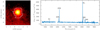 |
Fig. A.1. Background galaxy (BgGx1) detected to the north and its flux-calibrated spectrum. The most prominent features are marked. |
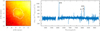 |
Fig. A.2. Background galaxy (BgGx2) detected to the southwest and its flux-calibrated spectrum. The most prominent features are marked. |
All Tables
All Figures
|
Fig. 1. Haro 14 as seen in broadband by MUSE. The FoV is ∼3.8 × 3.8 kpc2 and north is up and east to the left in all the maps presented in this paper. Top-left: image obtained by integrating over the whole observed spectral range. The blue bar corresponds to 1 kpc at the distance of Haro 14. The central square marks the FoV of our previous VIMOS observations. Top-right: “Pure continuum” image in the wavelength range 5400–5600 Å with contours over-plotted. The center of the outermost isophotes lies roughly around the position ΔRA ≃ +5″, ΔDec ≃ +2″. Lower-right: saturated pure continuum image to better visualize the dimmer external parts of the galaxy. Lower-left: synthetic image in the filter R. The color bar shows the calibrated surface brightness in units of mag arcsec−2, the ticks mark the position of two background emission galaxies (see Appendix) and the blue line roughly outlines the bluish regions of the galaxy at intermediate intensity levels (see Sect. 3.3). There are no foreground stars in the observed FoV. |
| In the text | |
|
Fig. 2. Color spatial pattern in Haro 14. Left: (V − I) color index map; bluer colors indicate the bluer (younger) SF regions and red corresponds to the redder (older) stars in the galaxy. The map is not corrected for the contribution of emission lines. Right: increment in the (V − I) color index due to the contribution of emission lines. The blue line roughly delineates the bluish but not ionizing stellar component unveiled in the color map and the black contour corresponds to ΔL(V − I) = 0.01. |
| In the text | |
|
Fig. 3. Surface brightness profiles of Haro 14 built on the synthetic V, R, and I images from MUSE. |
| In the text | |
|
Fig. 4. Haro 14 maps in emission lines: Top-left: Hα emission line flux map of Haro 14; the chain-like structure and the curvilinear feature in the central regions are indicated with white lines. The blue line (bottom-left) corresponds to 1 kpc. Top-right: Hα emission line flux map with the intensity in the inner galaxy regions saturated in order to enhance the faint surface brightness features in the outer galaxy parts; the white lines indicate the most prominent shells and filaments in the galaxy periphery. Bottom-left: Hα equivalent width map (in Å); the blue line roughly delineates the bluish regions of the galaxy at intermediate intensity levels. Bottom-right: [O III] λ5007 flux map. Flux units in the emission line maps are 10−20 erg s−1 cm−2 (per spaxel); the central white cross marks the position of the galaxy peak in continuum. |
| In the text | |
|
Fig. 5. Clumps detected in Haro 14. Top-left: the 29 sources (clumps) detected in continuum (see also Table 3) overplotted on the blue (5400–5600 Å) continuum map. There is an evident clustering of the clumps at the galaxy eastern regions. Top-right: zoom into the central 20″ × 20″. The flux units are arbitrary. Bottom-left: the 55 clumps detected in emission lines (see also Table 4) overplotted on the Hα map; sources detected in Hα and [O III] λ5007 appear in blue, sources detected only in Hα in cyan, and those detected only in [O III] λ5007 in green. Bottom-right: zoom into the central galaxy regions. The intensity scale is logarithmic and the cross marks the position of the continuum peak. |
| In the text | |
|
Fig. 6. MV vs. (V − I) color–magnitude diagram for the sources identified in the continuum maps of Haro 14. |
| In the text | |
|
Fig. A.1. Background galaxy (BgGx1) detected to the north and its flux-calibrated spectrum. The most prominent features are marked. |
| In the text | |
|
Fig. A.2. Background galaxy (BgGx2) detected to the southwest and its flux-calibrated spectrum. The most prominent features are marked. |
| In the text | |
Current usage metrics show cumulative count of Article Views (full-text article views including HTML views, PDF and ePub downloads, according to the available data) and Abstracts Views on Vision4Press platform.
Data correspond to usage on the plateform after 2015. The current usage metrics is available 48-96 hours after online publication and is updated daily on week days.
Initial download of the metrics may take a while.