| Issue |
A&A
Volume 653, September 2021
|
|
|---|---|---|
| Article Number | A124 | |
| Number of page(s) | 6 | |
| Section | Planets and planetary systems | |
| DOI | https://doi.org/10.1051/0004-6361/202141519 | |
| Published online | 21 September 2021 | |
Elimination of a virtual impactor of 2006 QV89 via deep non-detection
1
ESO,
Karl-Schwarzschild-Straße 2,
85748
Garching-bei-München,
Germany
e-mail: This email address is being protected from spambots. You need JavaScript enabled to view it.
2
ESA NEO Coordination Centre,
Largo Galileo Galilei, 1,
00044
Frascati (RM), Italy
e-mail: This email address is being protected from spambots. You need JavaScript enabled to view it.
Received:
11
June
2021
Accepted:
4
August
2021
Abstract
Context. As a consequence of the large (and growing) number of near-Earth objects discovered, some are lost before their orbits can be firmly established and long-term recovery ensured. A fraction of these objects present non-negligible chances of impact with the Earth. We present a method of targeted observations that allow us to eliminate that risk by obtaining deep images of the area where the object would be, should it be on a collision orbit.
Aims. 2006 QV89 was one of these objects, with a chance of impact with the Earth on 2019 September 9. Its position uncertainty (of the order of 1°) and faintness (below V ~ 24) made it a difficult candidate for a traditional direct recovery. However, the position of the virtual impactors could be determined with excellent accuracy.
Methods. In July 2019 the virtual impactors of 2006 QV89 were particularly well placed within a very small uncertainty region, and with an expected magnitude of V < 26. The area was imaged using the ESO Very Large Telescope in the context of the ESA/ESO collaboration on near-Earth objects, resulting in a strongly constrained non-detection.
Results. We eliminated the virtual impactor, even without effectively recovering 2006 QV89, indicating that it did not represent a threat.
Conclusions. This method of deep non-detection of virtual impactors demonstrated a large potential to eliminate the threat of otherwise difficult-to-recover near-Earth objects.
Key words: methods: data analysis / methods: observational / astrometry / minor planets, asteroids: individual: 2006 QV89 / ephemerides / minor planets, asteroids: general
© ESO 2021
1 Introduction
Every year about 2000 new near-Earth objects (NEOs) are discovered, most of them by dedicated surveys1. As soon as the discovery is confirmed, usually after a few days, the objects obtain formal provisional designations and their orbits can be constrained. Together with the orbital calculations it is possible to investigate whether any of these objects also presents a direct threat to our planet by finding possible orbits that are compatible with both the available observational data and correspond to an impact in the future.
On average, for about 96% of the objects, all impact possibilities are quickly excluded. For the remaining 4%, however, scenarios corresponding to a possible future impact remain. In these cases the easiest way to clarify the situation is to perform additional follow-up observations and repeat the computations to check whether future impacts are still compatible with the new data.
This iterative process should ideally continue until all possibilities of impact are excluded or confirmed. However, other factors come into play, especially related to the observability of the targets. Near-Earth objects are typically discovered when close to the Earth, and therefore often quickly recede from our planet, becoming fainter. To extend the observed arc as much as possible, larger telescopes can be used. This is the goal of the collaboration between the European Southern Observatory (ESO) and the European Space Agency (ESA) Planetary Defence Office (Hainaut et al. 2014), in which an 8.2 m unit from the ESO Very Large Telescope (VLT) is used to measure NEOs down to magnitude ~27 or fainter (e.g. 2021 GN2 at G ~ 27.72). Eventually, however, the objects move out of reach of all telescopes. When this happens, no new data can be acquired, often for a very long time, until the object approaches the Earth again and can be recovered.
There are, however, some circumstances when no additional opportunities for observations exist, and therefore the possible threat cannot be excluded. The most likely cause is that an insufficient number of observations could be collected around and immediately after the time of discovery, and therefore our knowledge of the orbit of the object is not sufficient to meaningfully predict its position on the plane of the sky next time it comes close enough to be observed. In this case the object is effectively lost, and no additional observations can be obtained unless it is rediscovered by chance and subsequently linked to the original detections.
For a threatening object, especially one with a high probability of impacts in the future, this situation is unacceptable. Fortunately,an additional approach to clarify the impact threat exists, even without effectively reobserving the lost object. The method, first proposed by Milani et al. (2000), is based on the idea that to exclude a possible impact it is only necessary to ensure that the asteroid is not located on the specific orbit (or family of similar orbits) that will lead it to collide with the Earth. It is usually possible to determine these trajectories very accurately since they are ‘anchored’ by the strong constraint that they have to impact the Earth at a specific future time. It is therefore possible to exclude (or possibly confirm) the impact by just observing the position on the sky where the object would appear if it were on the impacting orbit. A solid non-detection of the object in that area would prove that the impact will not happen, even without detecting the object itself. This technique was considered in the past, for example by Micheli et al. (2019), who excluded an impact by analysing existing archival data containing the location of a possible impacting trajectory. In this paper we present a dedicated observation targeting a specific high-risk object. The method outlined here forms the foundation for a proposed protocol to design, execute, and report such non-detections in a rigorous way that can be properly taken into account by impact monitoring efforts.
Keplerian orbital elements of 2006 QV89 at the epoch MJD = 53978.0.
2 The target
The target is NEO 2006 QV89. It was discovered on 2006 August 29 by the Catalina Sky Survey in Arizona, USA. Various facilities subsequently followed it up until 2006 September 8. The limited observational coverage resulted in a poorly determined orbit. The orbit nevertheless revealed a close approach with the Earth, including a possible impact, on 2019 September 9.
2.1 Orbit determination process
The orbit determination process on which this analysis is based was performed at the ESA NEO Coordination Centre, by using the AstOD software3. The resulting Keplerian orbital elements and their 1σ variation are shown in Table 1. The dynamical model takes into account the  -body gravitational attraction of major Solar System objects (the Sun, the eight planets, the Moon, the 16 most massive asteroids, and Pluto), the parametrised post-Newtonian relativistic contributions and the oblateness of the Sun and the Earth. For the orbit determination process, the weighting scheme described in Veres et al. (2017) was adopted, and the outlier rejection procedure as described in Milani & Gronchi (2010) was applied to the overall dataset. In the case of 2006 QV89, the outlier rejection procedure discarded three observations, and the normalised astrometric root mean square (RMS) residual after the differential corrections process was ~ 0.58. The computed orbit resulting from the differential corrections, and its covariance matrix, formed the input for the skyprint analysis discussed in the next section.
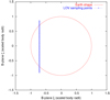 |
Fig. 1 Intersection of the LoV with the cross-section of the Earth in the B-plane of the 2019 September encounter. |
2.2 Position of the virtual impactors
Asteroid impact monitoring methods include several possible approaches, for example the line of variations (LoV) approach (Milani et al. 2005) and Monte Carlo methods. The planned observations of 2006 QV89 required the determination of the family of virtual asteroids that could impact the Earth, being at the same time compatible with the available observations and uncertainties. These are typically referred to as virtual impactors (VIs); the set of VIs that showed an impact with Earth on 2019 September 9 were mapped to a given interval in the line of variations.
Starting from the computed orbit solution (Sect. 2.1), the mapping of the 2019 VIs in the LoV was performed in January of that year using the NIRAT software (Cano et al. 2013). The sampling of the LoV mapped to the impact plane (as defined by Valsecchi et al. 2003) in 2019 September is provided in Fig. 1. Those sampled solutions allowed us to determine the initial state vector of the asteroids that were at the impact limits with the Earth, and thus enabled at a later stage the computation of observational ephemerides any time before the impact chance in 2019 September.
Even if the second largest eigenvalue of the orbit determination covariance was very small compared to the largest one, we performed an additional 2D elliptical sampling of the covariance. This allowed us to obtain a 3σ 2D boundary on the same impact plane. However, negligible changes could be observed in the resulting limiting impact points, as expected by the large difference in the values of the two first eigenvalues. Consequently, we simply used the initial linear sampling of the LoV for all further computations.
2.3 Brightness of the virtual impactors
Based on the (notoriously inaccurate) photometric measurements reported at the Minor Planet Center (MPC), the absolute magnitude of 2006 QV89 is H = 25.5. Modern, well-calibrated sky surveys have accurate photometry, so the quality of the MPC magnitude is bound to improve. The slightly different geometry for the various orbits of the VIs (hence slightly different conversion from observed magnitude to H) does not have an impact on that value.
Small NEOs are significantly elongated, resulting in large light curve amplitudes. Kwiatkowski et al. (2010) reported the amplitude of 12 such objects, with an average light curve range of 1.4 mag, the largest range being 2.2 mag. The extreme, probably pathological case of 1I/‘Oumuamua had a light curve range of 2.5 mag (Meech et al. 2017). The photometric measurements of NEOs provided with the astrometric reports are also likely to be biased towards the brighter part of the light curve because they correspond to times when the object was easier, and therefore more likely to be detected and measured. Overall, the object has therefore the potential to be significantly fainter than predicted from its published H.
Correcting the absolute magnitude for the helio- and geocentric distances and for the solar phase effect (using a customary 0.03 mag deg−1 correction), we would expect V ~ 23.7 at the time our observations were going to be scheduled. Accounting for the possible rotational variability and the uncertainty on H, we set the target magnitude to V = 26 (i.e. over two magnitudes fainter than expected), guaranteeing that the object is brighter than that limit. Coincidentally, this limit also corresponds to an object with a diameter of ~ 10 m, which would cause little or no harm in case of impact.
Geometry and circumstances of the observations of 2006 QV89.
3 Observations
The 2006 QV89 VI was observed with Unit Telescope 1 of the ESO VLT on Paranal, Chile, using the FOcal Reducer and low dispersion Spectrograph 2 (Appenzeller et al. 1998, FORS2), without any filter in order to reach the deepest possible limiting magnitude. The instrument was equipped with its red CCD, a mosaic of two MIT/LL detectors. Only the main chip, A, or CCID20-14-5-3, was used. Its effective field of view covers 7′ × 4′, with 0.252″ binned pixels.
The observations took place in Service Mode on 2019 July 4 and 5; the circumstances and geometry of the observations are listed in Table 2. The data are publicly available from the ESO Science Archive, querying it4 for Observation Blocks numbers (OB ID) 2 445 555 and 2 445 558.
4 Data processing
A bias template was obtained by averaging 14 zero-second exposures with outlier rejection; this template was subtracted from all frames. The level of the sky background on the 2006 QV89 frames was high, about 7500–8800 adu. These images were normalised to a unit background by measuring the median sky level over the central region of the frame, where 2006 QV89 was expected. The background objects were masked. The frames were averaged with outlier rejection, resulting in a template flat-field. As the observationswere obtained offsetting the telescope between each exposure following a random pattern that ensured that each image was pointed at least 2″ from any other image in the sequence, and because the field had only a low density of field stars, the resulting flat-field is extremely clean. Thanks to the 90 images included in this template, the S/N of the flat-field template was over 800. The original 2006 QV89 frames were then divided by the flat-field template and normalised to 1s exposure time. The resulting images were sky-subtracted using SExtractor (Bertin & Arnouts 1996), then aligned on the first frame of the sequence using a dozen field stars. For both nights a background template was created by averaging the image from that night. These images, displayed in Fig. 2, were used as astrometric reference. They were calibrated using over 20 stars from the Gaia DR2 catalogue (Gaia Collaboration 2016, 2018) using 2D second-degree polynomials. The RMS residual on the stars was better than 0.03″. The expected pixel position of each of the 2006 QV89 VIs in each image was computed using their ephemerides from Sect. 2.2 and the astrometric calibration. Figure 2 shows these position in the context of the field objects and Fig. 3 displays traditional stacks of the images aligned on the expected position of the object with the stars trailed.
We used various methods to photometrically calibrate the frames. First, the Gaia stars present in the frames were measured. From the few non-saturated stars, we estimated a zero point (ZP) of 28.8. Second, we used the sky brightness. From the Paranal sky measurements in B, V, R, and I5 we estimated a sky brightness in filter-less observations of 19.7. From the sky brightness in individual frames we measured a ZP = 28.8. Alternatively, we measured the noise of the sky background. As that noise is dominated by the Poisson noise we converted it into a brightness, which results in ZP = 28.7. Third, we considered that the filter-less observations are similar to using the union of the B, V, R, and I filters, and combined the standard ZPs obtained from quality control into ZP = 28.5. The width of the B + V + R+I filters underestimate the width of the CCD passband and the transmission of the individual filters is less than 100%, explaining why this ZP is lower than the other estimates. Overall, we keep ZP = 28.7, with an uncertainty of ~ 0.1 mag.
We subtracted the background templates from the individual frames, resulting in images where the background objects were removed. Because of seeing variations and of the apparent rotation of diffraction patterns caused by the secondary mirror spider, this subtraction is far from perfect, in particular close to the core of each star. Nevertheless, the wider wings of the point spread function and the extended objects are very well subtracted. As the star templates are composed of 44 or 45 images, their noise level is over 6 times better than that of the individual images; this subtraction, therefore, does not significantly degrade the S/N of the images. In addition, as 2006 QV89 moves from frame to frame, and because the star templates were obtained rejecting outliers, the (potential) signal from 2006 QV89 is not affected. We co-added both the original frames and the background-subtracted frames (using either plain average or an average with outlier rejection), resulting in the traditional image showing trailed stars, and a clean image that would show only the moving object. This method has been used, for instance, to detect comet 1P/Halley at magnitude 28.2 (Hainaut et al. 2004). The resulting images are shown in Fig. 4. As a test, artificial objects covering a range of magnitudes were included in the frames; they appear as point sources at the top of the field.
We also produced additional image stacks using various subsets of the images (first and second half of the series, odd and even images). We carefully explored visually the region where the VI was expected, by blinking the various stacks. Faint candidates were investigated and found to be caused by star residuals. We could not identify any convincing candidate; the object is not detected.
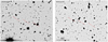 |
Fig. 2 Stack of the images aligned on the stars. The tracks for three VIs from the continuous swarm illustrated in Fig. 1 are indicated. They represent the eastern- and westernmost VIs and the centre of the swarm. Theeastern and western tracks bound the region to be searched. The negative linear grey scale ranges from 2σ below to 15σ above the background. |
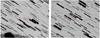 |
Fig. 3 Stack of images aligned on the expected position of the centre VI. The position of the eastern- and westernmost VIs are also indicated. 2006 QV89 appearing between these two extremes would be on a collision orbit. The grey scale is the same as in Fig. 2. |
5 Quantifying the non-detection of 2006 QV89
In order to quantify this non-detection, the maps of limiting magnitudes of the stacks were computed as follows. First, the residual background (at the 0.1 adu level) was subtracted using SExtractor, ensuring that the local mean background is zero. The local noise of the image,
 (1)
(1)
was then estimated by filtering the squared background-subtracted image with a box 5 pixels wide (about
1″). The value of a pixel is
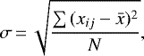
 (2)
(2)
where xij the flux of pixel ij in the background-subtracted image, and N = 25 is the number of pixels in the filter box. By construction, the average value of xij in the box is 0.
This σ is then converted in the limiting magnitude for the 5σ detection of a point source in an d = 1″ = 3.97 pixel aperture
 (3)
(3)
where ZP is the photometric ZP. Figure 5 shows the map of limiting magnitude. The brightest 5σ limits for point sources over the region of interest are 26.8 and 26.1 for the two nights.
Similarly, a map of the significance level at which an object of magnitude M would be measured is computed as
 (4)
(4)
We used ZP = 28.7 (from the previous section). Figure 6 shows the map of the expected S/N for an object with M = 26 (Sect. 2.3). The average expected S/N over the region of interest were 11.2 and 7.8 for the two nights. Even considering the minimum value over the region of interest, 7.1 and 5.7, the object would have been easily detected even at the very pessimistic brightness.
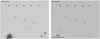 |
Fig. 4 Stack of the background-subtracted frames, aligned on the expected position of the centre VI. The position of the eastern- and westernmost VIs are also indicated. 2006 QV89 appearing between these two extremes would be on a collision orbit. The grey scale is the same as in Fig. 2. Artificial objects were introduced in the images; their magnitudes are indicated. As a reference, 2006 QV89 is expected at mag ~23.7 and must be brighter than 26. |
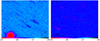 |
Fig. 5 Map of the limiting magnitude of the stacks presented in Fig. 4, at the 5σ level for a point source. |
6 Conclusions
Our study of the threatening NEO 2006 QV89 can be summarized as follows.
- 1.
The orbit of NEO 2006 QV89 was poorly known, but showed chances of collision with the Earth on 2019 September 9. The ephemerides of the virtual impactors were computed.
- 2.
The magnitude of 2006 QV89 expected from the published photometry is V = 23.7. Accounting for the uncertainties on these measurements, and for a possible shape-induced variability, we set V < 26 as the realistic absolute limit beyond which 2006 QV89 cannot realistically exist:
- 3.
We obtained deep observations on two nights with FORS2 on the VLT, on the field where the 2006 QV89 virtual impactors were expected, reaching limiting magnitude 26.8 and 26.5 (5σ for pointsources) on average over the area of interest;
- 4.
The individual images and stack of frames were carefully examined, resulting in constraining the non-detection of the object. At a magnitude of 26, the object would have been detected with a signal-to-noise ratio (S/N) of 11.2 and 7.8 (for each night) on average over the region of interest. The shallowest detections would have been with S/N of 7.1 and 5.7;
- 5.
We can therefore rule out the presence of 2006 QV89 in the VI area; the probability that it is present but not detected is below (1 − P(7.1σ)) ~ 0.000 000 000 256% in the most pessimistic case where its magnitude would be 26, over two magnitudes fainter than expected. As a consequence, even though 2006 QV89 was not recovered, we could be sure that it would not hit the Earth on 2019 September 9.
Given the importance of 2006 QV89 and the attention attracted to the target by this campaign and the possible detectability of the object in 2019 July, a dedicated effort to attempt its actual recovery was carried out by David J. Tholen, using the wide-field MegaCam imager on the Canada-France-Hawaii Telescope (CFHT). Thanks to the wide field of MegaCam, he successfully recovered the object on 2019 July 14, finding it about 3 degrees away from the nominal position, and within 0.1 mag from the expected brightness. His recovery was subsequently confirmed by our team using the Schmidt telescope at Calar Alto, Spain, and published by the Minor Planet Center6.
The observational procedure presented in this work outlines a rigorous process to apply the concepts of Milani et al. (2005) to an actual threatening object. The main goal of this work is that it be used as a reference case for the development of a formal and internationally agreed protocol to eradicate threatening VIs of lost objects via negative observations. This protocol is being developed at the time of preparation of this paper (early 2021). Once completed, it will form the basis on which negative observations can be formally recognised and integrated into the impact monitoring activities carried out by the various international dedicated centres.
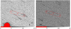 |
Fig. 6 Map of the expected S/N of the VI at its lowest magnitude 26. The regions where this S/Nis below 5 are shaded in red. The zone of interest is indicated by a red contour 10″ around the virtual impactors; the positions of the central VI and the eastern- and westernmost VIs are indicated. |
Acknowledgements
This work is based on observations collected at the European Southern Observatory under ESO programme 5101.C-0575. The authors are grateful to the Paranal staff for their dedication in obtaining our NEO observations for this programme. This work has made use of data from the European Space Agency (ESA) mission Gaia (https://www.cosmos.esa.int/gaia), processed by the Gaia Data Processing and Analysis Consortium (DPAC, https://www.cosmos.esa.int/web/gaia/dpac/consortium). Funding for the DPAC has been provided by national institutions, in particular the institutions participating in the Gaia Multilateral Agreement.
References
- Appenzeller, I., Fricke, K., Fürtig, W., et al. 1998, The Messenger, 94, 1 [NASA ADS] [Google Scholar]
- Bertin, E., & Arnouts, S. 1996, A&AS, 117, 393 [NASA ADS] [CrossRef] [EDP Sciences] [Google Scholar]
- Cano, J. L., Bellei, G., & Martín, J. 2013, in International Astronautical Federation, 6 [Google Scholar]
- Gaia Collaboration (Prusti, T., et al.) 2016, A&A, 595, A1 [NASA ADS] [CrossRef] [EDP Sciences] [Google Scholar]
- Gaia Collaboration (Brown, A. G. A., et al.) 2018, A&A, 616, A1 [NASA ADS] [CrossRef] [EDP Sciences] [Google Scholar]
- Hainaut, O. R., Delsanti, A., Meech, K. J., & West, R. M. 2004, A&A, 417, 1159 [NASA ADS] [CrossRef] [EDP Sciences] [Google Scholar]
- Hainaut, O., Koschny, D., & Micheli, M. 2014, in Asteroids, Comets, Meteors 2014, eds. K. Muinonen, A. Penttilä, M. Granvik, et al. 197 [Google Scholar]
- Kwiatkowski, T., Polinska, M., Loaring, N., et al. 2010, A&A, 511, A49 [NASA ADS] [CrossRef] [EDP Sciences] [Google Scholar]
- Meech, K. J., Weryk, R., Micheli, M., et al. 2017, Nature, 552, 378 [Google Scholar]
- Micheli, M., Cano, J. L., Faggioli, L., et al. 2019, Icarus, 317, 39 [CrossRef] [Google Scholar]
- Milani, A., & Gronchi, G. 2010, Theory of orbits (Cambridge University Press) [Google Scholar]
- Milani, A., Chesley, S. R., Boattini, A., & Valsecchi, G. B. 2000, Icarus, 145, 12 [NASA ADS] [CrossRef] [Google Scholar]
- Milani, A., Chesley, S. R., Sansaturio, M. E., Tommei, G., & Valsecchi, G. B. 2005, Icarus, 173, 362 [NASA ADS] [CrossRef] [Google Scholar]
- Valsecchi, G. B., Milani, A., Gronchi, G. F., & Chesley, S. R. 2003, A&A, 408, 1179 [NASA ADS] [CrossRef] [EDP Sciences] [Google Scholar]
- Veres, P., Farnocchia, D., Chesley, S. R., & Chamberlin, A. B. 2017, Icarus, 296, 139 [NASA ADS] [CrossRef] [Google Scholar]
MPEC 2021-K33: https://www.minorplanetcenter.net/mpec/K21/K21K33.html
AstOD was developed within the NEO Segment of ESA’s Space Situational Awareness Programme.
MPEC 2019-P85: https://www.minorplanetcenter.net/mpec/K19/K19P85.html
All Tables
All Figures
|
Fig. 1 Intersection of the LoV with the cross-section of the Earth in the B-plane of the 2019 September encounter. |
| In the text | |
|
Fig. 2 Stack of the images aligned on the stars. The tracks for three VIs from the continuous swarm illustrated in Fig. 1 are indicated. They represent the eastern- and westernmost VIs and the centre of the swarm. Theeastern and western tracks bound the region to be searched. The negative linear grey scale ranges from 2σ below to 15σ above the background. |
| In the text | |
|
Fig. 3 Stack of images aligned on the expected position of the centre VI. The position of the eastern- and westernmost VIs are also indicated. 2006 QV89 appearing between these two extremes would be on a collision orbit. The grey scale is the same as in Fig. 2. |
| In the text | |
|
Fig. 4 Stack of the background-subtracted frames, aligned on the expected position of the centre VI. The position of the eastern- and westernmost VIs are also indicated. 2006 QV89 appearing between these two extremes would be on a collision orbit. The grey scale is the same as in Fig. 2. Artificial objects were introduced in the images; their magnitudes are indicated. As a reference, 2006 QV89 is expected at mag ~23.7 and must be brighter than 26. |
| In the text | |
|
Fig. 5 Map of the limiting magnitude of the stacks presented in Fig. 4, at the 5σ level for a point source. |
| In the text | |
|
Fig. 6 Map of the expected S/N of the VI at its lowest magnitude 26. The regions where this S/Nis below 5 are shaded in red. The zone of interest is indicated by a red contour 10″ around the virtual impactors; the positions of the central VI and the eastern- and westernmost VIs are indicated. |
| In the text | |
Current usage metrics show cumulative count of Article Views (full-text article views including HTML views, PDF and ePub downloads, according to the available data) and Abstracts Views on Vision4Press platform.
Data correspond to usage on the plateform after 2015. The current usage metrics is available 48-96 hours after online publication and is updated daily on week days.
Initial download of the metrics may take a while.