| Issue |
A&A
Volume 653, September 2021
|
|
|---|---|---|
| Article Number | A91 | |
| Number of page(s) | 11 | |
| Section | The Sun and the Heliosphere | |
| DOI | https://doi.org/10.1051/0004-6361/202141447 | |
| Published online | 14 September 2021 | |
Ti I lines at 2.2 μm as probes of the cooler regions of sunspots
1
Max-Planck-Institut für Sonnensystemforschung, Justus-von-Liebig-Weg 3, 37077 Göttingen, Germany
e-mail: smitha@mps.mpg.de
2
School of Space Research, Kyung Hee University, Yongin, Gyeonggi 446-701, Republic of Korea
3
Lockheed Martin Solar and Astrophysics Laboratory, 3251 Hanover Street, Bldg. 252, Palo Alto, CA 94304, USA
4
Bay Area Environmental Research Institute, NASA Research Park, Moffett Field, CA 94035, USA
Received:
1
June
2021
Accepted:
2
July
2021
Context. The sunspot umbra harbours the coolest plasma on the solar surface due to the presence of strong magnetic fields. The atomic lines that are routinely used to observe the photosphere have weak signals in the umbra and are often swamped by molecular lines. This makes it harder to infer the properties of the umbra, especially in the darkest regions.
Aims. The lines of the Ti I multiplet at 2.2 μm are formed mainly at temperatures ≤4500 K and are not known to be affected by molecular blends in sunspots. Since the first systematic observations in the 1990s, these lines have been seldom observed due to the instrumental challenges involved at these longer wavelengths. We revisit these lines and investigate their formation in different solar features.
Methods. We synthesized the Ti I multiplet using a snapshot from 3D magnetohydrodynamic (MHD) simulations of a sunspot and explored the properties of two of its lines in comparison with two commonly used iron lines, at 6302.5 Å and 1.5648 μm.
Results. We find that the Ti I lines have stronger signals than the Fe I lines in both intensity and polarization in the sunspot umbra and in penumbral spines. They have little to no signal in the penumbral filaments and the quiet Sun, at μ = 1. Their strong and well-split profiles in the dark umbra are less affected by stray light. Consequently, inside the sunspot, it is easier to invert these lines and to infer the atmospheric properties as compared to the iron lines.
Conclusions. The Cryo-NIRSP instrument at the DKIST will provide the first-ever high-resolution observations in this wavelength range. In this preparatory study, we demonstrate the unique temperature and magnetic sensitivities of the Ti multiplet by probing the Sun’s coolest regions, which are not favourable for the formation of other commonly used spectral lines. We thus expect such observations to advance our understanding of sunspot properties.
Key words: line: profiles / line: formation / sunspots / Sun: magnetic fields / starspots / infrared: stars
© H. N. Smitha et al. 2021
 Open Access article, published by EDP Sciences, under the terms of the Creative Commons Attribution License (https://creativecommons.org/licenses/by/4.0), which permits unrestricted use, distribution, and reproduction in any medium, provided the original work is properly cited.
Open Access funding provided by Max Planck Society.
1. Introduction
A regular sunspot mainly consists of a dark umbra surrounded by penumbra as part of its filamentary structure. The umbra can further host relatively brighter features, such as umbral dots, and in some cases, light bridges. Each penumbral filament is made of a bright filament head that is located closer to the umbra and a tail that is the radially outward end of the filament. The darker regions in between the bright filaments are called spines (Lites et al. 1993). For an overview on sunspot formation, structure, and properties, see Solanki (2003), Borrero & Ichimoto (2011), Hinode Review Team (2019).
The umbra is the darkest and the coolest part of a sunspot, and has the strongest magnetic field. Routinely used photospheric spectral lines such as Fe I 6301.5 Å, 6302.5 Å, and 6173 Å in the visible or the Fe I 1.5648 μm and 1.5652 μm lines in the infrared have very weak intensity signals in the umbra. In addition, the low temperatures in the umbra offer ideal conditions for the formation of molecular lines resulting in the heavy blending of the atomic lines in the visible and infrared (see Fig. 5 of Solanki et al. 1992a, for the blending of the Fe I 1.5648 μm line). This makes the inference of atmospheric properties from these atomic lines by means of inversions of the Stokes profiles quite challenging despite their strong polarization signals. Both these issues can be addressed using the Ti lines at 2.2 μm. The lines in this multiplet have low excitation potential, low ionization potential and thus high temperature sensitivity. They are formed mostly in regions with temperatures below 4500 K (Rüedi et al. 1998), such as the sunspot umbra, with weak to no signal in the penumbra or the quiet Sun. Some of the lines in the multiplet are unblended or mainly blended with telluric lines that can be easily removed (Rüedi et al. 1998). These characteristics make the Ti lines at 2.2 μm ideal for isolated umbral observations with little contamination from the penumbra or the quiet Sun.
The Ti I multiplet at 2.2 μm was first observed in a sunspot umbra for an infrared atlas by Hall (1973) at the Kitt Peak National Observatory and later for the atlas by Wallace & Livingston (1992). Their diagnostic potential was first noted by Saar & Linsky (1985), who used them to make the first-ever detection of a magnetic field on an M dwarf, which also happened to be the strongest field discovered up to that point on a cool star (Saar 1994). Later, Saar et al. (1987) used the Ti multiplet to study late K and M dwarfs. Recently, the Ti lines were observed by Kochukhov et al. (2009) to measure magnetic fields on M dwarfs using the cryogenic high-resolution cross-dispersed infrared echelle spectrograph (CRIRES, Kaeufl et al. 2004) on the Very Large Telescope (VLT) of the European Southern Observatory. For a historical context on how these lines shaped our understanding of the stellar magnetic fields, see Saar (1994, 1996).
In the context of solar magnetic field measurements, the potential of the Ti lines was first noted by Rüedi et al. (1995). Later, Rüedi et al. (1998) presented the first systematic scans of the sunspot umbra observed using the Ti I 2.2 μm lines. Using these observations, the authors found that the sunspots are made of two distinct cool components: one component with strong vertical magnetic field associated with the umbra and another weakly inclined magnetic component in the penumbra. These same observations were later used by Rüedi et al. (1999) to study the Evershed flow in the cooler channels of the penumbra. Observations in the Ti I line at 2.231 μm were used by Penn et al. (2003a,b) to measure the velocities of the Evershed outflow, as well as umbral and penumbral magnetic fields. The same line will also be observed by LOCNES: low-cost NIR extended solar telescope to study the effects of cooler plasma on the disk-integrated flux and mean magnetic field on the Sun in order to understand the stellar jitter in radial velocity technique arising due to activity on other stars (Claudi et al. 2018). The radial velocity technique is used for extrasolar planet detection.
The high temperature sensitivity and high magnetic sensitivity of the Ti I lines form a unique combination for probing the sunspot umbra. Their Zeeman sensitivity is greater than the visible lines, such as the commonly used Fe I 6300 Å pair observed by Hinode/SOT-SP (Ichimoto et al. 2008). As discussed in Rüedi et al. (1998), the Ti I lines are less affected by molecular blends and stray light from the surrounding penumbra and quiet Sun regions. Other than the McMath–Pierce Telescope at the National Solar Observatory at Kitt Peak, no other telescopes have been used to observe these interesting lines on the Sun, partly due to the lack of instruments that can observe at these wavelengths. However, the Cryo-NIRSP instrument (Fehlmann et al. 2016), available at the newly constructed DKIST (Elmore et al. 2014; Rimmele et al. 2020), will be able to observe the Ti lines at 2.2 μm for the first time at a high spatial and spectral resolution.
In the present paper, we investigate the diagnostic potential of Ti I line around 2.2 μm. To this end, we synthesized the Ti multiplet from a sunspot simulation of Rempel (2012), along with two commonly used iron lines in the visible and infrared. We then carried out a comparative study to explore the unique potential of the Ti lines and how they can be used to study different features of a Sunspot.
2. Ti I multiplet at 2.2 μm
The titanium multiplet of interest has six lines (Blackwell-Whitehead et al. 2006; Saloman 2012), five of which were discussed in Rüedi et al. (1998). The atomic details of all the lines taken from the Vienna Atomic Line Database (VALD) are presented in Table 1. We have also included the two commonly observed iron lines at 6302 Å and 15 648 Å in the table.
Atomic details of the Ti I multiplet at 2.2 μm and two other iron lines (bottom two rows) often used for sunspot diagnostics.
The Zeeman splitting of a spectral line increases as λ2geff, where λ is the central wavelength and geff is the effective Landé factor. Since the Doppler width of the line increases linearly with λ, the observable magnetic splitting of the spectral line is, therefore, ∝λgeff. For the titanium multiplet and the two iron lines, λgeff are indicated in the last column of Table 1. In the titanium multiplet, the 22 310 Å line has the largest magnetic sensitivity which is 3.5 times larger than the Fe I 6302 Å line and nearly 1.2 times the sensitivity of the Fe I 1.56 μm line. From the Zeeman splitting patterns shown in Rüedi et al. (1998), the Ti I 22 310 Å is the only line in this multiplet with a normal Zeeman triplet. However, it is weaker than the other lines due to its smaller line strength (log(gf)).
From the low-resolution observations presented in Rüedi et al. (1995), four lines in the titanium multiplet at 22 211 Å, 22 232 Å, 22 274 Å, and 22 310 Å have no known blends of solar origin. Among these, the most magnetically sensitive line at 22 310 Å with geff = 2.5 has a strong telluric blend, which can be easily removed using the procedure described by the above authors and originally proposed by Hall (1973), cf. Saar & Linsky (1985). Another interesting line in the multiplet is the one 22 211 Å, with the second largest Landé factor geff = 2.0. This line is again blended by telluric lines but they too are easily removable (Rüedi et al. 1995). The only line (that we know of) with a blend of solar origin is the one at 21 897 Å, which has a comparatively small geff. Recently, high-resolution observations of the Ti I 22 274 Å line in M dwarfs using CRIRES by Kochukhov et al. (2009) revealed that it is unblended in stars hotter than M2. On the Sun, high-resolution observations from DKIST will be able to provide more insights into the presence of blends close to the Ti lines.
For further analysis in the rest of the paper, we consider the profiles of only two lines in the titanium multiplet with extreme properties: the line with largest magnetic sensitivity and smallest log(gf) at 22 310 Å, and the one with largest line strength but small Landé factor (geff = 1.17) at 21 897 Å.
3. Spectral profiles
3.1. Synthesis
To investigate the formation of titanium lines in a sunspot and the quiet Sun, we used a three-dimensional magnetohydrodynamic (MHD) simulation (Rempel 2012, 2015) generated using the MURaM code (Vögler et al. 2005). The simulation box extends to (61.44 × 61.44 × 2.97) Mm in the x, y, z directions, respectively, with a grid spacing of 48 km in the xy-direction and 24 km in the vertical direction. However, we only use a piece of the full cube for spectral synthesis. The maps of temperature, magnetic field strength, and magnetic field inclination from this MHD cube at log(τ) = 0.0, −0.8 and −2.3 are shown in Fig. 1. We refer to log(τ5000) simply as log(τ).
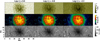 |
Fig. 1. Maps of temperature (first row), magnetic field strength (second row), and magnetic field inclination (third row) from the MHD sunspot simulation at log(τ) = 0.0, −0.8, and −2.3. |
The Stokes profiles (I, Q, U, V) were synthesized in local thermodynamic equilibrium (LTE) by solving the 1D radiative transfer equation along each column of the MHD cube, a scheme known as 1.5D LTE, using the SPINOR code Solanki (1987), Frutiger et al. (2000) at μ = 1.0, that is, all computations correspond to solar disc centre. As previously mentioned, we discuss the synthetic Stokes profiles of only two lines from the Ti multiplet at 21 897 Å and 22 310 Å and compare them with the profiles of Fe I 6302.5 Å and 15 648 Å.
3.2. Height of formation
To determine the atmospheric layers sampled by the titanium lines, we compute their ‘height of formation’ in the same way as in Smitha & Solanki (2017). The height of formation of a given line is assumed to be the centroid of the range of heights sampled by the intensity profiles weighted by their response functions (Beckers & Milkey 1975). Here, we used the intensity response to perturbations in temperature. The maps of the height of formation so obtained are shown in Fig. 2. The heights are indicated with respect to a reference z = 0 km geometrical layer which corresponds to log(τ) = 0, averaged over the simulation box. The Ti I 22 310 Å line is formed at similar heights as the 21 897 Å line and, hence, we only discuss the latter in detail.
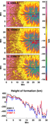 |
Fig. 2. Maps of height of formation of the three lines λ = 6302.5 Å (panel a), 15 648.5 Å (panel b), and 21 897.4 Å (panel c). The height of formation is the centroid of the intensity response function to temperature. Bottom panel: we have plotted the heights of formation along the horizontal black lines, averaging in the y-direction over the narrow region between the two black lines covering four pixels. |
The heights of formation of the three lines at Fe I 6302 Å, Fe I 15 648 Å, and the Ti I 21 897 Å averaged over four pixels in the y-direction covering different features in the cube are shown in the bottom panel. The fall in the formation height of the lines from the quiet Sun to the umbra due to the Wilson depression is clearly seen. In the quiet Sun, the formation height of the titanium line falls in between the two iron lines. In the sunspot penumbra and the umbra, the titanium line is formed slightly higher than the Fe lines. The Fe I infrared line at 1.56 μm is formed the lowest everywhere in the simulation domain. These results are in agreement with the heights determined using the contribution functions by Rüedi et al. (1998).
3.3. Stokes profiles in different features
3.3.1. Normalization
The synthetic Stokes profiles computed from the sunspot cube can be normalized in two different ways, one with the spatially averaged quiet Sun intensity (Ic − qs) and the other using the local continuum in that pixel (Ic − loc). In the literature we find both approaches being used depending on the problem that is addressed. In the brighter features such as the granules, the Ic − qs is smaller than Ic − loc and in the dark sunspot umbra, the Ic − loc is only a small fraction of Ic − qs. Thus, the Stokes profiles have different amplitudes depending on the normalization used. Since the normalization with Ic − qs is more commonly used for the inversion of Stokes profiles (Bellot Rubio et al. 2000; Socas-Navarro et al. 2004; Riethmüller et al. 2008a, 2013; Tiwari et al. 2015), we follow the same in the rest of the paper.
3.3.2. Equivalent widths and normalized line depths
In Fig. 3, we compare the equivalent widths (EW; first column), normalized line depths (NLD, the line depth of Stokes I profiles normalized to the average quiet Sun continuum intensity, middle column), and maximum circular polarization (last column). Maps are presented for the Ti I 22 310 Å and 21 897 Å lines along with the two iron lines at 6302 Å and 15 648 Å. In the quiet Sun, both EW and NLD are small for the titanium lines. For the Ti I 22 310 Å line, the NLD is < 0.05 and EW is < 10 mÅ. Due to its slightly larger log(gf), EW reaches 50 mÅ for the Ti I 21 897 Å line along with NLD up to 0.2. In comparison, the two iron lines at 6320 Å and at 1.56 μm have much larger EW and NLD in the quiet Sun. Here, the EW of the Fe I 6302 Å line ranges from 50 mÅ to 150 mÅ, with the NLD ranging from 0.2 − 1.3. The NLD of the Fe I 6302 Å line exceeding 1.0 is commonly obtained from pixels where the local continuum is higher than the spatially averaged quiet Sun continuum. The infrared iron line at 1.56 μm, although it has smaller NLD (< 0.55) compared to the visible line, has larger EW due to its longer wavelength. In the quiet Sun, the EW of the iron 1.56 μm line varies between 50 and 200 mÅ. From the circular polarization maps in Fig. 3, both titanium lines at 21897 Å and 22310 Å have little to no V/Ic − qs signal in the quiet Sun, while the V/Ic − qs of the iron lines reaches values as high as 10%−15% in kilo-gauss magnetic elements.
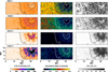 |
Fig. 3. First and second columns: maps of the equivalent widths and normalized line depths of the intensity profiles. Last columns: maps of maximum circular polarization. All quantities are plotted for four lines the Fe I 6302.5 Å and 1.56 μm lines (top panels), and the Ti I 22 310 Å, and 21 897 Å lines (bottom panels). Contours mark the penumbra-umbra and penumbra-quiet sun boundaries. |
In the sunspot umbra, the titanium lines have a clear advantage. The EW of the stronger line at 21 897 Å ranges from 400 mÅ to 1.1 Å and the NLD varies between 0.1 and 0.4. The distribution of EW and NLD over all the pixels peak around 900 mÅ and 0.15, respectively. We note that the larger values are not visible in Fig. 3 as the EW color scale is saturated at 800 mÅ, so that the change in EW of the other lines can be seen as well. The 21 897 Å line undergoes anomalous Zeeman splitting and we see multiple Zeeman components in the Stokes profiles (see Fig. 1 of Rüedi et al. 1998). Given it is a normal Zeeman triplet, the Ti I 22 310 Å line is split into its three Zeeman components. To compute the EW, we integrate over all the Zeeman components for all the lines. The EW and NLD in the umbra range between 100 − 400 mÅ and 0.05 − 0.2, respectively. For both Ti I 21 897 Å and 22 310 Å lines, the EWs measured in Rüedi et al. (1998, see their Figs. 3 and 4) are smaller while the NLD values are larger than in our synthesis. This is because in Rüedi et al. (1998) the EW and NLD were measured in the absence of a magnetic field.
The Fe I 1.56 μm line, due to its large Landé factor geff = 3.0, is fully split in the umbra and penumbra. In the umbra, its EW is comparable to the Ti I 22 310 Å line. The EW of the 1.56 μm line varies between 100 and 300 mÅ with a peak of the distribution around 200 mÅ. Its NLD over the umbra is smaller than the Ti I 22 310 Å line and it varies between 0.02 and 0.2 with a peak of the distribution at 0.05. Of all the four lines presented in Fig. 3, the Fe I 6302 Å has the smallest EW (70 − 250 mÅ) and NLD (0.01 − 0.2).
The circular polarization profiles of the two iron lines at 6302 Å and the 1.56 μm are Zeeman saturated at umbral magnetic fields. The lines in the titanium multiplet including those considered in Fig. 3 (last column) may seem not to suffer from Zeeman saturation, although they are clearly completely split in the umbra. This is due to a combination of low excitation potential, low ionization potential and low abundance (Rüedi et al. 1995) and the anti-correlation between magnetic field strength and temperature in sunspot umbrae (e.g. Martinez Pillet & Vazquez 1990; Kopp & Rabin 1992; Tiwari et al. 2015). In the umbra, the Ti lines at 21 897 Å and 22 310 Å have V/Ic − qs signals exceeding 15% while for the Fe I 6302 Å and 1.56 μm lines, they do not exceed 5%.
In Figs. 4–6, we compare the Stokes profiles, I/Ic − qs, Q/Ic − qs and V/Ic − qs of the two iron lines and the two titanium lines, with pixels representing different features within the simulation. The chosen pixels are indicated on the maps by yellow boxes. We discuss them in more detail in the sections below.
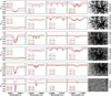 |
Fig. 4. Stokes I profiles from different features of the sunspot and the quiet Sun. From top to bottom: umbral dots, dark umbral core, penumbral filament head, spine in penumbra, penumbral filament tail, and quiet Sun. At each feature, we show profiles from four sample pixels and indicate the equivalent widths (in mÅ) and normalized line depths. These pixels are at the centers of the squares marked on the images in the last column. The profiles are shown for both the Fe I and the Ti I spectral lines. They are normalized to the spatially averaged quiet Sun continuum intensity (Ic − qs). The contrast on the last column was adapted for better representation of the different features. |
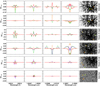 |
Fig. 5. Stokes Q/Ic profiles from different features of the sunspot and the quiet Sun computed at two iron and two titanium lines. Details are the same as in Fig. 4 but for the Q/Ic − qs profiles. |
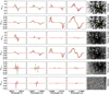 |
Fig. 6. Stokes V/Ic profiles from different features of the sunspot and the quiet Sun computed at two iron and two titanium lines. Details are the same as in Fig. 4 but for V/Ic − qs profiles. |
3.3.3. Umbra
A typical sunspot umbra consists of a dark background and relatively brighter umbral dots. The dark nucleus, namely, the part of the umbra with the darkest background and few umbral dots, which has the strongest magnetic field in the umbra (Kopp & Rabin 1992; Solanki & Montavon 1993), generally covers 10% to 20% of the total umbral area (Solanki 2003). Due to the low temperature of the plasma, the conditions here are ideal for the formation of titanium lines while the iron lines have very weak signals. In the first two columns of Figs. 4–6, we show the intensity and polarization profiles of the two iron lines at 6302 Å and 1.56 μm. These should be compared with the profiles of Ti I 22 310 Å and 21 897 Å (Cols. 3 and 4, respectively). The profiles in the first row of all three figures are from umbral dots, while the second row shows examples from the dark umbral nucleus.
In the pixels from the umbral dots, all the four spectral lines considered in the figures have intensity profiles with NLD greater than 0.1. The Ti I 21 897 Å line has the largest NLD and EW, followed by the Fe I 1.56 μm line (see I/Ic − qs profiles plotted in the top row of Fig. 4). In brighter umbral dots (indicated by purple and orange lines), the NLD and EW of the 6302 Å intensity profiles are comparable to the Fe I 1.56 μm. In the remaining two umbral dots shown in the figure, they are smaller. On average, the Ti I 22 310 Å line has smaller NLD and EW in the four representative pixels from umbral dots chosen here. The Zeeman components of the Fe I 1.56 μm and the two Ti lines are completely split in the umbral dots. All the four lines have comparable amplitudes of both Q/Ic − qs(∼5%−10%) and V/Ic − qs(∼5%) profiles. The two iron lines have been used in several papers to study the properties of umbral dots (see e.g. Socas-Navarro et al. 2004; Riethmüller et al. 2008b; Watanabe et al. 2009, 2012; Yadav et al. 2018). For the reasons previously stated (large EW and NDL combined with strong polarization signals), observations in the Ti multiplet will provide new insights into the umbral dots and their fine-scale structures (Schüssler & Vögler 2006; Bharti et al. 2007).
In the dark umbral nucleus, the Fe I 6302 Å and 1.56 μm lines nearly disappear with NLD much less than 0.1, although their EW > 100 mÅ. In comparison, the Ti lines are stronger. The EW of Ti I 21 897 Å is greater than 800 mÅ and in a few pixels it even exceeds 1 Å. The Zeeman components of the Ti I 22 310 Å line are far apart and they have an EW between 250 and 350 mÅ. Both these Ti lines have NLD between 0.1 and 0.2, which is greater than the iron lines. In polarization, Q/Ic − qs and V/Ic − qs signals in the iron lines are three times smaller in amplitude.
3.3.4. Penumbra
According to the uncombed configuration of the penumbra (Solanki & Montavon 1993; Solanki 2003), the magnetic field in the sunspot penumbra is composed of two components, one is the strong and vertical component known as the spines and the other is the weakly inclined component called the inter-spines or the filaments (Lites et al. 1993). The spines are dark and cooler compared to the filaments (e.g. Tiwari et al. 2013). They offer favourable conditions for the formation of the Ti lines. From Fig. 4, the EW and NLD of the two titanium lines 21 897 Å and 22 310 Å in the penumbral spines are larger than those of the iron lines (fourth row). In the spines, the profiles from Fe I 1.56 μm lines are although fully split and have EW > 180 mÅ, their NLD are less than 0.1. The EW and NLD of the Fe I 6302 Å line in the penumbral spines are comparable to its profiles in the dark umbra. From Figs. 4–6, we can see the two Ti lines have stronger polarization signals than the Fe lines in the dark penumbral spines. In the penumbral filament, however, the Fe lines are much stronger than the Ti lines in both intensity and polarization due to larger plasma temperatures. Tiwari et al. (2015) demonstrated that penumbral filament tails are in general darker and cooler than the filament heads (see also Bharti et al. 2010; Tiwari et al. 2013). From rows 3 and 5 of Figs. 4–6, we see that the titanium lines are weak in the filament head as well as in the filament tail. We do not see a significant strengthening of the signal due to a drop in temperature from the head to the tail. This is because the profiles shown in the figures are selected from the tails of the outer penumbral filaments. Here, the difference in temperature between the filament head and filament tail is only about 300 K, on average (Tiwari et al. 2013). Since the temperature of the tails in the inner penumbra is lower and comparable to the temperature in the spines (Tiwari et al. 2013), it is possible that the Ti line has a stronger signal in the tails of inner penumbral filaments (see Fig. 3). The profiles from the inner penumbral filaments are not shown in Figs. 4–6. Also, the tails and heads of filaments in the simulation are not as localized and distinct as in the observations – and quantitative differences between the observations and simulations do exist.
3.3.5. Quiet Sun
According to Fig. 2, the Ti lines are formed in the upper photosphere. Although the granule temperature drops rapidly with height in the atmosphere, it is not cool enough for the formation of the titanium multiplet. They have nearly no signal in both intensity and polarization in the quiet Sun, with the exception of Ti I 21 897 Å line. Due to its large log(gf), this line has weak measurable signals, although these are not found in the immediate vicinity of the sunspot. In Fig. 3 (second column, bottom row), the 21 897 Å line forms a dark ring around the penumbra, signifying basically no line absorption. This is due to the presence of the magnetic canopy, which, at the height of formation of Ti lines, extends beyond the photospheric (log(τ) = 0.0) penumbral boundary (Giovanelli & Jones 1982; Solanki et al. 1992b, 1994). Above the canopy base, the gas density is considerably reduced as a result of the magnetic pressure, so that the absorption in all lines is considerably reduced there. This forces much of the line to be formed below the canopy, where the temperature is relatively high. While this does not affect the Fe I lines to a large extent, as they are not so sensitive to temperature, the absorption due to the Ti lines is very small due to their strong temperature sensitivity. Altogether, this results in very weak Ti I lines. These signals are sufficiently weak as to not contaminate the sunspot observations through straylight, providing desirable conditions for studying the nature of the cool penumbral spines or the dark umbra. In the sunspot umbra, the Fe lines not only have weak signals but could also suffer contamination from the strong quiet-Sun and penumbral signals.
4. Simulation of observations
4.1. Degradation
The Stokes profiles of the titanium line and the iron lines were degraded to simulate real observations. Out of the five lines in the titanium multiplet, we chose the one at 21 897 Å since it has the largest log(gf) and is very strong in the umbra and penumbral spines, with EWs as high as 800 mÅ (see Fig. 4). This line was degraded according to the specifications of the DKIST Cryo-NIRSP instrument which has a spatial sampling of 0.15″ pix−1 and a spectral resolving power of 100 000 for on-disk observations. The iron line at 6302 Å was degraded to the specifications of Hinode/SOT-SP, which has a similar spatial sampling of 0.16″ pix−1 (normal mode) and a spectral resolution of 21.5 mÅ pix−1. Then a random noise was added by convolving with a Gaussian distribution with standard deviation of 1 × 10⁻³ Ic − qs. The profiles were further degraded with a global 10% stray light in way similar to that described in Milić et al. (2019).
4.2. Inversion of the Stokes profiles
After degradation, the profiles were inverted using the code SPINOR 1D (Frutiger et al. 2000), which is based on the STOPRO routines (Solanki 1987). SPINOR solves the radiative transfer equations for polarized light to retrieve the atmospheric conditions independently at every pixel inside the field of view. We use a simple atmospheric model with three nodes for the temperature, magnetic field vector, and LOS velocity as well as one node for the microturbulent velocity. For the optimum placement of the nodes for the inversion of the Ti I line, we first inverted a narrow stripe covering different features like the quiet Sun, penumbra, and the darkest umbra. In each trial, we slightly shifted the nodes and calculated the mean-χ2 of the narrow stripe. A plot of the mean-χ2 as a function of the node position, gave us a parabola-like curve. The middle and top nodes were chosen based on the location where the curve reaches minimum. In the end, the nodes were placed at log(τ) = 0.0, −0.8, and −2.3 which are also suitable for inverting the Hinode/SOT-SP observations (Castellanos Durán et al. 2020).
Using the single component model described above (i.e. without accounting for stray light in the inversion), we were able to easily invert the Ti I 21 897 Å line. However we were unable to get a good fit to the Fe I 6302 Å line profiles. In order to model the stray light component in the iron line, we performed tests by adding a second component model atmosphere with three nodes for the temperature, along with one each in the LOS velocity and magnetic field strength to account for any net wavelength shift due to the degradation, as well as a filling factor. The two-component model slightly improved the fits to the iron line. Clearly, the iron line is much more affected by stray light compared to the titanium line. In the umbra, the strong linear and circular polarization signals of the titianium line offers an additional advantage during inversions. For observations, the absence of strong solar blends is another strong advantage.
In Fig. 7 (right panels), we compare the fits to both titanium and iron lines using single component atmosphere at two sample pixels in the umbra. In these pixels, the Fe I 6302 Å line displays a weak signal in both intensity and polarization, and is strongly affected by spatial degradation and stray light. Here, the Ti I 21 897 Å line scores better. For testing, we inverted the Stokes profiles both with and without the degradation (Sect. 4.1). Our tests showed that the complexity of finding a good fit to the Fe I line increases substantially after the degradation (especially in the dark regions). On the other hand, the Ti I line did not show such a behaviour. The inversion retrieved good fits to the synthetic profiles in dark regions with and without the degradation.
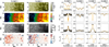 |
Fig. 7. Atmospheric maps from the inversion of iron and titanium lines. Left: maps of the temperature (a, e), magnetic field strength (b, f), inclination (c, g), and LOS velocity (d, h) at log(τ) = − 0.8, obtained by inverting the Ti I 21 897 Å (first column) and Fe I 6302 Å (second column) lines. In the LOS velocity maps, blue indicates upflows and red downflows. Right: fit to the degraded Stokes profiles of the Ti and Fe lines at two sample pixels marked on the temperature maps. |
In the same figure we also show maps of the inverted atmosphere obtained from the titanium and iron lines. We only show the maps at log(τ) = − 0.8 since the middle node is the best constrained. Due to the difference in the height of formation of the two lines (see Fig. 2), the atmospheric maps in the fist and second column of Fig. 7 appear different. In the quiet Sun, the maps derived from the Ti I line appear noisy due to the low signal, clearly seen in the LOS velocity map. The titanium line nevertheless provides results that appear reasonable, with the quality of the fits also good. It’s strong suit is in the umbra and in penumbral spines.
In real observations, heavy blending by molecular lines will further complicate the determination of atmospheric parameters in the dark umbral regions. Sample profiles from the Hinode/SOT-SP observations illustrating the numerous weak lines blending the iron lines around 6302 Å in the umbra are shown in Fig. A.1. The spatially coupled inversions (van Noort 2012; van Noort et al. 2013) might be suitable for fitting a stray light affected profile, but this remains to be tested. On the other hand, the Ti I 21 897 Å line could be inverted using 1D inversion codes. However, the caveat is that the molecular blending of the 6302 Å line only became visible in the very low stray light observations of Hinode. Therefore, it cannot be ruled out that such observations could also reveal the molecular blending of the Ti I lines.
5. Conclusions
In this paper, we explore how useful the lines in the Ti multiplet at 2.2 μm are in probing the different fine-scale features of a sunspot. Due to their low ionization potential and low excitation potential, the Ti lines are highly sensitive to temperature. They are formed only in cooler regions, increasing in strength with decreasing temperature until about 4000 K, but decreasing again below roughly 3500 K due to the formation of TiO molecules (Rüedi et al. 1998). Hence, they are strongest in the sunspot umbra and penumbral dark spines. Due to their longer wavelengths and large Landé factors (mainly the 22 310 Å line), they are strongly magnetically sensitive (λgeff). All the lines in the Ti multiplet have λgeff greater than the commonly used line Fe I 6302 Å. The Ti I 22 310 Å line, with geff = 2.5, is somewhat more magnetically sensitive than the Fe I 1.56 μm, although this might be offset by the fact that it is formed higher in the atmosphere, where the magnetic field is generally slightly weaker. The synthetic observations from an MHD simulation reveal that the Ti lines at 21 897 Å and 22 310 Å (two out of the six lines in the multiplet we chosen for the detailed analysis), have stronger signals (larger EW, larger line depth, and stronger polarization signals) in the dark umbra and penumbral spines, compared to the Fe I 6302 Å and 1.56 μm lines. The Ti I multiplet may also provide unique information about ultra cool parts of the umbra (T < 3800 K at log τ = 0; Fig. A.1), which have mostly remained unexplored.
Tests conducted by degrading the Stokes profiles of the Ti I 21 897 Å and Fe I 6302 Å lines, followed by inversions, have revealed that the Ti line is much less affected by stray light compared to the iron line. The Ti line could be more easily inverted compared to the iron line inside the simulated spot. That is to say that the fit to the Ti lines could be easily obtained even with a simple three-node single component atmosphere. Based on the observations of the Ti multiplet presented in Rüedi et al. (1995, 1998), Penn et al. (2003a), four out of six lines do not have any blend of solar origin. This is particularly advantageous for observing sunspot umbrae since the Fe I 6302 Å and 1.56 μm lines are blended by solar molecular lines.
Since the Ti lines sample only the regions of low temperature, they complement the Fe lines, so that both sets of lines can be used together to probe both cool and hotter structures in a sunspot. For example, the high resolution observations from Hinode and ground-based telescopes have revealed a variety of small-scale structures within the penumbra that exhibit different physical properties. The iron lines and titanium lines together can be used to understand the properties of both cooler and hotter features within the penumbra, such as the interaction between the hot penumbral filaments and the cool spines.
The Evershed flow in the cooler channels of the penumbra measured using the Ti I line by Rüedi et al. (1999) was at a spatial resolution of 2″ − 3″. To date, the Evershed flow has been studied in great detail using the current generation high-resolution data at different spectral ranges. This type of analysis has not been undertaken for the Ti 2.2 μm lines. It will be quite interesting to explore how the DKIST observations will fit into our current understanding of this dynamic phenomenon.
Thanks to a range of magnetic sensitivities and line strengths, the Ti I multiplet at 2.2 μm offers a set of lines to choose from. The high resolution data recorded by the Cryo-NIRSP instrument on DKIST will offer many possibilities of exploiting them.
Acknowledgments
We thank M. Rempel for kindly providing the MHD cube. HNS thanks H. P. Doerr for discussions regarding stray light. This project has received funding from the European Research Council (ERC) under the European Union’s Horizon 2020 research and innovation programme (grant agreement No. 695075). J.S.C.D. was funded by the Deutscher Akademischer Austauschdienst (DAAD) and the International Max Planck Research School (IMPRS) for Solar System Science at the University of Göttingen. S.K.T. gratefully acknowledges support by NASA contract NNM07AA01C (Hinode). Hinode is a Japanese mission developed and launched by ISAS/JAXA, with NAOJ as domestic partner and NASA and STFC (UK) as international partners. It is operated by these agencies in co-operation with ESA and NSC (Norway). This work has made use of the VALD database, operated at Uppsala University, the Institute of Astronomy RAS in Moscow, and the University of Vienna. This research has made use of NASA’s Astrophysics Data System.
References
- Beckers, J. M., & Milkey, R. W. 1975, Sol. Phys., 43, 289 [NASA ADS] [CrossRef] [Google Scholar]
- Bellot Rubio, L. R., Collados, M., Ruiz Cobo, B., & Rodríguez Hidalgo, I. 2000, ApJ, 534, 989 [NASA ADS] [CrossRef] [Google Scholar]
- Bharti, L., Joshi, C., & Jaaffrey, S. N. A. 2007, ApJ, 669, L57 [NASA ADS] [CrossRef] [Google Scholar]
- Bharti, L., Solanki, S. K., & Hirzberger, J. 2010, ApJ, 722, L194 [NASA ADS] [CrossRef] [Google Scholar]
- Blackwell-Whitehead, R. J., Lundberg, H., Nave, G., et al. 2006, MNRAS, 373, 1603 [NASA ADS] [CrossRef] [Google Scholar]
- Borrero, J. M., & Ichimoto, K. 2011, Liv. Rev. Sol. Phys., 8, 4 [Google Scholar]
- Castellanos Durán, J. S., Lagg, A., Solanki, S. K., & van Noort, M. 2020, ApJ, 895, 129 [CrossRef] [Google Scholar]
- Claudi, R., Ghedina, A., Pace, E., et al. 2018, in Ground-based and Airborne Telescopes VII, eds. H. K. Marshall, & J. Spyromilio, SPIE Conf. Ser., 10700, 107004N [Google Scholar]
- Elmore, D. F., Rimmele, T., Casini, R., et al. 2014, in Ground-based and Airborne Instrumentation for Astronomy V, eds. S. K. Ramsay, I. S. McLean, & H. Takami, SPIE Conf. Ser., 9147, 914707 [Google Scholar]
- Fehlmann, A., Giebink, C., Kuhn, J. R., et al. 2016, in Ground-based and Airborne Instrumentation for Astronomy VI, eds. C. J. Evans, L. Simard, & H. Takami, SPIE Conf. Ser., 9908, 99084D [NASA ADS] [Google Scholar]
- Frutiger, C., Solanki, S. K., Fligge, M., & Bruls, J. H. M. J. 2000, A&A, 358, 1109 [NASA ADS] [Google Scholar]
- Giovanelli, R. G., & Jones, H. P. 1982, Sol. Phys., 79, 267 [NASA ADS] [CrossRef] [Google Scholar]
- Hall, D. N. B. 1973, An Atlas of Infrared Spectra of the Solar Photosphere and of Sunspot Umbrae, in the Spectral Intervals 4040 cm-1 -5095 cm-1; 5550 cm-1 -6700 cm-1; 7400 cm-1 -8790 cm-1 (Tucson: Kitt Peak National Observatory) [Google Scholar]
- Hinode Review Team (Al-Janabi, K., et al.) 2019, PASJ, 71, R1 [CrossRef] [Google Scholar]
- Ichimoto, K., Lites, B., Elmore, D., et al. 2008, Sol. Phys., 249, 233 [Google Scholar]
- Kaeufl, H. U., Ballester, P., Biereichel, P., et al. 2004, in Ground-based Instrumentation for Astronomy, eds. A. F. M. Moorwood, & M. Iye, SPIE Conf. Ser., 5492, 1218 [NASA ADS] [CrossRef] [Google Scholar]
- Kochukhov, O., Heiter, U., Piskunov, N., et al. 2009, in 15th Cambridge Workshop on Cool Stars, Stellar Systems, and the Sun, ed. E. Stempels, AIP Conf. Ser., 1094, 124 [Google Scholar]
- Kopp, G., & Rabin, D. 1992, Sol. Phys., 141, 253 [NASA ADS] [CrossRef] [Google Scholar]
- Lites, B. W., Elmore, D. F., Seagraves, P., & Skumanich, A. P. 1993, ApJ, 418, 928 [NASA ADS] [CrossRef] [Google Scholar]
- Martinez Pillet, V., & Vazquez, M. 1990, Ap&SS, 170, 75 [NASA ADS] [CrossRef] [Google Scholar]
- Milić, I., Smitha, H. N., & Lagg, A. 2019, A&A, 630, A133 [CrossRef] [EDP Sciences] [Google Scholar]
- Penn, M. J., Cao, W. D., Walton, S. R., Chapman, G. A., & Livingston, W. 2003a, Sol. Phys., 215, 87 [NASA ADS] [CrossRef] [Google Scholar]
- Penn, M. J., Cao, W. D., Walton, S. R., Chapman, G. A., & Livingston, W. 2003b, ApJ, 590, L119 [NASA ADS] [CrossRef] [Google Scholar]
- Rempel, M. 2012, ApJ, 750, 62 [NASA ADS] [CrossRef] [Google Scholar]
- Rempel, M. 2015, ApJ, 814, 125 [NASA ADS] [CrossRef] [Google Scholar]
- Riethmüller, T. L., Solanki, S. K., & Lagg, A. 2008a, ApJ, 678, L157 [NASA ADS] [CrossRef] [Google Scholar]
- Riethmüller, T. L., Solanki, S. K., Zakharov, V., & Gandorfer, A. 2008b, A&A, 492, 233 [NASA ADS] [CrossRef] [EDP Sciences] [Google Scholar]
- Riethmüller, T. L., Solanki, S. K., van Noort, M., & Tiwari, S. K. 2013, A&A, 554, A53 [NASA ADS] [CrossRef] [EDP Sciences] [Google Scholar]
- Rimmele, T. R., Warner, M., Keil, S. L., et al. 2020, Sol. Phys., 295, 172 [Google Scholar]
- Rüedi, I., Solanki, S. K., Livingston, W., & Harvey, J. 1995, A&AS, 113, 91 [NASA ADS] [Google Scholar]
- Rüedi, I., Solanki, S. K., Keller, C. U., & Frutiger, C. 1998, A&A, 338, 1089 [Google Scholar]
- Rüedi, I., Solanki, S. K., & Keller, C. U. 1999, A&A, 348, L37 [NASA ADS] [Google Scholar]
- Saar, S. H. 1994, in Infrared Solar Physics, eds. D. M. Rabin, J. T. Jefferies, & C. Lindsey, 154, 437 [NASA ADS] [CrossRef] [Google Scholar]
- Saar, S. H. 1996, in Stellar Surface Structure, eds. K. G. Strassmeier, & J. L. Linsky, 176, 237 [NASA ADS] [Google Scholar]
- Saar, S. H., & Linsky, J. L. 1985, ApJ, 299, L47 [Google Scholar]
- Saar, S. H., Linsky, J. L., & Giampapa, M. S. 1987, in Liege International Astrophysical Colloquia, eds. J. P. Swings, J. Collin, & E. J. Wampler, 27, 103 [NASA ADS] [Google Scholar]
- Saloman, E. B. 2012, J. Phys. Chem. Ref. Data, 41, 013101 [NASA ADS] [CrossRef] [Google Scholar]
- Schüssler, M., & Vögler, A. 2006, ApJ, 641, L73 [NASA ADS] [CrossRef] [Google Scholar]
- Smitha, H. N., & Solanki, S. K. 2017, A&A, 608, A111 [NASA ADS] [CrossRef] [EDP Sciences] [Google Scholar]
- Socas-Navarro, H., Pillet, V. M., Sobotka, M., & Vazquez, M. 2004, ApJ, 614, 448 [NASA ADS] [CrossRef] [Google Scholar]
- Solanki, S. K. 1987, PhD Thesis, ETH, Zürich [Google Scholar]
- Solanki, S. K. 2003, A&ARv, 11, 153 [Google Scholar]
- Solanki, S. K., & Montavon, C. A. P. 1993, A&A, 275, 283 [NASA ADS] [Google Scholar]
- Solanki, S. K., Rüedi, I. K., & Livingston, W. 1992a, A&A, 263, 312 [NASA ADS] [Google Scholar]
- Solanki, S. K., Rüedi, I., & Livingston, W. 1992b, A&A, 263, 339 [NASA ADS] [Google Scholar]
- Solanki, S. K., Montavon, C. A. P., & Livingston, W. 1994, A&A, 283, 221 [NASA ADS] [Google Scholar]
- Tiwari, S. K., van Noort, M., Lagg, A., & Solanki, S. K. 2013, A&A, 557, A25 [NASA ADS] [CrossRef] [EDP Sciences] [Google Scholar]
- Tiwari, S. K., van Noort, M., Solanki, S. K., & Lagg, A. 2015, A&A, 583, A119 [NASA ADS] [CrossRef] [EDP Sciences] [Google Scholar]
- van Noort, M. 2012, A&A, 548, A5 [NASA ADS] [CrossRef] [EDP Sciences] [Google Scholar]
- van Noort, M., Lagg, A., Tiwari, S. K., & Solanki, S. K. 2013, A&A, 557, A24 [NASA ADS] [CrossRef] [EDP Sciences] [Google Scholar]
- Vögler, A., Shelyag, S., Schüssler, M., et al. 2005, A&A, 429, 335 [NASA ADS] [CrossRef] [EDP Sciences] [Google Scholar]
- Wallace, L., & Livingston, W. C. 1992, An Atlas of a Dark Sunspot Umbral Spectrum from 1970 to 8640 cm-1 (1.16 to 5.1 [microns]) (Tucson: National Solar Observatory) [Google Scholar]
- Watanabe, H., Kitai, R., & Ichimoto, K. 2009, ApJ, 702, 1048 [NASA ADS] [CrossRef] [Google Scholar]
- Watanabe, H., Bellot Rubio, L. R., Rouppe van der Voort, J., de la Cruz Rodríguez, L. 2012, ApJ, 757, 49 [NASA ADS] [CrossRef] [Google Scholar]
- Yadav, R., Louis, R. E., & Mathew, S. K. 2018, ApJ, 855, 8 [NASA ADS] [CrossRef] [Google Scholar]
Appendix A: Profiles of Fe I 6301.5 Å and 6302.5 Å from the Hinode/SOT-SP observations
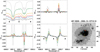 |
Fig. A.1. Hinode/SOT-SP observations at μ = 0.99 of the sunspot AR 10930. Its image at continuum wavelength is shown on the right. We have chosen six pixels, marked using squares on the image, representing different parts of the Sunspot and plotted their Stokes profiles. They sample regions with continuum intensities ranging from the darkest umbra to 0.5 Iqs. The profiles clearly show how the 6301.5 Å and the 6302.5 Å lines become increasingly weaker with decreasing continuum intensity, while at the same time blending by most probably molecular lines increases rapidly. Arrows mark three prominent molecular lines. |
All Tables
Atomic details of the Ti I multiplet at 2.2 μm and two other iron lines (bottom two rows) often used for sunspot diagnostics.
All Figures
|
Fig. 1. Maps of temperature (first row), magnetic field strength (second row), and magnetic field inclination (third row) from the MHD sunspot simulation at log(τ) = 0.0, −0.8, and −2.3. |
| In the text | |
|
Fig. 2. Maps of height of formation of the three lines λ = 6302.5 Å (panel a), 15 648.5 Å (panel b), and 21 897.4 Å (panel c). The height of formation is the centroid of the intensity response function to temperature. Bottom panel: we have plotted the heights of formation along the horizontal black lines, averaging in the y-direction over the narrow region between the two black lines covering four pixels. |
| In the text | |
|
Fig. 3. First and second columns: maps of the equivalent widths and normalized line depths of the intensity profiles. Last columns: maps of maximum circular polarization. All quantities are plotted for four lines the Fe I 6302.5 Å and 1.56 μm lines (top panels), and the Ti I 22 310 Å, and 21 897 Å lines (bottom panels). Contours mark the penumbra-umbra and penumbra-quiet sun boundaries. |
| In the text | |
|
Fig. 4. Stokes I profiles from different features of the sunspot and the quiet Sun. From top to bottom: umbral dots, dark umbral core, penumbral filament head, spine in penumbra, penumbral filament tail, and quiet Sun. At each feature, we show profiles from four sample pixels and indicate the equivalent widths (in mÅ) and normalized line depths. These pixels are at the centers of the squares marked on the images in the last column. The profiles are shown for both the Fe I and the Ti I spectral lines. They are normalized to the spatially averaged quiet Sun continuum intensity (Ic − qs). The contrast on the last column was adapted for better representation of the different features. |
| In the text | |
|
Fig. 5. Stokes Q/Ic profiles from different features of the sunspot and the quiet Sun computed at two iron and two titanium lines. Details are the same as in Fig. 4 but for the Q/Ic − qs profiles. |
| In the text | |
|
Fig. 6. Stokes V/Ic profiles from different features of the sunspot and the quiet Sun computed at two iron and two titanium lines. Details are the same as in Fig. 4 but for V/Ic − qs profiles. |
| In the text | |
|
Fig. 7. Atmospheric maps from the inversion of iron and titanium lines. Left: maps of the temperature (a, e), magnetic field strength (b, f), inclination (c, g), and LOS velocity (d, h) at log(τ) = − 0.8, obtained by inverting the Ti I 21 897 Å (first column) and Fe I 6302 Å (second column) lines. In the LOS velocity maps, blue indicates upflows and red downflows. Right: fit to the degraded Stokes profiles of the Ti and Fe lines at two sample pixels marked on the temperature maps. |
| In the text | |
|
Fig. A.1. Hinode/SOT-SP observations at μ = 0.99 of the sunspot AR 10930. Its image at continuum wavelength is shown on the right. We have chosen six pixels, marked using squares on the image, representing different parts of the Sunspot and plotted their Stokes profiles. They sample regions with continuum intensities ranging from the darkest umbra to 0.5 Iqs. The profiles clearly show how the 6301.5 Å and the 6302.5 Å lines become increasingly weaker with decreasing continuum intensity, while at the same time blending by most probably molecular lines increases rapidly. Arrows mark three prominent molecular lines. |
| In the text | |
Current usage metrics show cumulative count of Article Views (full-text article views including HTML views, PDF and ePub downloads, according to the available data) and Abstracts Views on Vision4Press platform.
Data correspond to usage on the plateform after 2015. The current usage metrics is available 48-96 hours after online publication and is updated daily on week days.
Initial download of the metrics may take a while.