| Issue |
A&A
Volume 653, September 2021
|
|
|---|---|---|
| Article Number | A51 | |
| Number of page(s) | 16 | |
| Section | The Sun and the Heliosphere | |
| DOI | https://doi.org/10.1051/0004-6361/202140847 | |
| Published online | 08 September 2021 | |
Investigation on the spatiotemporal structures of supra-arcade spikes⋆
1
CAS Key Laboratory of Geospace Environment, Department of Geophysics and Planetary Sciences, University of Science and Technology of China, Hefei 230026, PR China
e-mail: rliu@ustc.edu.cn
2
CAS Center for Excellence in Comparative Planetology, University of Science and Technology of China, Hefei 230026, PR China
3
Mengcheng National Geophysical Observatory, University of Science and Technology of China, Mengcheng 233500, PR China
Received:
22
March
2021
Accepted:
8
June
2021
Context. The vertical current sheet (VCS) trailing coronal mass ejections (CMEs) is the key place at which the flare energy release and the CME buildup take place through magnetic reconnection. The VCS is often studied from the edge-on perspective for the morphological similarity with the two-dimensional “standard” picture, but its three-dimensional structure can only be revealed when the flare arcade is observed side on. The structure and dynamics in the so-called supra-arcade region thus contain important clues to the physical processes in flares and CMEs.
Aims. We focus on supra-arcade spikes (SASs), interpreted as the VCS viewed side on, to study their spatiotemporal structures. By comparing the number of spikes and the in situ derived magnetic twist in interplanetary CMEs (ICMEs), we intend to check on the inference from the standard picture that each spike represents an active reconnection site and that each episode of reconnection adds approximately one turn of twist to the CME flux rope.
Methods. For this investigation we selected four events, in which the flare arcade has a significant north-south orientation and the associated CME is traversed by a near-Earth spacecraft. We studied the SASs using high-cadence high-resolution 131 Å images from the Atmospheric Imaging Assembly on board the Solar Dynamics Observatory.
Results. By identifying each individual spike during the decay phase of the selected eruptive flares, we found that the widths of spikes are log-normal distributed. However, the Fourier power spectra of the overall supra-arcade extreme ultraviolet emission, including bright spikes, dark downflows, and the diffuse background, are power-law distributed in terms of either spatial frequency k or temporal frequency ν, which reflects the fragmentation of the VCS. We demonstrate that coronal emission-line intensity observations dominated by Kolmogorov turbulence would exhibit a power spectrum of E(k) ∼ k−13/3 or E(ν) ∼ ν−7/2, which is consistent with our observations. By comparing the number of SASs and the turns of field lines as derived from the ICMEs, we found a consistent axial length of ∼3.5 AU for three events with a CME speed of ∼1000 km s−1 in the inner heliosphere; but we found a much longer axial length (∼8 AU) for the fourth event with an exceptionally fast CME speed of ∼1500 km s−1, suggesting that when the spacecraft traversed its leg this ICME was flattened and its “nose” was significantly past the Earth.
Key words: Sun: flares / Sun: coronal mass ejections (CMEs) / turbulence
Movie associated to Fig. 1 is available at https://www.aanda.org
© ESO 2021
1. Introduction
Magnetic reconnection, a fundamental process in plasma, plays a crucial role in solar flares and coronal mass ejections (CMEs). Numerous theoretical models and numerical simulations have demonstrated the formation of a vertical current sheet (VCS) beneath CMEs (see the review by Lin et al. 2015). In the two-dimensional standard picture (e.g., Kopp & Pneuman 1976; Shibata et al. 1995; Lin & Forbes 2000; Lin et al. 2004), the VCS forms as a rising flux rope stretches the overlying field, which drives a plasma inflow carrying oppositely directed magnetic field into the VCS region. Magnetic reconnection at the VCS turns the overlying, untwisted field lines that constrain the flux rope into twisted field lines that envelope the flux rope. This process strengthens the upward magnetic pressure force while weakening the downward magnetic tension force, therefore leading to the eruption of the flux rope. While adding layers and layers of hot plasma and twisted magnetic flux to the snowballing flux rope, reconnections at the VCS also produce growing flare loops, whose footpoints in the chromosphere are observed as two flare ribbons separating from each other. In the general three-dimensional geometry, the VCS may form at the cross section of two intersecting quasi-separatrix layers, also termed a hyperbolic flux tube, below the flux rope (Titov et al. 2002; Janvier et al. 2015; Liu 2020). In addition to the classic two-ribbon flares, complex magnetic topologies may result in diverse ribbon morphologies, including but not limited to circular ribbons (e.g., Wang & Liu 2012; Chen et al. 2020), X-shaped ribbon (e.g., Liu et al. 2016), and multi-ribbons (e.g., Qiu et al. 2020).
In the era before the launch of the Solar Dynamics Observatory (SDO; Pesnell et al. 2012), the absence of a narrow-band imaging instrument sensitive to hot plasmas above 3 MK made it very difficult to study the VCS. Considerable attention has been given to a coaxial, bright ray feature that appears in coronagraph several hours after some CMEs (e.g., Webb et al. 2003; Lin et al. 2005). Occasionally a bright linear feature in soft X-rays or the extreme ultraviolet (EUV) is observed to extend upward from the top of cusp-shaped flaring loops and line up with the white-light post-CME rays (e.g., Savage et al. 2010; Liu et al. 2010, 2011). In the SDO era, the VCS has been recognized when it is observed edge on (e.g., Liu 2013; Liu et al. 2013; Zhu et al. 2016; Cheng et al. 2018; Warren et al. 2018; Gou et al. 2019), that is, when the morphology can be favorably compared with the standard picture. The VCS has also been noted when it is observed with a face-on perspective (e.g., Warren et al. 2011; Savage et al. 2012a,b; McKenzie 2013; Doschek et al. 2014; Hanneman & Reeves 2014; Innes et al. 2014), that is, when the post-flare arcade is observed from a line of sight (LOS) perpendicular to its axis. In this case, however, supra-arcade downflows (SADs) catch more attention than any other features. These are tadpole-like dark voids falling at a speed ranging from tens to hundreds of kilometers per second through a fan-shaped, haze-like flare plasma above the flare arcade, which is sometimes described as a fan of coronal rays (Švestka et al. 1998) or spike-like rays (McKenzie & Hudson 1999), also referred to as a supra-arcade fan in the literature (Innes et al. 2014; Reeves et al. 2017). Generally, SADs are believed to be a manifestation of reconnection outflows resulting from magnetic reconnection in the VCS.
The VCS must be a three-dimensional structure, which is implied by the post-flare arcade. However, it may not be a continuous slab, extending continuously along the axis of the post-flare arcade, because 1) the arcade consists of numerous discrete post-flare loops (e.g., Jing et al. 2016); 2) the flare ribbons, which are the footpoints of post-flare loops, often consist of discrete kernels in Hα and UV (e.g., Li & Zhang 2015; Lörinčík et al. 2019); and 3) the supra-arcade fan is far from uniform, but the haze-like plasma is often superimposed by multiple spike-like features (e.g, Figs. 1e and f), which are discretely aligned along the top of the arcade and termed supra-arcade spikes (SASs) in this paper. If a post-flare arcade is viewed from an LOS along its axis and there are no prominent coronal features in the foreground or background along the LOS, then the resultant supra-arcade emission must be integrated over the aligned SASs, which gives a linear bright feature extending vertically above the top of the arcade, that is, a typical VCS (e.g., Liu et al. 2010; Cheng et al. 2018). The fan and the SASs are often exclusively observed in the 94 and 131 Å passbands of the Atmospheric Imaging Assembly (AIA; Lemen et al. 2012) on board SDO, which are sensitive to plasmas as hot as ∼6–10 MK (cf. Fig. 1). Plasma heating can be naturally attributed to magnetic reconnection in the VCS.
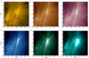 |
Fig. 1. Post-flare arcade observed by different SDO/AIA passbands on 2013 November 7 (Event #3 in Table 1). The panels are arranged in an order of increasing characteristic temperatures of the AIA passbands (O’Dwyer et al. 2010). The SASs are only visible in 94 and 131 Å. An animation of AIA 131 Å images is available online. (a) SDO/AIA 171 Å 2013-11-07T00:25:48.918, (b) SDO/AIA 193 Å 2013-11-07T00:25:45.317, (c) SDO/AIA 211 Å 2013-11-07T00:25:35.624, (d) SDO/AIA 335 Å 2013-11-07T00:25:38.627, (e) SDO/AIA 94 Å 2013-11-07T00:25:37.124, (f) SDO/AIA 94 Å 2013-11-07T00:25:37.124. |
In this work, we carry out an investigation on the spatiotemporal structures of SASs observed during the decay phase of eruptive flares, using high-cadence high-resolution AIA 131 Å images. In the sections that follow, we select four events with typical SAS features (Sect. 2.1) and attempt to identify each spike and estimate its width (Sect. 2.2). We then study the statistical distribution of spike widths (Sect. 3.1) and Fourier power spectra of the supra-arcade EUV emission (Sect. 3.2), discuss the implication for interplanetary CMEs (ICMEs; Sect. 3.3), and finally summarize the major results (Sect. 4).
2. Observation and analysis
2.1. Event selection and overview
We carried out a survey of flares with magnitudes of M class and above in the SDO era to search for events in which the post-flare arcade is viewed side on so that the SASs are visible. To make certain that a magnetic flux rope is involved in the eruption, we required that the associated CME eventually arrives at Earth and is observed as a magnetic cloud (Burlaga et al. 1981; Burlaga 1988) by a near-Earth spacecraft. However, such events are relatively rare because SASs are preferentially visible close to the limb, while it is more probably that CMEs originating from the disk center arrive at Earth than those from near the limb. Eventually we found four events as listed in Table 1; each flare is associated with a halo CME that is observed in situ as an ICME 3–4 days later.
Events.
The SASs are preferentially observed in 131 Å (Fe XXI and Fe XXIII), fairly visible in 94 Å (Fe XVIII) owing to inferior signal-to-noise ratios and cooler characteristic temperatures in this passband, and often invisible in other even cooler passbands of the AIA (Lemen et al. 2012, see Fig. 1) on board the SDO (Pesnell et al. 2012). Hence we focused on the 131 Å passband in this study. The AIA takes full-disk images with a spatial scale of  pixel−1 and a cadence of 12 s. In particular, Fe XXI dominates the 131 Å passband for the flare plasma, with a peak response temperature log T = 7.05, and Fe VIII dominates for the transition region and quiet corona, with a peak response temperature log T = 5.6 (O’Dwyer et al. 2010). Previous studies applying the differential emssion measure technique to the six optically thin passbands of AIA (i.e., 171, 193, 211, 335, 94, 131 Å; cf. Fig. 1) generally demonstrated a significant presence of ∼10 MK plasma above the post-flare arcade (e.g., Gou et al. 2015). Table 1 lists publications that study the supra-arcade plasma of the same flares.
The CMEs were observed by the C2 and C3 coronagraphs of the Large Angle and Spectrometric Coronagraph Experiment (LASCO; Brueckner et al. 1995) on board the Solar and Heliospheric Observatory (SOHO; Domingo et al. 1995). The CME speed in the inner heliosphere (within 30 solar radii) was estimated through a linear fitting to the height-time measurements of the CME front and recorded by the SOHO LASCO CME Catalog1. The ICMEs were detected in situ as they traversed the Wind spacecraft near the Earth. We mainly consulted the ICME list2 compiled by Chi et al. (2016). For each ICME, there could be multiple CME candidates within a time window of 36 h, that is, about 3–4.5 days before the ICME arrival at the Earth, roughly corresponding to an average propagation speed of 400–600 km s−1 between the Sun and Earth. We determined the source of the ICME by carefully taking into account the CME characteristics such as its location, direction, speed, size, and timing. The CME-ICME association for Event #2 has been well established by Vemareddy & Mishra (2015).
2.2. Data analysis
Figures 2–5 show the spikes detected in a typical timescale of 2 h during the flare gradual phase in each of the four events, when the spikes are clearly observed in the AIA 131 Å passband. To detect the spikes, we placed a virtual slit above the post-flare arcade. The slit was either a straight line or a hand-drawn curve to follow the shape of the post-flare arcade (see panel a of each figure). Since the brightness along spikes diminishes with height quickly, we placed the slit not far away from the post-flare arcade. The brightness along the slit is shown in panel b of each figure. A visual inspection indicates that each major peak in this plot corresponds to a spike in the image. We note, however, that these major peaks are superposed by rapid wiggles that are comparable to the measurement errors given by AIA_BP_ESTIMATE_ERROR (shown as error bars). To identify the major peaks but discard the wiggles, we first smoothed the brightness profile along the slit by a five-point running average (shown as the red curve in (b)), and then located the local maximums and minimums in a running box of 13 pixels. All local maximums must exceed 20 DN pixel−1 s−1, an empirical background set in this study. The distance between the two nearest local minimums found at each side of a spike is taken as its width (cf. Sect. 3.1). The identified major peaks are denoted by red arrows on the top of panel b.
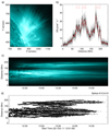 |
Fig. 2. Supra-arcade spikes observed in the 2011 October 22 event. Panel a: snapshot of the flare in the SDO/AIA 131 Å passband. The brightness in units of DN pixel−1 s−1 along a virtual slit (dashed line) is plotted in (b). The starting end of the slit is labeled “0”. In (b) the red curve shows a five-point running average, the error bars indicate the measurement errors given by AIA_BP_ESTIMATE_ERROR, and the red arrows on the top denote the local maximums identified as the spikes. Panel c: evolution of the supra-arcade emission seen through the slit in (a). The identified spikes along the slit are indicated as crosses in (d), which has the same time and distance axes as in (c). (a) AIA 131 Å 22-Oct-2011 13:59:57.620, (b) Slit, (c) Time-Distance Diagram, (d) Identification of Spikes. |
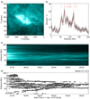 |
Fig. 3. Supra-arcade spikes observed in the 2013 April 11 event. The panels are shown in the same format as in Fig. 2. (a) AIA 131 Å 11-Apr-2013 07:53:56.620, (b) Slit, (c) Time-Distance Diagram, (d) Identification of Spikes. |
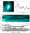 |
Fig. 4. Supra-arcade spikes observed in the 2013 November 7 event. The panels are shown in the same format as in Fig. 2. (a) AIA 131 Å 7-Nov-2013 00:25:44.620, (b) Slit, (c) Time-Distance Diagram, (d) Identification of Spikes. |
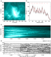 |
Fig. 5. Supra-arcade spikes observed in the 2014 April 2 event. The panels are shown in the same format as in Fig. 2. (a) AIA 131 Å 2-Apr-2014 14:28:44.620, (b) Slit, (c) Time-Distance Diagram, (d) Identification of Spikes. |
Further, for the two disk events, #2 and #4, AIA 131 Å images are co-registered to the first image taken during each selected time interval using the SSW procedure DROT_MAP. We made the time-distance stack plot (panel c) by taking a slice along the virtual slit from each image and then arranging the slices in chronological order. The temporal evolution of spikes was then recorded in this time-distance diagram. We can see that some spikes evolve consistently, some are wavering due to SADs, and others may apparently appear or disappear during the investigated time period. It is interesting that some SADs reveal themselves as dark, tadpole-like features in the time-distance diagram as they propagate through the slit (e.g., Fig. 2c). It can be seen that SADs may not only flow along intra-spike channels but also into the spikes, the latter of which may result in the apparent splitting of a spike (some clear examples can be seen in Fig. 3c). Such interactions between bright spikes and dark down-flowing voids are suggested to be evidence for Rayleigh-Taylor type instabilities in the exhaust of reconnection jets (Guo et al. 2014; Innes et al. 2014).
The identified spikes along the slit are plotted as crosses in panel d, which has the same time and distance axes as the time-distance diagram in panel c. We find our identification algorithm to be satisfying though a visual comparison between panels c and d. The time-averaged number of spikes and the standard deviation are annotated on the top right of panel d.
3. Discussion
3.1. Distribution of spike widths
Because we estimated the width of each spike (Sect. 2.2), we now plot the distribution of spike widths during the gradual phase of each flare (Fig. 6). The distribution of all four flares investigated is rather similar, with a peak at around 5–6 Mm, an average of 16–21 Mm, a standard deviation of 7–11 Mm, and a median of 15–19 Mm. The peak of 5–6 Mm is very consistent with the current-sheet width detected in the lower corona in EUV passbands as reported in the literature (e.g., Liu et al. 2010; Zhu et al. 2016). Each distribution also has a similar lower cutoff of about 3 Mm and an upper limit of about 20 Mm. The lower cutoff can be attributed to the running box of 13 pixels specified in our algorithm, which effectively limits the spike width to be above 6 pixels, or 2.6 Mm. This is smaller than the lower limit of the current-sheet width, 3 Mm, deduced by Guo et al. (2013) from the nonlinear scaling law of the plasmoid instability. We note that Lin et al. (2007, 2009) gave a larger lower limit (50 Mm) based on the linear scaling law.
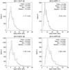 |
Fig. 6. Distribution of the widths of SASs. Each panel shows the histogram for one of the four events under investigation. The statistics of the distribution are indicated in the top right, and the fitting parameters (μ, σ) of the log-normal function (Eq. (1)) in the middle right. The fitting function is plotted as a dashed curve. |
Apparently, spike widths are log-normally, rather than normally, distributed. In Fig. 6, employing a nonlinear least squares fitting procedure MPFIT3 (Markwardt et al. 2009) and assuming a two-pixel measurement error, we fit each distribution with the following function:
![$$ \begin{aligned} y(x)=\frac{C}{x\sigma \sqrt{2\pi }}\exp \left[-\frac{(\ln x -\mu )^2}{2\sigma ^2}\right], \end{aligned} $$](/articles/aa/full_html/2021/09/aa40847-21/aa40847-21-eq2.gif)
where C is an arbitrary constant. The other two parameters (μ, σ) are annotated in the middle right of each panel. It is noteworthy that we obtain similar μ and σ in all four events.
3.2. Spatiotemporal structures of supra-arcade EUV emission
We apply the Fourier transform to each vertical slice in the time-distance diagram in panel c of Figs. 2–5 to explore the structure of the supra-arcade emission in terms of spatial frequency k (Mm−1). We fit the Fourier power spectrum resulting from each vertical slice with a power-law function and show the temporal variation of the power-law index γs in the left column of Fig. 7. Collapsing the time-distance diagram along the time axis gives the time-integrated EUV emission profile along the slit. Applying the Fourier transform to this profile, we obtain power spectra exhibiting clear power-law behaviors (right column of Fig. 7), whose fitted indices are in the range ∼[4, 5], similar to the range of γs in the left column.
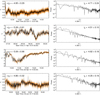 |
Fig. 7. Structure of supra-arcade EUV emission in terms of spatial frequency. The power spectrum of any vertical slice in the time-distance diagram (panel c of Figs. 2–5) is fitted with a power-law function. The temporal variation of the power-law index γs is shown in the left panels. The orange bars indicate the 1σ uncertainty estimates in the fittings. The power spectrum of the time-distance diagram collapsed along the time axis is shown in the right panels. |
Similarly, we apply the Fourier transform to each horizontal slice in the time-distance diagram in panel c of Figs. 2–5 to explore the structure of the supra-arcade emission in terms of temporal frequency ν (mHz). Fitting the Fourier power spectrum from each horizontal slice by a power-law function, we show the variation of the resultant power-law index γt along the virtual slit in the left column of Fig. 8. Collapsing the time-distance diagram along the distance axis, we effectively integrate the EUV emission along the slit, which emulates the situation when the VCS is observed edge on in the optically thin corona. This results in a time series of EUV emission sampled from a point on the VCS. The power spectra of spatially integrated EUV emission also exhibit clear power-law shapes (right column of Fig. 8), whose indices are in the range ∼[2.5, 4], similar to the range of γt in the left column.
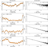 |
Fig. 8. Structure of supra-arcade EUV emission in terms of temporal frequency. The power spectrum of any horizontal slice in the time-distance diagram (panel c of Figs. 2–5) is fitted with a power-law function. The spatial variation of the power-law index γt along each slit (panel a in Figs. 2–5) is shown in the left panels. The orange bars indicate the 1σ uncertainty estimates in the fittings. The power spectrum of the time-distance diagram collapsed along the distance axis is shown in the right panels. |
Cheng et al. (2018) construct time-distance diagrams from a slit along a VCS observed edge on. Sampling two horizontal slices above the flare arcade in a time-distance diagram, these authors obtained the corresponding Fourier power spectra with a power-law indices α of 1.8 and 1.2, respectively. The difference in power-law indices between γt in our case and α in Cheng et al. (2018) can probably be attributed to the following differences: First, the power spectra in Cheng et al. (2018) appear very noisy (their Fig. 13), lacking a strict power-law shape, compared with the nice power-law behavior demonstrated in Figs. 7 and 8. Second, the LOS integration in their case includes the coronal foreground and background, whereas in our case the spatial integration is limited to coronal emission right above the post-flare arcade and therefore there are fewer interferences from irrelevant coronal structures.
Below we demonstrate heuristically the consistency of the observed power-law behavior with Kolmogorov turbulence in the supra-arcade region. Any turbulent physical quantity can be written as

where u0(x, t) varies smoothly at large spatiotemporal scales, while δu(x, t) fluctuates randomly at small scales, that is, there is a large separation of space and time scales between the mean and fluctuating components. The two components hence respond distinctively to a long wavelength average, that is,

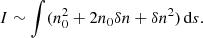
The Fourier transform of the observed intensity I = I0 + δI gives the power spectra

in terms of spatial frequency k and temporal frequency ν, respectively, as shown in Figs. 7 and 8. Here for clarity, the spectral index γs and γt are set as positive; I0 is transformed to the low-frequency end of the power spectra; and δI to the higher-frequency portion with power-law behavior, that is,  , which gives
![$$ \begin{aligned} \delta I \sim l^{\,(\gamma _s-1)/2} \sim l^{\,[3/2,\ 2]}, \end{aligned} $$](/articles/aa/full_html/2021/09/aa40847-21/aa40847-21-eq7.gif)
because γs is found to be in the range [4, 5]. Similarly, since δI2 ∼ E(ν)ν, we have
![$$ \begin{aligned} \delta I \sim \nu ^{-(\gamma _t-1)/2} \sim \nu ^{-[3/4,\ 3/2]}, \end{aligned} $$](/articles/aa/full_html/2021/09/aa40847-21/aa40847-21-eq8.gif)
with γt in the range [2.5, 4].
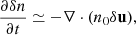
On the other hand, the intensity of coronal emission lines I ∼ ∫n2ds (Aschwanden 2005, Sect. 2.8), where s is the distance along the LOS. Expanding n according to Eq. (2), we have
The LOS integration a priori takes a long wavelength average, which gives
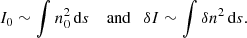
As a comparison, we anticipate that the turbulent component would be smoothened out in white-light observations of the K-corona, in which the observed intensity is dominated by Thomson scattering, that is, I ∼ ∫nds.
The density perturbation δn is linked to the velocity fluctuation δu by the equation of continuation
assuming that |δn| ≪ n0 but |∂n0/∂t| ≪ |∂δn/∂t| and u0 ≃ 0. Thus,
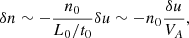
in orders of magnitude, where t0 and L0 are characteristic time and length scale of the system, respectively. The assumption that the Alfvén speed VA is on the same order of magnitude as L0/t0 implies that |δu| ≪ VA. This is consistent with spectroscopic observations of hot emission lines in the VCS, which give nonthermal velocities of no larger than 200 km s−1 (e.g., Li et al. 2018). We further argue that the LOS integration from the side-on perspective of the VCS make relevant the size l of large eddies in the flow velocity field u ≃ δu, where the thickness of the VCS is comparable to those of spikes; that is, δI ∼ δu2 l, where l ≲ L0. l can be deemed as the order of magnitude of distances over which δu changes appreciably.
If the observed intensity perturbations δI result from a fully developed turbulence following the famous universal law of Kolmogorov and Obukhov (i.e.,  ) (Landau & Lifshitz 1987, Sect. 33), then we have

The index 5/3 falls nicely in the compact range [3/2, 2] as given independently by Eq. (5). With ν ∼ (l δu)−1 ∼ l−4/3, we have

in which the index also falls in the compact range [3/4, 3/2] as given by Eq. (6).
Thus, when the fluctuations in coronal emission-line intensity observations are dominated by turbulence, the corresponding power spectra are expected to exhibit the power-law behavior as follows,

As a further evidence of turbulence in the VCS region, we can see from the left column of Fig. 8 that the power-law index γt is generally closer to the value of 7/2 in the middle of the slit, that is, within the VCS region, than at the two ends of the slit, that is, outside of the VCS.
In contrast, the LOS integration from the edge-on perspective of the VCS gives δI ∼ δu2 L, where the depth of the VCS is comparable to the axial length of the post-flare arcade (i.e., L ≫ L0). This leads to power spectra in k−7/3 or ν−2, which are only slightly steeper than those obtained by Cheng et al. (2018).
3.3. Implication for ICMEs
Each SAS can be considered as a reconnection site on the 3D VCS in the wake of the CME. According to the standard model, each episode of magnetic reconnection of the overlying field at the VCS adds a twist of roughly one turn to the burgeoning CME flux rope. If magnetic reconnections at each SAS proceeds continually, that is, there is no significant time interval between any two episodes of magnetic reconnection on the same SAS, then at any time we may assume that the number of ongoing reconnection episodes roughly correspond to the number of SASs. Since the number of SASs is stable during the flare decay phase, we expect that the outer shells of the flux rope are more or less uniformly twisted (e.g., Wang et al. 2017). When the CME arrives at the Earth, we would expect near-Earth spacecrafts to detect a magnetic cloud possessing magnetic twist of similar number of turns in its outer shells as the number of SASs.
We fit the four ICMEs by a uniform-twist, force-free flux rope model that takes into account the plasma motion (Wang et al. 2016). The in situ observations and corresponding fitting results are shown in Figs. A.1–A.4. The model yields the twist density τ = rBϕ/Bz in local cylindrical coordinates (r, ϕ, z) with the z-axis directed along the flux-rope axis. The τ is given in units of the number of field line turns per unit AU along the flux-rope axis. The helicity (twist) signs are negative for all four events, which, except Event #3, originate from the northern hemisphere, which is consistent with the cycle-independent dominance of negative helicity in the same hemisphere (Zhou et al. 2020, and references therein). Event #3 originates from a decayed active region (AR 11882) in the southern hemisphere close to the equator. When it is located near the disk center, the active region exhibits a weak reverse-S geometry manifested by coronal loops in EUV (Fig. 9c), associated with a filament aligned along the polarity inversion line with a similar geometry, signaling the presence of negative helicity. In contrast, AR 11314, the source region of Event #1 exhibits a forward-S geometry in the east and a reverse-S geometry in the west (Fig. 9a), suggesting that the CME probably originates from the west side of the active region. The other two source regions, ARs 11719 (Fig. 9b) and 12027 (Fig. 9d), are clearly reverse-S shaped; the latter is outlined by a sigmoidal filament. Additionally, different aspects of the source region of Event #2, AR 11719, has been studied in detail by several authors (Vemareddy & Mishra 2015; Vemareddy et al. 2016; Guo et al. 2019).
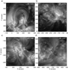 |
Fig. 9. Four active regions under investigation as observed by SDO/AIA. (a) AIA 193 Å 2011-10-16T21:30:43, (b) AIA 94 Å 2013-04-11T06:00:37, (c) AIA 193 Å 2013-10-31T22:00:42, (d) AIA 193 Å 2014-04-02T13:00:42. |
The axial length of the ICME is unknown but assumed to be lie in the range 2–π AU. At the lower end, the flux rope is so stretched that it is “folded” in half between the Sun and Earth; but at the higher end, the rope is circular (Wang et al. 2015). Alternatively, Hu et al. (2015) compared the lengths of ICME field lines that are derived from energetic electron bursts observed at 1 AU and the magnetic twist derived from the Grad-Shafranov reconstruction method. These authors concluded that the effective axial lengths of the selected ICME events range between 2 AU and 4 AU. Unfortunately none of our selected events is associated with in situ energetic electron bursts. However, the comparison between the number of SASs and the magnetic twist of ICMEs as below may shed new light onto their axial lengths.
In the first three events, we found that τ linearly increases with the increasing number of SASs (left panel of Fig. 10). Further, the ratio of the number of SASs to τ gives a similar length of the flux-rope axis(i.e., ∼3.5 AU; middle panel of Fig. 10), which is slightly above π AU, but still falls in the range suggested by Hu et al. (2015). However, the fourth event seem to be an outlier: this is the only event originating from close to the east limb (about 60° east), but the resultant ICME is still “skimmed” by the near-Earth spacecraft for over 30 h (Fig. A.4), indicating its large size; the ICME has a moderate τ but the number of SASs is the largest among the four events, which is translated to an axial length of 8.3 AU. These may be caused by two different but interrelated effects, both resulting from its exceptionally fast speed (∼1500 km s−1 projected on the plane of sky) as measured in the inner heliosphere by SOHO/LASCO.
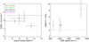 |
Fig. 10. Implication of the number of SASes for ICMEs. Left panel: twist density τ of ICMEs vs. the number of spikes. The error bars for the former are given by the fitting of ICMEs with a uniformly twisted flux-rope model (see the text for details), and those for the latter are the standard deviations of the average number of spikes detected during the selected time intervals during the flare decay phase of each event. Right panel: ratio of the number of spikes over τ in relation to the CME speed estimated in the inner heliosphere. The error bars are given by the propagation of uncertainties. |
First, the ICME experiences a much stronger resistance than the other three events when it “plows” through the solar wind, since in principle the aerodynamic drag force applied on the ICME is proportional to the square of the difference between the ICME speed and the solar wind speed (Cargill 2004). Hence the drag force acting on the fourth ICME is roughly 3.5 times more than that on the other three, given the solar wind speed in the range 400–450 km s−1. The resistance restricts the ICME radial much more than its lateral expansion (e.g., Manchester et al. 2004). However, this would lead to an unrealistically highly flattened shape (right panel of Fig. 10) if the spacecraft crossed the nose of the flux rope. We then suggest that the spacecraft actually traverses the leg of the ICME, which is evidenced by its axis being oriented almost along the Sun-Earth line (Table 1). As a comparison, the flux-rope axes in the other three events make large angles with respect to the Sun-Earth line. Hence at the time of the spacecraft passing, the nose of the fourth ICME is significantly past the Earth, resulting in an axial length much longer than π AU. However, if the axis has a circular shape, the nose of the ICME would be over 2.5 AU from the Sun. This is translated to an average propagation speed of ∼1300 km s−1, which is also unrealistic. In reality, we may be witnessing a combination of both the flattening and the leg-passing effect.
Wang et al. (2016) converted the field-line length Lmfl estimated by the electron-probe method in seven magnetic clouds from Kahler et al. (2011) to a twist density τe based on the uniformly twisted Gold-Hoyle flux rope model (Gold & Hoyle 1960) (i.e., 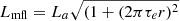 ), assuming that the flux-rope axial length La is in the range 2–π AU. A good correlation is found between τe and τ except for an outlier with an exceptionally large τe exceeding 10 turns AU−1. This could result from an underestimated La, in light of our Event #4, whose estimated axial length greatly exceeds π AU.
4. Conclusions
To summarize, we investigated the SASs observed during the decay phase of four selected eruptive flares, using high-cadence high-resolution AIA 131 Å images. By identifying each individual spike, we find that the spike widths are log-normally distributed. The distribution has a lower cutoff at 2.6 Mm owing to our identification algorithm. On the other hand, the Fourier power spectra of the overall supra-arcade EUV emission, including spikes, downflows, and haze, are power-law distributed, in terms of both spatial and temporal frequencies up to ∼0.7 Mm−1 and ∼40 mHz, respectively. Further, assuming that each spike represents an active reconnection site on the three-dimensional VCS, we compare the number of SASs with the turns of field lines as derived from the ICMEs. The comparison gives a consistent axial length of ∼3.5 AU for three events with a CME speed of ∼1000 km s−1 in the inner heliosphere, but a much longer axial length (∼8 AU) for the fourth event with a CME speed of ∼1500 km s−1, which may be a consequence of a combination of the flattening and leg-crossing effect.
The power-law behavior of the supra-arcade power spectra demonstrates the absence of a dominant spatio-temporal scale in the supra-arcade region, and furthermore, the power-law indices are consistent with Kolmogrov turbulence developed in the VCS (see also Freed & McKenzie 2018; Cheng et al. 2018), probably resulting from, for example, plasmoid instability (Loureiro & Uzdensky 2016). It is clear from the side-on perspective that not only the bright spikes but also diffuse background and dark voids collectively contribute to the power-law behavior. The widths of spikes are log-normally distributed, which might be a signature of the fragmentation of the VCS, since the log-normal distribution is known to be able to closely describe the size distribution in a wide variety of fragmentation phenomena (e.g., Kolmogorov 1941; Cheng & Redner 1988; Brown 1989). In addition, to verify the axial length as inferred from the ratio of the number of SASs to the ICME twist density, we need look for further constraints, such as those from interplanetary energetic electrons or multi-spacecraft observations, in future investigations.
Movie
Movie 1 associated with Fig. 1 Access here
Acknowledgments
This work was supported by the Strategic Priority Program of the Chinese Academy of Sciences (XDB41030100) and the National Natural Science Foundation of China (NSFC; 41774150 and 11925302).
References
- Aschwanden, M. J. 2005, Physics of the Solar Corona. An Introduction with Problems and Solutions, 2nd edn. (Chichester, UK; Springer, New York, Berlin: Praxis Publishing Ltd.) [Google Scholar]
- Brown, W. K. 1989, JApA, 10, 89 [NASA ADS] [Google Scholar]
- Brueckner, G. E., Howard, R. A., Koomen, M. J., et al. 1995, Sol. Phys., 162, 357 [NASA ADS] [CrossRef] [Google Scholar]
- Burlaga, L. F. 1988, J. Geophys. Res., 93, 7217 [NASA ADS] [CrossRef] [Google Scholar]
- Burlaga, L., Sittler, E., Mariani, F., & Schwenn, R. 1981, J. Geophys. Res., 86, 6673 [Google Scholar]
- Cargill, P. J. 2004, Sol. Phys., 221, 135 [NASA ADS] [CrossRef] [Google Scholar]
- Chen, X., Liu, R., Deng, N., & Wang, H. 2017, A&A, 606, A84 [NASA ADS] [CrossRef] [EDP Sciences] [Google Scholar]
- Chen, J., Liu, R., Liu, K., et al. 2020, ApJ, 890, 158 [Google Scholar]
- Cheng, Z., & Redner, S. 1988, Phys. Rev. Lett., 60, 2450 [NASA ADS] [CrossRef] [Google Scholar]
- Cheng, X., Li, Y., Wan, L. F., et al. 2018, ApJ, 866, 64 [NASA ADS] [CrossRef] [Google Scholar]
- Chi, Y., Shen, C., Wang, Y., et al. 2016, Sol. Phys., 291, 2419 [NASA ADS] [CrossRef] [Google Scholar]
- Domingo, V., Fleck, B., & Poland, A. I. 1995, Sol. Phys., 162, 1 [NASA ADS] [CrossRef] [Google Scholar]
- Doschek, G. A., McKenzie, D. E., & Warren, H. P. 2014, ApJ, 788, 26 [CrossRef] [Google Scholar]
- Freed, M. S., & McKenzie, D. E. 2018, ApJ, 866, 29 [NASA ADS] [CrossRef] [Google Scholar]
- Gold, T., & Hoyle, F. 1960, MNRAS, 120, 89 [NASA ADS] [Google Scholar]
- Gou, T., Liu, R., & Wang, Y. 2015, Sol. Phys., 290, 2211 [NASA ADS] [CrossRef] [Google Scholar]
- Gou, T., Liu, R., Kliem, B., Wang, Y., & Veronig, A. M. 2019, Sci. Adv., 5, 7004 [Google Scholar]
- Guo, L.-J., Bhattacharjee, A., & Huang, Y.-M. 2013, ApJ, 771, L14 [CrossRef] [Google Scholar]
- Guo, L. J., Huang, Y. M., Bhattacharjee, A., & Innes, D. E. 2014, ApJ, 796, L29 [NASA ADS] [CrossRef] [Google Scholar]
- Guo, J., Wang, H., Wang, J., et al. 2019, ApJ, 874, 181 [NASA ADS] [CrossRef] [Google Scholar]
- Hanneman, W. J., & Reeves, K. K. 2014, ApJ, 786, 95 [NASA ADS] [CrossRef] [Google Scholar]
- Hu, Q., Qiu, J., & Krucker, S. 2015, J. Geophys. Res. (Space Phys.), 120, 5266 [NASA ADS] [CrossRef] [Google Scholar]
- Innes, D. E., Guo, L. J., Bhattacharjee, A., Huang, Y. M., & Schmit, D. 2014, ApJ, 796, 27 [NASA ADS] [CrossRef] [Google Scholar]
- Janvier, M., Aulanier, G., & Démoulin, P. 2015, Sol. Phys., 290, 3425 [NASA ADS] [CrossRef] [Google Scholar]
- Jing, J., Xu, Y., Cao, W., et al. 2016, Sci. Rep., 6, 24319 [NASA ADS] [CrossRef] [Google Scholar]
- Kahler, S. W., Krucker, S., & Szabo, A. 2011, J. Geophys. Res. (Space Phys.), 116, A01104 [Google Scholar]
- Kolmogorov, A. N. 1941, in Dokl Akad. Nauk. SSSR, 99 [Google Scholar]
- Kopp, R. A., & Pneuman, G. W. 1976, Sol. Phys., 50, 85 [NASA ADS] [CrossRef] [Google Scholar]
- Landau, L. D., & Lifshitz, E. M. 1987, Fluid Mechanics, 2nd edn. (Butterworth-Heinemann publications) [Google Scholar]
- Lemen, J. R., Title, A. M., Akin, D. J., et al. 2012, Sol. Phys., 275, 17 [Google Scholar]
- Li, T., & Zhang, J. 2015, ApJ, 804, L8 [NASA ADS] [CrossRef] [Google Scholar]
- Li, Y., Xue, J. C., Ding, M. D., et al. 2018, ApJ, 853, L15 [Google Scholar]
- Lin, J., & Forbes, T. G. 2000, J. Geophys. Res., 105, 2375 [NASA ADS] [CrossRef] [Google Scholar]
- Lin, J., Raymond, J. C., & van Ballegooijen, A. A. 2004, ApJ, 602, 422 [NASA ADS] [CrossRef] [Google Scholar]
- Lin, J., Ko, Y. K., Sui, L., et al. 2005, ApJ, 622, 1251 [NASA ADS] [CrossRef] [Google Scholar]
- Lin, J., Li, J., Forbes, T. G., et al. 2007, ApJ, 658, L123 [NASA ADS] [CrossRef] [Google Scholar]
- Lin, J., Li, J., Ko, Y.-K., & Raymond, J. C. 2009, ApJ, 693, 1666 [NASA ADS] [CrossRef] [Google Scholar]
- Lin, J., Murphy, N. A., Shen, C., et al. 2015, Space Sci. Rev., 194, 237 [NASA ADS] [CrossRef] [Google Scholar]
- Liu, R. 2013, MNRAS, 434, 1309 [NASA ADS] [CrossRef] [Google Scholar]
- Liu, R. 2020, Res. Astron. Astrophys., 20, 165 [Google Scholar]
- Liu, R., Lee, J., Wang, T., et al. 2010, ApJ, 723, L28 [NASA ADS] [CrossRef] [Google Scholar]
- Liu, R., Wang, T.-J., Lee, J., et al. 2011, Res. Astron. Astrophys., 11, 1209 [CrossRef] [Google Scholar]
- Liu, W., Chen, Q., & Petrosian, V. 2013, ApJ, 767, 168 [NASA ADS] [CrossRef] [Google Scholar]
- Liu, R., Chen, J., Wang, Y., & Liu, K. 2016, Sci. Rep., 6, 34021 [CrossRef] [Google Scholar]
- Lörinčík, J., Aulanier, G., Dudík, J., Zemanová, A., & Dzifčáková, E. 2019, ApJ, 881, 68 [Google Scholar]
- Loureiro, N. F., & Uzdensky, D. A. 2016, Plasma Phys. Control. Fusion, 58 [Google Scholar]
- Manchester, W. B., Gombosi, T. I., Roussev, I., et al. 2004, J. Geophys. Res. (Space Phys.), 109, A02107 [Google Scholar]
- Markwardt, C. B. 2009, in Astronomical Data Analysis Software and Systems XVIII, eds. D. A. Bohlender, D. Durand, & P. Dowler, ASP Conf. Ser., 411, 251 [Google Scholar]
- McKenzie, D. E. 2013, ApJ, 766, 39 [NASA ADS] [CrossRef] [Google Scholar]
- McKenzie, D. E., & Hudson, H. S. 1999, ApJ, 519, L93 [NASA ADS] [CrossRef] [Google Scholar]
- O’Dwyer, B., Del Zanna, G., Mason, H. E., Weber, M. A., & Tripathi, D. 2010, A&A, 521, A21 [NASA ADS] [CrossRef] [EDP Sciences] [Google Scholar]
- Pesnell, W. D., Thompson, B. J., & Chamberlin, P. C. 2012, Sol. Phys., 275, 3 [Google Scholar]
- Qiu, Y., Guo, Y., Ding, M., & Zhong, Z. 2020, ApJ, 901, 13 [NASA ADS] [CrossRef] [Google Scholar]
- Reeves, K. K., Freed, M. S., McKenzie, D. E., & Savage, S. L. 2017, ApJ, 836, 55 [NASA ADS] [CrossRef] [Google Scholar]
- Samanta, T., Tian, H., Chen, B., et al. 2021, The Innovation, 2 [Google Scholar]
- Savage, S. L., McKenzie, D. E., Reeves, K. K., Forbes, T. G., & Longcope, D. W. 2010, ApJ, 722, 329 [NASA ADS] [CrossRef] [Google Scholar]
- Savage, S. L., Holman, G., Reeves, K. K., et al. 2012a, ApJ, 754, 13 [Google Scholar]
- Savage, S. L., McKenzie, D. E., & Reeves, K. K. 2012b, ApJ, 747, L40 [NASA ADS] [CrossRef] [Google Scholar]
- Scott, R. B., McKenzie, D. E., & Longcope, D. W. 2016, ApJ, 819, 56 [Google Scholar]
- Shibata, K., Masuda, S., Shimojo, M., et al. 1995, ApJ, 451, L83 [Google Scholar]
- Švestka, Z., Fárník, F., Hudson, H. S., & Hick, P. 1998, Sol. Phys., 182, 179 [NASA ADS] [CrossRef] [Google Scholar]
- Titov, V. S., Hornig, G., & Démoulin, P. 2002, J. Geophys. Res. (Space Phys.), 107, 1164 [NASA ADS] [CrossRef] [Google Scholar]
- Vemareddy, P., & Mishra, W. 2015, ApJ, 814, 59 [CrossRef] [Google Scholar]
- Vemareddy, P., Möstl, C., Amerstorfer, T., et al. 2016, ApJ, 828, 12 [NASA ADS] [CrossRef] [Google Scholar]
- Wang, H., & Liu, C. 2012, ApJ, 760, 101 [Google Scholar]
- Wang, Y., Zhou, Z., Shen, C., Liu, R., & Wang, S. 2015, J. Geophys. Res. (Space Phys.), 120, 1543 [Google Scholar]
- Wang, Y., Zhuang, B., Hu, Q., et al. 2016, J. Geophys. Res. (Space Phys.), 121, 9316 [NASA ADS] [CrossRef] [Google Scholar]
- Wang, W., Liu, R., Wang, Y., et al. 2017, Nat. Commun., 8, 1330 [NASA ADS] [CrossRef] [Google Scholar]
- Warren, H. P., O’Brien, C. M., & Sheeley, N. R., Jr. 2011, ApJ, 742, 92 [Google Scholar]
- Warren, H. P., Brooks, D. H., Ugarte-Urra, I., et al. 2018, ApJ, 854, 122 [CrossRef] [Google Scholar]
- Webb, D. F., Burkepile, J., Forbes, T. G., & Riley, P. 2003, J. Geophys. Res. (Space Phys.), 108, 1440 [NASA ADS] [CrossRef] [Google Scholar]
- Xue, J., Su, Y., Li, H., & Zhao, X. 2020, ApJ, 898, 88 [CrossRef] [Google Scholar]
- Zhou, Z., Liu, R., Cheng, X., et al. 2020, ApJ, 891, 180 [CrossRef] [Google Scholar]
- Zhu, C., Liu, R., Alexander, D., & McAteer, R. T. J. 2016, ApJ, 821, L29 [NASA ADS] [CrossRef] [Google Scholar]
Appendix A: Supplementary figures
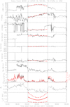 |
Fig. A.1. In situ observation of the ICME resulting from the 2011 October 22 solar event. Shown from top to bottom are the magnetic field magnitude B, field inclination angle θ (with respect to the ecliptic plane), azimuthal angle ϕ (0 deg pointing to the Sun), three components (Vx, Vy, Vz) of the solar wind velocity in the GSE coordinate system, proton density Np, proton temperature Tp (superimposed by Tp/Texp, where Texp is an empirical temperature determined from solar wind speed), plasma β, and half of the field-line length assuming that the flux-rope axial length is in the range 2–π AU. The dashed red curves show the model fitting results with the uniformly twisted flux-rope (Gold-Hoyle) solution. The closest approach of the observational path to the flux-rope axis d is 0.37 in terms of the rope radius; the goodness of fit χn is 0.21, which is the normalized root mean square of the difference between the fitting and observation. |
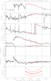 |
Fig. A.2. In situ observation of the ICME resulting from the 2013 April 11 solar event. Shown from top to bottom are magnetic field magnitude B, field inclination angle θ, azimuthal angle ϕ (0 deg pointing to the Sun), and three components (Vx, Vy, Vz) of the solar wind velocity in the GSE coordinate system. The closest approach d = 0.60, and the goodness of fit χn = 0.18. |
 |
Fig. A.3. In situ observation of the ICME resulting from the 2013 November 7 solar event. The panels are shown in the same format as in Fig. A.2. The closest approach d = 0.23, and the goodness of fit χn = 0.19. |
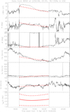 |
Fig. A.4. In situ observation of the ICME resulting from the 2014 April 2 solar event. The panels are shown in the same format as in Fig. A.2. The closest approach d = 0.88, and the goodness of fit χn = 0.33. |
All Tables
All Figures
|
Fig. 1. Post-flare arcade observed by different SDO/AIA passbands on 2013 November 7 (Event #3 in Table 1). The panels are arranged in an order of increasing characteristic temperatures of the AIA passbands (O’Dwyer et al. 2010). The SASs are only visible in 94 and 131 Å. An animation of AIA 131 Å images is available online. (a) SDO/AIA 171 Å 2013-11-07T00:25:48.918, (b) SDO/AIA 193 Å 2013-11-07T00:25:45.317, (c) SDO/AIA 211 Å 2013-11-07T00:25:35.624, (d) SDO/AIA 335 Å 2013-11-07T00:25:38.627, (e) SDO/AIA 94 Å 2013-11-07T00:25:37.124, (f) SDO/AIA 94 Å 2013-11-07T00:25:37.124. |
| In the text | |
|
Fig. 2. Supra-arcade spikes observed in the 2011 October 22 event. Panel a: snapshot of the flare in the SDO/AIA 131 Å passband. The brightness in units of DN pixel−1 s−1 along a virtual slit (dashed line) is plotted in (b). The starting end of the slit is labeled “0”. In (b) the red curve shows a five-point running average, the error bars indicate the measurement errors given by AIA_BP_ESTIMATE_ERROR, and the red arrows on the top denote the local maximums identified as the spikes. Panel c: evolution of the supra-arcade emission seen through the slit in (a). The identified spikes along the slit are indicated as crosses in (d), which has the same time and distance axes as in (c). (a) AIA 131 Å 22-Oct-2011 13:59:57.620, (b) Slit, (c) Time-Distance Diagram, (d) Identification of Spikes. |
| In the text | |
|
Fig. 3. Supra-arcade spikes observed in the 2013 April 11 event. The panels are shown in the same format as in Fig. 2. (a) AIA 131 Å 11-Apr-2013 07:53:56.620, (b) Slit, (c) Time-Distance Diagram, (d) Identification of Spikes. |
| In the text | |
|
Fig. 4. Supra-arcade spikes observed in the 2013 November 7 event. The panels are shown in the same format as in Fig. 2. (a) AIA 131 Å 7-Nov-2013 00:25:44.620, (b) Slit, (c) Time-Distance Diagram, (d) Identification of Spikes. |
| In the text | |
|
Fig. 5. Supra-arcade spikes observed in the 2014 April 2 event. The panels are shown in the same format as in Fig. 2. (a) AIA 131 Å 2-Apr-2014 14:28:44.620, (b) Slit, (c) Time-Distance Diagram, (d) Identification of Spikes. |
| In the text | |
|
Fig. 6. Distribution of the widths of SASs. Each panel shows the histogram for one of the four events under investigation. The statistics of the distribution are indicated in the top right, and the fitting parameters (μ, σ) of the log-normal function (Eq. (1)) in the middle right. The fitting function is plotted as a dashed curve. |
| In the text | |
|
Fig. 7. Structure of supra-arcade EUV emission in terms of spatial frequency. The power spectrum of any vertical slice in the time-distance diagram (panel c of Figs. 2–5) is fitted with a power-law function. The temporal variation of the power-law index γs is shown in the left panels. The orange bars indicate the 1σ uncertainty estimates in the fittings. The power spectrum of the time-distance diagram collapsed along the time axis is shown in the right panels. |
| In the text | |
|
Fig. 8. Structure of supra-arcade EUV emission in terms of temporal frequency. The power spectrum of any horizontal slice in the time-distance diagram (panel c of Figs. 2–5) is fitted with a power-law function. The spatial variation of the power-law index γt along each slit (panel a in Figs. 2–5) is shown in the left panels. The orange bars indicate the 1σ uncertainty estimates in the fittings. The power spectrum of the time-distance diagram collapsed along the distance axis is shown in the right panels. |
| In the text | |
|
Fig. 9. Four active regions under investigation as observed by SDO/AIA. (a) AIA 193 Å 2011-10-16T21:30:43, (b) AIA 94 Å 2013-04-11T06:00:37, (c) AIA 193 Å 2013-10-31T22:00:42, (d) AIA 193 Å 2014-04-02T13:00:42. |
| In the text | |
|
Fig. 10. Implication of the number of SASes for ICMEs. Left panel: twist density τ of ICMEs vs. the number of spikes. The error bars for the former are given by the fitting of ICMEs with a uniformly twisted flux-rope model (see the text for details), and those for the latter are the standard deviations of the average number of spikes detected during the selected time intervals during the flare decay phase of each event. Right panel: ratio of the number of spikes over τ in relation to the CME speed estimated in the inner heliosphere. The error bars are given by the propagation of uncertainties. |
| In the text | |
|
Fig. A.1. In situ observation of the ICME resulting from the 2011 October 22 solar event. Shown from top to bottom are the magnetic field magnitude B, field inclination angle θ (with respect to the ecliptic plane), azimuthal angle ϕ (0 deg pointing to the Sun), three components (Vx, Vy, Vz) of the solar wind velocity in the GSE coordinate system, proton density Np, proton temperature Tp (superimposed by Tp/Texp, where Texp is an empirical temperature determined from solar wind speed), plasma β, and half of the field-line length assuming that the flux-rope axial length is in the range 2–π AU. The dashed red curves show the model fitting results with the uniformly twisted flux-rope (Gold-Hoyle) solution. The closest approach of the observational path to the flux-rope axis d is 0.37 in terms of the rope radius; the goodness of fit χn is 0.21, which is the normalized root mean square of the difference between the fitting and observation. |
| In the text | |
|
Fig. A.2. In situ observation of the ICME resulting from the 2013 April 11 solar event. Shown from top to bottom are magnetic field magnitude B, field inclination angle θ, azimuthal angle ϕ (0 deg pointing to the Sun), and three components (Vx, Vy, Vz) of the solar wind velocity in the GSE coordinate system. The closest approach d = 0.60, and the goodness of fit χn = 0.18. |
| In the text | |
|
Fig. A.3. In situ observation of the ICME resulting from the 2013 November 7 solar event. The panels are shown in the same format as in Fig. A.2. The closest approach d = 0.23, and the goodness of fit χn = 0.19. |
| In the text | |
|
Fig. A.4. In situ observation of the ICME resulting from the 2014 April 2 solar event. The panels are shown in the same format as in Fig. A.2. The closest approach d = 0.88, and the goodness of fit χn = 0.33. |
| In the text | |
Current usage metrics show cumulative count of Article Views (full-text article views including HTML views, PDF and ePub downloads, according to the available data) and Abstracts Views on Vision4Press platform.
Data correspond to usage on the plateform after 2015. The current usage metrics is available 48-96 hours after online publication and is updated daily on week days.
Initial download of the metrics may take a while.